Abstract: Successful formulation of queuing models depends on arrival rate, nature of waiting in queues, type of service and customer leaving the system depends on type of arrival, nature of service, number of servers deputed, type of queues, number of customers approaching for service in the system and delay. Kendall notations are popularly used for designating the queuing models like M/M/C/E/D. Various mathematical models have been developed to solve the queuing problem analytically. However solving queuing models with power of computers is the new area of research and this work intends to develop single server infinite capacity queuing system using Artificial Neural Network(ANN). The results of simulation are compared with that of analytical method.
Keywords : Artificial Neural Network, Infinite capacity, Queuing System, Single server.
I. INTRODUCTION
Queuing theory involves issues related to waiting for service and queuing. Queues are formed based on the nature of the service and when resources are limited. Queuing theory deals with optimizing the use of resources so that with minimum resources maximum output is possible. In many real time systems the demands of customer arriving, demands on resources and waiting for the service may be termed as queuing system. The schematic of a queuing problem is shown in Fig.1. Queuing theory based mathematical analysis is regularly used in tollgate, telephone industry, software industry, call centers, hospital, airports etc. The purpose of the queuing analysis is how minimum resources effectively used to attain maximum outputs. Queuing simulation is based on the idea of queuing theory and based on which resource allocation is planned and executed during the process of different fields. Fig.2 shows the schematic of a queuing model. Queuing modeling used to find constraints if any in servicing customers and calculates how much time the customer is waiting in the queue. It there by estimates waiting time and there by optimize resources based on the business strategy and plan. In this work an ANN approach is implemented to arrive at solutions for single server infinite capacity queuing system and compared the results with traditional mathematical method.
Revised Manuscript Received on October 05, 2019.
Sivakami Sundari M, Department of BSH, GIET University, Gunupur, India. Email: [email protected]
Palaniammal S. Principal and Professor, Department of Mathematics, Sri Krishna Adithya College of Arts and Science, Kovaipudur, Coimbatore, India. Email: [email protected]
II. QUEUINGTHEORY
Queuing theory is used to mathematically analyse a given system waiting for service, and provide critical information about the system working with existing resources and to design new service systems. This theory is useful in calculating the sufficiency of resources and its capacity to serve to satisfy the needs of the customer, by minimizing the waiting time at the same time with minimum cost. The theory of queuing problems worked out with the concept of probability studies using random phenomena. Such phenomena involves and appear in almost all the fields like telecommunication, Physics, engineering, industry, and many other fields. Queuing theory first analysed by AK Erlang in 1913[1] to study telephonic calls and is widely used in second world war operations by Kendall[2] to take decisions on war operation and implemented successfully.
Fig.1 Schematic of Queuing Problem
III. QUEUINGMODEL
In this work Queuing model of single server infinite capacity queuing is analytically solved using Kandal[2] and Little‟s formulas[3]-[9]. Inputs for solving the queuing models considered are (i) Arrival rate λ, (ii) service rate µ, (iii) No of customers in the system exceeds „N‟, (iv) size of the population „n‟, and the results of queuing models are calculated using the following equation from (1) to (8) .
(i) Traffic intensity of the queue 𝜌 =𝑙
𝜇 (1)
(ii) Probability that the system on service is idle
𝑃0= 1−𝜌
1−𝜌𝑁 +1 (2) (iii) Average number of customers waiting in the system
𝐿𝑠= 𝜌 −
(𝑁+1)𝜌𝑁 +1
1−𝜌𝑁 +1 (3)
An Ann Simulation of Single Server with Infinite
Capacity Queuing System
(iv) Effective arrival Rate of customers
𝜆′=µ(1 − 𝑃0) (4)
(v) Average number of customers in the queue
𝐿𝑞 = 𝐿𝑠− 𝜆′
µ (5)
(vi) Average waiting time of the customer in the system
𝑊𝑠= 𝐿𝑠
𝜆′ (6)
(vii) Average waiting time of the customer in the queue
𝑊𝑞= 𝐿𝑞
𝜆′ (7)
(viii) Probability of „n‟ customers in the system
𝑃𝑛 = 𝑃0𝜌𝑛 (8)
Fig.2 Schematic diagram of Queuing Model
IV. ARTIFICIALNEURALNETWORK(ANN) ANN models gain more attention owing to their application in various fields like mathematics, transportation, weather and market trend forecasting etc. The ANN model consists of three layers mainly input layer, output layer and hidden layer[10]. The schematic diagram of ANN model is shown in Fig.3. Each layer is connected by neurons with interconnection from input to output layers. The number neuron to be fixed each layer is depends on the nature of the problem, for example number neurons in the input layer is fixed by number on inputs required, to solve the problem using analytical method. The number of output layer depends on our requirement of what we would like to calculate. Hidden layer number of neurons are arbitrary fixed and by which number of neuron results good approximation of the given problem is art of the research in ANN modeling. The best suited number of neurons in the hidden layer for the particular problem with given input and output is selected to predict the unknown data.
Fig.4 Architecture of Queuing Model
In this work input layer is modeled with four neuron and output layer is fixed with eight neurons. Number of hidden layers started with one hidden layer and subsequently increased to obtain better accuracy of the solution. MATLAB is used to model the ANN and the program to run the training, supervision and testing is given below.
function net = fitwithnet(p,t)
%FITWITHNET Creates and trains a neural network to fit input/target data.
%
% [NET,PS,TS] = FITWITHNET(P,T) takes: % P - RxQ matrix of Q R-element input samples % T - SxQ matrix of Q S-element associated target samples
% arranged as columns, and returns these results:
% NET - The trained neural network
% PS - Settings for preprocessing network inputs with MAPMINMAX.
% TS - Settings for postprocessing network outputs with MAPMINMAX.
%
% For example, to create an network with this function:
%
% load housing
% net = fitwithnet(p,t); %
% To test the network on the original or new data:
%
% y = sim(net,p); % Apply network
% e = t - y; % Compare targets and outputs %
% To reproduce the results you obtained in NFTOOL:
%
% net =
% Create Network
numHiddenNeurons = 28; % Adjust as desired net = newff(p,t,numHiddenNeurons);
% Division of Samples
% (Delete these lines to use default settings of 0.6, 0.2 and 0.2.)
net.divideParam.trainRatio = 0.60; % Adjust as desired
net.divideParam.valRatio = 0.20; % Adjust as desired
net.divideParam.testRatio = 0.20; % Adust as desired
% Random Seed for Reproducing NFTool Results
% (Delete these lines to get different results each time this function is called.) rand('seed',1307970494.000000)
net = init(net); % Train Network
[net,tr] = train(net,p,t); % Simulate Network
[trainOutput,Pf,Af,E,trainPerf] =
sim(net,p(:,tr.trainInd),[],[],t(:,tr.tr ainInd));
[valOutput,Pf,Af,E,valPerf] =
sim(net,p(:,tr.valInd),[],[],t(:,tr.valI nd));
[testOutput,Pf,Af,E,testPerf] =
sim(net,p(:,tr.testInd),[],[],t(:,tr.tes tInd));
% Display Performance fprintf('Train vector MSE: %f\n',trainPerf);
fprintf('Validation vector MSE:
%f\n',valPerf);
fprintf('Test vector MSE: %f\n',testPerf); % Plot Regression
figure
postreg({trainOutput,valOutput,testOutpu t}, ...
{t(:,tr.trainInd),t(:,tr.valInd),t(:,t r.testInd)});
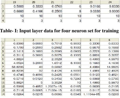
[image:3.595.305.551.50.252.2]ANN modeling has done using feed forward Back propagation algorithm.70% of the available data obtained out of mathematical model is used to train the model and remaining 20% data used for testing and 10% for validation.
[image:3.595.328.514.391.469.2]Table- I: Input layer data for four neuron set for training
Table- II: Input layer data for four neuron set for training
TrainLM is used to train the ANN and Feed Forward Back propagation algorithm is used for supervised learning with bias. Combination of hardlim, purelin, logsig and tansig transfer functions used between input layer to hidden layer and output layer to meet the target. Number of neuron in the hidden layer is arbitrarily used starting from 6 neurons to 28 neurons and the results of the testing data compared with that of analytical values.
Fig.5 Transfer functions used in ANN Model Training of ANN model is done based on the two approches. One approach is to findout the best model basing on the set goal value, and the other approach is for the set goal value the number of epochs the nerwork taking to train the model to achieve the target. I the set target is achievied with small number of epochs the best nerwork modeling is finalised to proceed further for testing and validation. The training curve generated for the ANN model is given in the fig.6 where the goal set is zero error and achieved in the training process is 0.0006
[image:3.595.47.293.588.753.2]Fig.7 Training, validation and testing curve ANN
V. RESULTANDDISCUSSION
Fig.7 shows the trend of training , validation and testing of the single server infinite capacity queueing model using ANN. The simulation process stabilized and reached the target goal of zero error within 11 epoches which indicates the ANN modelled is well weighted with the input and target data sets.
Fig.8 Simulated single server Queuing Model
The probability of number of customers waiting in the queue is simulated and for various intensity values from 0.3 to 0.9 probability of customers waiting is simulated and is shown in the Fig.8. Mathematically calculated values tabulated in Table.III
Fig.8 Error analysis of single server ANN Queuing Model Thus, it is checked that the training procedure was successful. The network converged and produces the correct target outputs for the four input vectors.
The ultimate result of the ANN network is checked for its occuracy by regression analysis against the pridicted output value to the actual inputs given in the input layer values[7]-[10]. MRE, correlation coeffient and RMS values are calculated in evaluating the ANN. Fig.8 shows the error analysis and the R value is alomost equal to 0.999 means the simulated value and target value is almost matching and the error is minimum. Equation number “8” defines the calculation of R value
R(a, p) = cov (a,p)
cov a,a cov (p,p) (8)
Cov(a, p) - covariance between a and p sets that, refer to the actual output and predicted output sets
Cov(a, a) &Cov(p, p) - auto covariance of a and p sets, correspondingly.
The correlation coefficient lies between -1 and +1. R values closer to +1 specify a stronger positive linear relationship while, R values closer to -1 indicate a stronger negative relationship. The mean relative error, which shows the mean ratio between the errors and experimental values, is evaluated by
MRE (%) =𝑁1 𝑁 100 (𝑎𝑖 −𝑝𝑖 )𝑎𝑖
𝑖=1 (9)
Table- III: Results of Mathematical Modeling of a single server queue Traffic
Density
No of customers waiting for service in the queue
0 1 2 3 4 5 6 7 8 9 10
0.3 0.5385 0.3231 0.0969 0.0291 0.0087 0.0026 0.0008 0.0002 0.0001 0 0
0.4 0.434 0.3426 0.1352 0.0534 0.0211 0.0083 0.0033 0.0013 0.0005 0.0002 0.0001
0.5 0.3333 0.3333 0.1667 0.0833 0.0417 0.0208 0.0104 0.0052 0.0026 0.0013 0.0007
0.6 0.25 0.3 0.18 0.108 0.0648 0.0389 0.0233 0.014 0.0084 0.005 0.003
0.7 0.1667 0.2381 0.1701 0.1215 0.0868 0.062 0.0443 0.0316 0.0226 0.0161 0.0115
0.8 0.1176 0.1858 0.1467 0.1158 0.0914 0.0722 0.057 0.045 0.0355 0.028 0.0221
0.9 0.0323 0.0605 0.0567 0.0532 0.0498 0.0467 0.0438 0.0411 0.0385 0.0361 0.0338
VI. CONCLUSION
An Artificial neural network model successfully developed to solve single server infinite capacity queuing problem. The developed model is trained, validated and
with that of analytical model and capable of predicting the target parameters for the given input data with minimum negligible error.
0 0.2 0.4 0.6
0 5 10 15
Pr
o
b
ab
ili
ty o
f c
u
sto
m
e
rs
wai
ting
Number of customers waiting in queue
REFERENCES
1. EBrockmeyer, HLHalstrom, AJensen, “The life and works of AK Erlang”, Trans. Danish Acad. Tech. Sci.(2) (1948).
2. D.G.Kendall, “Some Problems in theory of queues”, Journal of the Royal Statistical Society , vol. 13, 1951, pp. 151-157 and 184-185. 3. J.Abate, W.Whitt, “Transient behavior of the M/M/l queue: Starting at
the origin”, Queueing Systems , vol 2, 1987 pp. 41-65.
4. D.J.Daley, “The Correlation Structure of the Output Process of Some Single Server Queueing Systems”, The Annals of Mathematical Statistics, vol. 3,1968, pp.1007-1019.
5. L.Flatto, “The waiting time distribution for the random order service M/M/1queue”, The Annals of Applied Probability, vol.7, 1997, pp.382-409.
6. G.Koole, A.Mandelbaum,” Queueing Models of Call Centers: An Introduction”, Annals of Operations Research, vol. 113(1-4), 2002, 41-59.
7. R.Kannapiran Palvannan, Kiok Liang Teow, “Queueing for Health care”, Journal of Medical Systems, vol. 36(2), 2012, 541-547. 8. Oblakova, A., Al Hanbali, A., Boucherie, R.J., "An exact root-free
method for the expected queue length for a class of discrete-time queueing systems", Queueing Syst, vol. 92, 2019, pp. 257-292 9. Talak, R., Manjunath, D. & Proutiere, A., "Strategic arrivals to queues
offering priority service", Queueing Syst., 92, 2019, pp. 103-130. 10. M.T.Hagan, H.B.Demuth, M.Beale, “Neural Network Design”, PWS
Publishing Company , Boston,MA,1996.
AUTHORSPROFILE
Sivakami Sundari M, Department Of Bsh, Giet University, Gunupur, India Has 13 Years Of Teaching And Research Experience Has Published Articles In International Journals And Conferences.