SCALABLE HIGH PERFORMANCE MULTIDIMENSIONAL SCALING

(1)

SCALABLE HIGH PERFORMANCE MULTIDIMENSIONAL

SCALING

Seung-Hee Bae

Submitted to the faculty of the University Graduate School

in partial fulfillment of the requirements

for the degree

Doctor of Philosophy

in the Department of Computer Science

Indiana University

(2)

Accepted by the Graduate Faculty, Indiana University, in partial fulfillment of the

require-ments of the degree of Doctor of Philosophy.

Doctoral Committee

Geoffrey C. Fox (Principal Advisor)

Randall Bramley

David B. Leake

January 17, 2012 David J. Wild

(3)

Copyright c

2012

Seung-Hee Bae

(4)

I dedicate this dissertation to my wife (Hee-Jung Kim) and my children (Seewon and Jian).

(5)

Acknowledgements

First of all, I am sincerely grateful to my advisor, Dr. Geoffrey C. Fox, for his insightful guidance and

cheerful encouragement to this dissertation as well as my research projects. On the basis of his guidance and

encouragement, it could be possible to complete Ph.D. degree. While I have been working with him, I could

learn how to research as a scientist.

I would like to thank my research committee members: Dr. Randall Bramley, Dr. David Leake, and Dr.

David Wild for their help, guidance, and invaluable comments to this dissertation. I would like to thank Dr.

Sun Kim, who was my former advisor and had been my research committee member before he left Indiana

University, for his valuable advices and encouragement.

It has been a pleasant time to work with those friendly and brilliant colleagues at Pervasive Technology

Institute (PTI) for five years. I am thankful to Dr. Judy Qiu for her support and discussions for my research.

I am also thankful to SALSA group members: Dr. Jaliya Ekanake, Thilina Gunarathne, Saliya Ekanayake,

Ruan Yang, Hui Li, Tak-Lon Wu, Bingjing Zhang, Yuduo Zhou, Jerome Mitchell, Adam Hughes, and Scott

Beason, for being fantastic lab mates. I am particularly thankful to Dr. Jong Youl Choi for countless valuable

discussions on various research topics as well as non-technical topics during my time at PTI.

I would like to thank administrative staffs of the School of Informatics and Computing and PTI for their

valuable helps to do my study at Indiana University (IU). I am grateful to Ms. Cathy McGregor Foster for

(6)

her helpful advice for Ph.D. study completion, and to Ms. Mary Nell Shiflet and Mr. Gary Miksik for their

administrative support at PTI. Because of their supports, I could focus on my Ph.D. study while I has been at

IU.

Last but not least, I am very much indebted to my family for their generous support and encouragement

throughout my Ph.D. study at IU. My parents and my mother-in-law have been my big supporters during

my Ph.D study, and their encouragement is always cheerful to finish this degree. I cannot fully explain my

gratitude with any words to my lovely wife, Hee-Jung, for her endurance, encouragement, and support with

love for my life as well as my study. Without her support and cheers, I would not make complete this long

journey. Since I met her at Handong, she is the only perfect companion for my life. I would like to thank to

my daughter (Seewon) and son (Jian) for being wonderful children to me. They are the source of my joy and

happiness even though I was in a difficult time.

I am a debtor of love. Thank you, all!

(7)

vii

Seung-Hee Bae

SCALABLE HIGH PERFORMANCE MULTIDIMENSIONAL SCALING

Today is so-called data deluge era. A huge amount of data is flooded in many domains of modern society based on the advancements of technologies and social networks. Dimension reduction is a useful tool for data visualization of such high-dimensional data and abstract data to make data analysis feasible for such large-scale high-dimensional or abstract scientific data. Among the known dimension reduction algorithms, multidimensional scaling (MDS) is investigated in this dissertation due to its theoretical robustness and high applicability. For the purpose of large-scale multidimensional scaling, we need to figure out two main challenges. One problem is that large-scale multidimensional scaling requires huge amounts of computation and memory resources, because it requires O(N2) memory and computation. Another problem is that multidimensional scaling is known as a non-linear optimization problem so that it is easy to be trapped in local optima if EM-like hill-climbing approach is used to solve it.

(8)

List of Tables

3.1 Main matrices used in SMACOF . . . 23

3.2 Cluster systems used for the performance analysis . . . 31

3.3 Runtime Analysis of Parallel Matrix Multiplication part of parallel SMACOF with 50k data

set in Cluster-II . . . 36

4.1 Compute cluster systems used for the performance analysis . . . 59

4.2 Analysis of Maximum Mapping Distance between k-NNs with respect to the number of

near-est neighbors (k). . . . 62

4.3 Large-scale MI-MDS running time (seconds) with 100k sample data . . . 70

(13)

List of Figures

1.1 An example of the data visualization of 30,000 biological sequences by an MDS algorithm,

which is colored by a clustering algorithm. . . 5

3.1 An example of an N_×N matrix decomposition of parallel SMACOF with 6 processes and

2_×3 block decomposition. Dashed line represents where diagonal elements are. . . 25

3.2 Parallel matrix multiplication of N_×N matrix and N_×L matrix based on the decomposition

of Figure 3.1 . . . 27

3.3 Calculation of B(X[k−1])matrix with regard to the decomposition of Figure 3.1. . . 29

3.4 Overall Runtime and partial runtime of parallel SMACOF for 6400 and 12800 PubChem data

with 32 cores in Cluster-I and Cluster-II w.r.t. data decomposition of N_×N matrices. . . . . 40

with 64 cores in Cluster-I and Cluster-II w.r.t. data decomposition of N_×N matrices. . . . . 41

with 128 cores in Cluster-II w.r.t. data decomposition of N_×N matrices. . . . 42

(14)

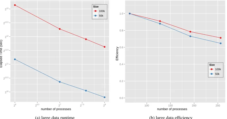
3.7 Performance of parallel SMACOF for 50K and 100K PubChem data in Cluster-II w.r.t. the

number of processes, i.e. 64, 128, 192, and 256 processes (cores). (a) shows runtime and

efficiency is shown at (b). We choose balanced decomposition as much as possible, i.e. 8_×8

for 64 processes. Note that both x and y axes are log-scaled for (a). . . 43

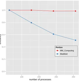
3.8 Efficiency of tMatMult and tMM Computing in Table 3.3 with respect to the number of

processes. . . 44

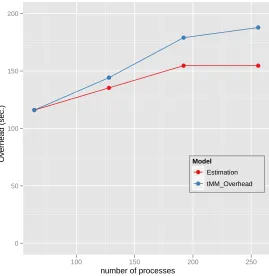
3.9 MPI Overhead of parallel matrix multiplication (tMM Overhead) in Table 3.3 and the rough

Estimation of the MPI overhead with respect to the number of processes. . . 45

3.10 Performance of parallel SMACOF for MC 30000 data in Cluster-I and Cluster-II w.r.t. the

number of processes, i.e. 32, 64, 96, and 128 processes for Cluster-I and Cluster-II, and

extended to 160, 192, 224, and 256 processes for Cluster-II. (a) shows runtime and efficiency

is shown at (b). We choose balanced decomposition as much as possible, i.e. 8_×8 for 64

processes. Note that both x and y axes are log-scaled for (a). . . 46

4.1 Message passing pattern and parallel symmetric pairwise computation for calculating STRESS

value of whole mapping results. . . 56

4.2 Quality comparison between interpolated result of 100k with respect to the number of nearest

neighbors (k) with 50k sample and 50k out-of-sample result. . . . 60

4.3 The illustration of the constrained interpolation space when k=2 or k=3 by initialization at

the center of the mappings of the nearest neighbors. . . 61

4.4 The mapping results of MI-MDS of 100k Pubchem data with 50k sample data and 50k

out-of-sample data with respect to the number of nearest neighbors (k). The sample points are

shown in red and the interpolated points are shown in blue. . . 63

(15)

4.5 Histogram of the original distance and the pre-mapping distance in the target dimension of

50k sampled data of 100k. The maximum original distance of the 50k sampled data is 10.198

and the maximum mapping distance of the 50k sampled data is 12.960. . . 64

4.6 Quality comparison between the interpolated result of 100k with respect to the different

sam-ple sizes (INTP) and the 100k MDS result (MDS) . . . 67

4.7 Running time comparison between the Out-of-Sample approach which combines the full

MDS running time with sample data and the MI-MDS running time with out-of-sample data

when N=100k, with respect to the different sample sizes and the full MDS result of the 100k

data. . . 68

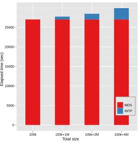
4.8 Elapsed time of parallel MI-MDS running time of 100k data with respect to the sample size

using 16 nodes of the Cluster-II in Table 4.1. Note that the computational time complexity of

MI-MDS isO₍Mn)where n is the sample size and M=N₋n. . . . 69

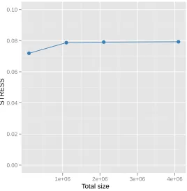
4.9 The STRESS value change of the interpolation larger data, such as 1M, 2M, and 4M data

points, with 100k sample data. The initial STRESS value of MDS result of 100k data is

0.0719. . . 70

4.10 Running time of the Out-of-Sample approach which combines the full MDS running time

with sample data (M=100k) and the MI-MDS running time with different out-of-sample

data sizes, i.e. 1M, 2M, and 4M. . . 71

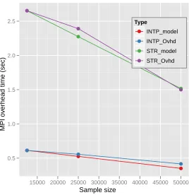
4.11 Parallel overhead modeled as due to MPI communication in terms of sample data size (m)

using Cluster-I in Table 4.1 and message passing overhead model. . . 73

4.12 Parallel overhead modeled as due to MPI communication in terms of sample data size (m)

using Cluster-II in Table 4.1 and message passing overhead model. . . 74

(16)

4.13 Efficiency of the interpolation part (INTP) and the STRESS evaluation part (STR) runtimes

in the parallel MI-MDS application with respect to different sample data sizes using Cluster-I

in Table 4.1. The total data size is 100K. . . 75

4.14 Efficiency of the interpolation part (INTP) and the STRESS evaluation part (STR) runtimes in

the parallel MI-MDS application with respect to different sample data sizes using Cluster-II

in Table 4.1. The total data size is 100K. . . 76

4.15 Interpolated MDS results of total 100k PubChem dataset trained by (a) 12.5k and (b) 50k

sampled data. Sampled data are colored in red and interpolated points are in blue. . . 77

4.16 Interpolated MDS results. Based on 100k samples (a), additional 2M PubChem dataset is

interpolated (b). Sampled data are colored in red and interpolated points are in blue. . . 78

5.1 The computational temperature movement with respect to two different cooling temperature

mechanisms (exponential and linear). . . . 89

5.2 The normalized STRESS comparison of the iris data mapping results in 2D space. The bar

graph illustrates the average of 50 runs with random initialization, and the corresponding error

bar represents the minimum and maximum of the normalized STRESS values of SMACOF,

MDS-DistSmooth with different smoothing steps (s=100 and s=200) (DS-s100 and -s200

hereafter for short), and DA-SMACOF with different cooling parameters (α=0.9, 0.95, and

0.99) (DA-exp90,-exp95, and -exp99 hereafter for short). The x-axis is the threshold value

for the stopping condition of iterations (10−5_{and 10}−6_). _{. . . .} ₉₀

5.3 The 2D median output mappings of iris data with SMACOF (a), DS-s100 (b), and DA-exp95

(c), whose threshold value for the stopping condition is 10−5. Final normalized STRESS

values of (a), (b), and (c) are 0.00264628, 0.00208246, and 0.00114387, correspondingly. . . 92

(17)

5.4 The normalized STRESS comparison of the chemical compound data mapping results in

2D space. The bar graph illustrates the average of 50 runs with random initialization, and the

corresponding error bar represents the minimum and maximum of the normalized STRESS

values of SMACOF, DS-s100 and -s200, and DA-exp90, DA-exp95, and DA-exp99. The

x-axis is the threshold value for the stopping condition of iterations (10−5and 10−6). . . 94

5.5 The normalized STRESS comparison of the breast cancer data mapping results in 2D space.

The bar graph illustrates the average of 50 runs with random initialization, and the

corre-sponding error bar represents the minimum and maximum of the normalized STRESS values

of SMACOF, DS-s100 and -s200, and DA-exp90,DA-exp95, and DA-exp99. The x-axis is

the threshold value for the stopping condition of iterations (10−5and 10−6). . . 96

5.6 The normalized STRESS comparison of the yeast data mapping results in 2D space. The bar

graph illustrates the average of 50 runs with random initialization, and the corresponding error

bar represents the minimum and maximum of the normalized STRESS values of SMACOF,

DS-s100 and -s200, and DA-exp90,DA-exp95, and DA-exp99. The x-axis is the threshold

value for the stopping condition of iterations (10−5and 10−6). . . 97

5.7 The average running time comparison between SMACOF, MDS-DistSmooth (s=100), and

DA-SMACOF (DA-exp95) for 2D mappings with tested data sets. The error bar

repre-sents the minimum and maximum running time. EM-5/EM-6 reprerepre-sents SMACOF with

10−5/10−6threshold, and DS-5/DS-6 and DA-5/DA-6 represents the runtime results of

MDS-DistSmooth and DA-SMACOF, correspondingly, in the same way. . . 98

(18)

5.8 The normalized STRESS comparison of the metagenomics sequence data mapping results in

2D and 3D space. The bar graph illustrates the average of 10 runs with random initialization,

and the corresponding error bar represents the minimum and maximum of the normalized

STRESS values of SMACOF and DA-SMACOF withα=0.95. The x-axis is the threshold

value for the iteration stopping condition of the SMACOF and DA-SMACOF algorithms

(10−5and 10−6). . . 101

5.9 The normalized STRESS comparison of the ALU sequence data mapping results in 2D and

3D space. The bar graph illustrates the average of 10 runs with random initialization, and the

corresponding error bar represents the minimum and maximum of the normalized STRESS

values of SMACOF and DA-SMACOF withα=0.95. The x-axis is the threshold value for

the iteration stopping condition of the SMACOF and DA-SMACOF algorithms (10−5and

10−6). . . 102

5.10 The normalized STRESS comparison of the 16s RNA sequence data with 50000 sequences

for mapping in 2D and 3D space. The bar graph illustrates the average of 10 runs with random

initialization, and the corresponding error bar represents the minimum and maximum of the

normalized STRESS values of SMACOF, DA-SMACOF withα =0.95 (DA-exp95), and

DA-SMACOF with linear cooling with 100 steps (DA-lin100). The x-axis is the threshold

(10−5, 10−6, and hybrid approach). . . 104

5.11 The mapping progress of DA-SMACOF with RNA50k data set in 2D space with respect to

computational temperature (T ) and corresponding normalized STRESS value (σ). . . 107

(19)

5.12 The normalized STRESS comparison of the 16s RNA sequence data with 100000 sequences

for mapping in 2D and 3D space. The bar graph illustrates the average of 10 runs with random

initialization, and the corresponding error bar represents the minimum and maximum of the

normalized STRESS values of SMACOF, DA-SMACOF withα =0.95 (DA-exp95), and

DA-SMACOF with linear cooling with 100 steps (DA-lin100). The x-axis is the threshold

(10−5, 10−6, and hybrid approach). . . 108

5.13 The normalized STRESS progress comparison of MC 30k data in 2D and 3D space by

SMA-COF and exp95. The x-axis is the cummulated iteration number of SMASMA-COF and

DA-SMACOF algorithms. . . 110

5.14 The normalized STRESS progress comparison of RNA50k data in 2D and 3D space by

SMA-COF and exp95. The x-axis is the cummulated iteration number of SMASMA-COF and

DA-SMACOF algorithms. . . 112

5.15 The average running time comparison between SMACOF and DA-SMACOF (DA-exp95) for

2D and 3D mappings with MC30000 and ALU50058 data sets. The error bar represents the

minimum and maximum running time. EM-5/EM-6 represents SMACOF with 10−5/10−6

threshold, and DA-5/DA-6 represents the runtime results of DA-SMACOF, correspondingly,

in the same way. . . 113

5.16 The average running time comparison between SMACOF, DA-SMACOF (DA-exp95), and

DA-SMACOF with linear cooling (DA-lin100) for 2D and 3D mappings with 16s RNA

data sets. The error bar represents the minimum and maximum running time. EM-5/EM-6

represents SMACOF with 10−5/10−6threshold, and DA-e5/DA-e5,6/DA-6 and

DA-l5/DA-l5,6/DA-l6 represents the runtime results of DA-exp95 and DA-lin100, correspondingly, with

10−5_/hybrid(10−5_{and 10}−6_)/10−6_{. . . 115}

(20)

1 Introduction

1.1 Introduction

Because of the advancements of technology, a huge amount of data are produced in many domains of

modern society, from digital personal information to scientific observation, and experimental data to medical

records data. The current era could be referred to as the so-called data deluge era. In many scientific domains,

the volumes of data are on the tera-scale and even the peta-scale. For the study of large-scale sky surveys

in astronomy, about 20 terabytes of sky image data are collected by the Large Synoptic Survey Telescope1

per night, and this phenomenon has led to about 60 petabytes of raw data over ten years of operations. In

addition to large-scale sky survey data, biological sequence data has been produced in unimaginable volumes.

Although the Human Genome Project2, which was finished in 2003, was completed in 13 years and cost

billions of dollars, now genome sequencing for an organism can be done much faster and more cheaply due

to cost-effective high-throughput sequencing technologies. In fact, innovative sequencing technologies and

the microarray technique have increased the volumes of biological data enormously.

1_{LSST: Large Synoptic Survey Telescope (http://www.lsst.org/lsst/)}

2_{Human Genome Project (http://www.ornl.gov/sci/techresources/Human Genome/home.shtml)}

(21)

1. Introduction 2

In 2005, Intel proposed the Recognition, Mining, and Synthesis (RMS) [24] approach as a killer

ap-plication for the next data explosion era. Machine learning and data mining algorithms were suggested as

important algorithms for the data deluge era by [24]. Mining some meaningful information from these large

volumes of raw data requires a huge amount of computing power which exceeds a single computing machine.

To make matters worse, the asymptotic time complexities of most of the data mining algorithms are larger

than a simpleO₍_N₎_{, in that they require a significant amount of processing capability for analyses over large}

volumes of data. Thus, parallel and distributed computing is a critical feature of performing such data

analy-ses. The efficiency and the scalability should be achieved in a parallel implementation of algorithms in order

to maximize the effects of parallel and distributed computing.

One of the innovative inventions that has emerged in the computer hardware community during the last

decade was the invention of multi-core architecture. The classical method of improving the computing power

of computing processing units (CPUs), such as increasing clock speed, has been limited by physical obstacles;

therefore, the CPU companies changed the focus of improving computing power from increasing the clock

speed of a CPU to increasing the number of cores in a CPU chip. Since multicore architecture as invented,

multicore architecture has become important in software development with effects on the client, the server

and supercomputing systems [5, 23, 24, 66]. As mentioned in [66], the parallelism has become a critical issue

for developing software for the purpose of effectively using multicore systems.

From the above statements, the necessary computation will be enormous for data mining algorithms in the

future, and classical sequential programming schemes will not be suitable for multicore systems any more,

so that implementing in scalable parallelism these algorithms will be one of the most important procedures

for the coming many-core and data explosion era.

Among the many data mining areas which exist, such as clustering, classification, and association rule

mining, and so on, dimension reduction algorithms are used to visualize high-dimensional data or abstract

(22)

1. Introduction 3

which can be applied to usage to fulfill the following purposes: (1) representing unknown data distribution

structures in human-perceptible space with respect to the pairwise proximity or topology of the given data;

(2) verifying a certain hypothesis or conclusion related to the given data by showing the distribution of the

data; and (3) investigating relationship among the given data by spatial display.

Among the known dimension reduction algorithms, such as Principal Component Analysis (PCA),

Multi-dimensional Scaling (MDS) [13, 45], Generative Topographic Mapping (GTM) [11, 12], and Self-Organizing

Maps (SOM) [43], to name a few, multidimensional scaling (MDS) has been extensively studied and used

in various real application areas, such as biology [48, 71], stock market analysis [33], computational

chem-istry [4], and breast cancer diagnosis [46]. This dissertation focuses on the MDS algorithm, and we investigate

two ultimate goals: (1) how to achieve the scalability of the MDS algorithm to deal with large-scale data; and

(2) how to improve the mapping quality of MDS solutions as well as the scalable MDS. This dissertation also

describes some detailed performance analyses and experiments related to the proposed methodologies.

1.2 Multidimensional Scaling (MDS)

Multidimensional scaling (MDS) [13, 45, 68] is a general term that refers to techniques for constructing a

map of generally high-dimensional data into a target dimension (typically a low dimension) with respect to

the given pairwise proximity information. Mostly, MDS is used to visualize given high dimensional data or

abstract data by generating a configuration of the given data which utilizes Euclidean low-dimensional space,

i.e. two-dimension or three-dimension.

Generally, proximity information, which is represented as an N_×N dissimilarity matrix (∆= [δi j]),

where N is the number of points (objects) andδi jis the dissimilarity between point i and j, is given for the

(23)

1. Introduction 4

technique is to construct a configuration of a given high-dimensional data into low-dimensional Euclidean

space, where each distance between a pair of points in the configuration is approximated to the

correspond-ing dissimilarity value as much as possible. The output of MDS algorithms could be represented as an N_×L

configuration matrix X, whose rows represent each data point xi (i=1, . . . ,N) in L-dimensional space. It is

quite straightforward to compute the Euclidean distance between xiand xjin the configuration matrix X , i.e.

di j(X) =kxi−xjk, and we are able to evaluate how well the given points are configured in the L-dimensional

space by using the suggested objective functions of MDS, called STRESS [44] or SSTRESS [67]. Definitions

of STRESS (1.1) and SSTRESS (1.2) are following:

σ(X) =

∑

i<j≤N

wi j(di j(X)−δi j)2 (1.1)

σ2₍_X₎ ₌

∑

i<j≤N

wi j[(di j(X))2−(δi j)2]2 (1.2)

where 1_≤i< j_≤N and wi jis a weight value, so wi j≥0.

As shown in the STRESS and SSTRESS functions, the MDS problems could be considered to be

non-linear optimization problems, which minimizes the STRESS or the SSTRESS function in the process of

configuring an L-dimensional mapping of the high-dimensional data.

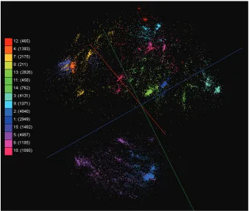
Figure 1.1 is an example of the data visualization of 30,000 biological sequence data, which is related to

a metagenomics study, by an MDS algorithm. The colors of the points in Figure 1.1 represent the clusters

of the data, which is generated by a pairwise clustering algorithm by deterministic annealing [36]. The data

visualization in Figure 1.1 shows the value of the dimension reduction algorithms which produced lower

dimensional mapping for the given data. We can see clearly the clusters without quantifying the quality of

(24)

[image:24.612.143.505.121.428.2]

1. Introduction 5

Figure 1.1: An example of the data visualization of 30,000 biological sequences by an MDS algorithm, which is colored by a clustering algorithm.

1.3 Motivation

The recent explosion of publicly available biological gene sequences, chemical compounds, and various

scientific data offers an unprecedented opportunity for data mining. Among the various available data mining

algorithms, dimension reduction is a useful tool for information visualization of high-dimensional data to

make analysis feasible for large volume and high-dimensional scientific data. It facilitates the investigation

of unknown structures of high dimensional data in three (or two) dimensional visualization.

In contrast to other algorithms, like PCA, GTM, and SOM, which generally construct a low dimensional

(25)

1. Introduction 6

dimension on the basis of pairwise proximity (typically dissimilarity or distance) information; as a result, it

does not require feature vector information of the underlying application data to acquire a lower dimensional

mapping of the given data. Hence, MDS is an extremely useful approach for data visualization of a certain

type of data, which would prove impossible or improper to represent by feature vectors but tat has pairwise

dissimilarity, such as a biological sequence data. MDS, of course, is also applicable to data represented by

feature vectors as well. MDS provides more broad applicability than other dimension reduction methods in

terms of the given format of the data.

In the past, the data size given dealt with by machine learning and data mining algorithms was usually

small enough to be executed on a single CPU or node without any consideration of parallel computing. On the

other hand, in the modern data-deluged world, we can find many interesting data sets with large amounts of

units which are impossible to run as sequential programming on a single node due, not only to the prohibitive

computing requirements but also, because of the required memory size. Therefore, we have to figure out

how to increase the computational capability of the MDS algorithm in order to manage large-scale

high-dimensional data sets. In addition to the increase of data size, the invention and emergence of multi-core

architectures has also required a change in the programming paradigm, so as to be able to utilize the maximal

performance of the multi-core chips.

In general, there are two different approaches with which to improve the computing capability of MDS

algorithm. One is to increase the available computing resources, i.e. CPUs and main memory size, and the

other method is to reduce the computational time complexity.

In addition to the motivation of increasing computational capability because of the large scale of the

data, another motivation of this thesis is based on the fact that the MDS problem is a non-linear optimization

problem, which means it might have many local optima, so the avoidance of non-global local optima is an

essential property needed in order to obtain a better quality of MDS outputs. Also, if we achieve the local

(26)

1. Introduction 7

output, than the output of the MDS algorithm which suffers from being trap in local optima. Thus, this

dissertation also investigates how to avoid local optima effectively and efficiently.

1.4 The Research Problem

The explosion of data and the invention of multi-core architecture has brought forth interesting reseach

issues in the data mining community as well as other computer science areas. We reviewed the interesting

research motivations in relation to the MDS algorithm in Section 1.3. As we discussed in Section 1.3, two

main goals of this dissertation are: (1) examining the scalability of the MDS algorithm due to the large-scale

of the given data, i.e. millions of points; and (2) the local optima avoidance issue of MDS, which is a

non-linear optimization problem. These motivations of this dissertation have lead us to the following research

problems:

Parallelization

Applying distributed parallelism to the MDS algorithm is a natural process for achieving an increase in

the computational capability by using distributed computing nodes. This makes it possible to acquire

more computing resources and to utilize the full power of multi-core systems. Several issues should

be covered to implement an algorithm in parallel, such as the load-balance, efficiency, and scalability

issues.

Reduction of Complexity

Since the time complexity and memory requirements of the MDS algorithm is O₍_N2₎_{due to the use}

of an N by N pairwise dissimilarity matrix, where N is the number of points, and the distributed

paral-lel implementation of MDS algorithm is still limited to the number of available computing resources,

(27)

1. Introduction 8

requirement, is required to reach the goal of scalability of the MDS algorithm. The parallel

implemen-tation of the proposed MDS approach will be highly encouraged because the size of the data could be

enormous.

Optimization Method

Trapping in a local optima problem is a well-known problem of the non-linear optimization methods,

including MDS problem. This is a very important issue for the non-linear optimization problems to

avoid local optima. However, it is difficult to avoid local optima by using simple heuristics, which

are based on the hill-climbing optimization method. Various non-determinstic optimization methods,

such as the Genetic Algorithms (GA) [37] and Simulated Annealing (SA) [40], were proposed as

solutions of local optima avoidance problems. They have been used for many non-linear optimization

problems. As with other data mining algorithms, various optimization methods have been applied to

the MDS problem for the purpose of avoiding local optima. It is true that the GA and SA algorithms

are very successful for avoiding local optima, which is the goal of these algorithms. These algorithms,

however, are also known to suffer from long running times due to their non-deterministic random

walking approach. By taking the above statements into consideration, we would like to solve the local

optima issue of the MDS problem by applying a deterministic optimization method, which is not based

on a simple gradient descent approach.

1.5 Contributions

We can summarize the contributions of this dissertation as being the purpose of improving MDS

algo-rithms in relation to computational capability and mapping quality such as the following:

• [Parallelization] Efficient parallel implementation via the Message Passing Interface (MPI) in order to

(28)

1. Introduction 9

systems, i.e. cluster systems.

• [Reducing Complexity] Development of an innovative algorithm, which reduces the computational

complexity and memory requirement of MDS algorithms, and which produces acceptable mapping

results; this step will be taken for the purpose of scaling the MDS algorithm’s capacity up to millions

of points, a step which is usually intractable for generating a mapping via normal MDS algorithms.

• [Local Optima Avoidance] Providing an MDS algorithm which could comprehend out the local

op-tima avoidance problem in a deterministic way so that it generates better quality mapping in a

reason-able amount of time.

1.6 Dissertation Organization

This dissertation is composed of several chapters and each chapter describes a unique part of this thesis

as follows:

In Chapter 2, we describe some background methodologies related to this dissertation. First, we discussed

the well-known MDS algorithm which is named Scaling by a MAjorizing of a COmplicated Function

(SMA-COF). This is implemented in distributed parallel fashion in Chapter 3. Also, we summarize the optimization

method, named Deterministic Annealing (DA), which aims at avoiding local optima and which is used in this

dissertation. The Message Passing Interface (MPI) standard is briefly mentioned in this chapter as well.

How to achieve distributed parallel implementation of the SMACOF algorithm is illustrated in detail

in Chapter 3. Since the load balance has a critical impact on the efficiency of the parallel implementations, we

discuss how to decompose and spread out the given data to each process; this approach is directly connected

to the load balance issue. Furthermore, we described the message passing patterns of each components of

(29)

1. Introduction 10

on the testing results on two different cluster systems, follows the explanation of the parallel implementation

in Chapter 3.

Chapter 4 describes the interpolation algorithm of the MDS problem which reduces computational

com-plexity fromO₍_N2₎_to_O₍_nM₎_{, where N is the full data size, n is the sampled data size, and M}₌_N₋_n.

Furthermore, we introduce how to parallelize the proposed interpolation algorithm of MDS due to the huge

amounts of data points. This section is followed by a discussion of a quality comparison between the

pro-posed interpolation algorithm and the full MDS algorithm, as well as parallel performance analysis of the

parallelized implementation of this algorithm.

In contrast to Chapter 3 and Chapter 4, which focus on scaling up the computing capability of MDS

algorithms, we propose the step of applying the deterministic annealing (DA) [62, 63] optimization method

to the MDS problem; this approach will result in an avoidance of local optima in a deterministic way. This

information is presented in Chapter 5. In Chapter 5, we also compare the DA applied MDS algorithm with

other MDS algorithms, with respect to the mapping quality and running time.

Finally, in Chapter 6, we present the conclusions of this dissertation and future research interests related

(30)

2 Backgrounds

2.1 Classical Multidimensional Scaling

The classical scaling (Classical MDS) was the first practical technique available for MDS, which was

proposed by Torgerson [68, 69] and Gower [31]. The linear algebraic theorems mentioned by Eckart and

Young [25] and Young and Householder [75] are the bases of the classical MDS. The main idea of the classical

MDS is that, if the dissimilarities are represented by Euclidean distances, then we can find the configurations

which represent the dissimilarities by using some matrix operations. Here, we briefly introduce the classical

MDS algorithm, and the algorithm is explained in detail in Chapter 12 of [13].

The matrix of squared Euclidean distances of the given coordinates (D(2)(X)or simply D(2)) can be

expressed by a simple matrix equation with respect to the coordinate matrix (X), as shown in (2.1) and (2.2):

D(2) = c1t+1ct₋2XXt (2.1)

= c1t+1ct₋2B, (2.2)

(31)

2. Backgrounds 12

where c is the diagonal elements of XXt, 1 is the one vector whose elements are all ONE, 1t, ct, and Xt

are transpose of 1, c, and X, correspondingly, and B=XXt. (2.1) illustrates the relation between the squared

distances and the scalar products of the coordinate matrix (X).

The centering matrix (J) can be defined as J=I₋n−111t, where I is the identity matrix, which translates

a matrix to a column centered matrix by multiplying them. By multiplying the left and the right sides by the

centering matrix J, a process called the double centering operation, we can introduce the following equations:

JD(2)J = J(c1t+1ct₋2XXt)J (2.3)

= Jc1tJ+J1ctJ₋J(2B)J (2.4)

= Jc0t+0ctJ₋2JBJ (2.5)

= −2JBJ (2.6)

= −2B. (2.7)

Since the centering of a vector of ones turns out to be a vector of zeros (1tJ=J1=0), the first two

terms are elliminated. Without a loss of generality, we can assume that the coordinate matrix (X) is a column

centered matrix. Then, the result of the double centering operation on the B matrix is equal to B itself, since

X is a column centered matrix. Therefore, we can define the relation between B and D(2)as in (2.8).

B=−1₂JD(2)J. (2.8)

(32)

2. Backgrounds 13

Algorithm 2.1 Classical MDS algorithm

1: Calculate the matrix of squared dissimilarity∆(2).

2: Compute B∆by applying double centering: B∆=−1 2J∆

(2)_J.

3: Compute the eigendecomposition of B∆=QΛQt.

4: /* Q₊is the first L eigenvectors of Q */

5: /*Λ+is the first L eigenvalues ofΛwhich is greater than ZERO. */ 6: Calculate L-dimensional coordinate matrix X by X=Q₊Λ1₊/2.

7: return X.

B = QΛQt (2.9)

= QΛ1/2Λ1/2Qt (2.10)

= QΛ1/2(Λ1/2)tQt (2.11)

= (QΛ1/2)(QΛ1/2)t₌_XXt_. _(2.12)

By (2.12), we can find the coordinate matrix from the given squared distance matrix. The classical MDS

is very close to the above method, and the only difference is that it uses the squared dissimilarity matrix (∆(2)) instead of the matrix of squared distances (D(2)).

Algorithm 2.1 describes the classical MDS procedure, and its computational time complexity isO₍N3₎

due to the eigendecomposition. Note that, if∆is not a Euclidean distance matrix, some eigenvalues could be negative. The classical MDS algorithm ignores those negative eigenvalues as errors. Since the classical MDS

is an analytical solution, it does not require iterations to get a solution as shown in Algorithm 2.1. Another

merit of the classical MDS is that it provides nested solutions, in that the two dimensions of a 2D solution

are the same as the first two dimensions of a 3D result. The objective function of the classical MDS is called

(33)

2. Backgrounds 14

Algorithm 2.2 SMACOF algorithm

1: Z_⇐X[0];

2: k_⇐0;

3: ε⇐small positive number;

4: MAX_⇐maximum iteration;

5: Computeσ[0]=σ(X[0]);

6: while k=0 or (∆σ>εand k_≤MAX ) do

7: k_⇐k+1;

8: X[k]=V†B(X[k−1])X[k−1]

9: Computeσ[k]=σ(X[k])

10: Z_⇐X[k];

11: end while

12: return Z;

S(X) =||XXt₋B∆||2. (2.13)

2.2 Scaling by a MAjorizing of a COmplicated Function (SMACOF)

There are a lot of different algorithms which could be used to solve the MDS problem, and Scaling by

MAjorizing a COmplicated Function (SMACOF) [20, 21] is one of them. SMACOF is an iterative

majoriza-tion algorithm used to solve the MDS problem with the STRESS criterion. The iterative majorizamajoriza-tion

proce-dure of the SMACOF could be thought of as an Expectation-Maximization (EM) [22] approach. Although

SMACOF has a tendency to find local minima due to its hill-climbing attribute, it is still a powerful method

since the algorithm, theoretically, guarantees a decrease in the STRESS (σ) criterion monotonically. Instead

of a mathematically detail explanation of the SMACOF algorithm, we illustrate the SMACOF procedure in

this section. For the mathematical details of the SMACOF algorithm, please refer to [13].

Algorithm 2.2 illustrates the SMACOF algorithm for the MDS solution. The main procedure of the

SMACOF are its iterative matrix multiplications, called the Guttman transform, as shown in Line 8 in

Al-gorithm 2.2, where V†is the Moore-Penrose inverse [52, 54] (or pseudo-inverse) of matrix V . The N_×N

(34)

2. Backgrounds 15

V = [vi j] (2.14)

vi j =       

−wi j if i6=j

∑i₆=jwi j if i=j

(2.15)

B(Z) = [bi j] (2.16)

bi j =                 

−wi jδi j/di j(Z) if i6=j

0 if di j(Z) =0,i6=j

−∑i6=jbi j if i=j

(2.17)

If the weights are equal to one (wi j=1) for all pairwise dissimilarities, then V and V† are simplified as

follows:

V = N

I₋ee

t

N

(2.18)

V† = 1

N

I₋ee

t

N

(2.19)

where e= (1, . . . ,1)t_{is one vector whose length is N. In this thesis, we generate mappings based on the equal}

weights weighting scheme and we use (2.19) for V†.

As in Algorithm 2.2, the computational complexity of the SMACOF algorithm is O₍_N2₎_{, since the}

Guttman transform performs a multiplication of an N_×N matrix and an N_×L matrix twice, typically N_≫L

(L=2 or 3), and the computation of the STRESS value, B(X[k]), and D(X[k])also takeO₍_N2₎_{. In addition,}

the SMACOF algorithm requiresO₍_N2₎_{memory because it needs several N}_×_{N matrices, as in Table 3.1.}

Due to the trends of digitization, data sizes have increased enormously, so it is critical that we are able to

(35)

2. Backgrounds 16

single node computer due to the memory requirement increases inO₍_N2₎_{. In order to remedy the shortage}

of memory in a single node, we illustrate how to parallelize the SMACOF algorithm via message passing

interface (MPI) for utilizing distributed-memory cluster systems in Chapter 3.

2.3 Message Passing Interface (MPI)

The Message Passing Interface (MPI) [27,73] standard is a language-independent message passing

proto-col, and is the one of the most widely used parallel programming methods in the history of parallel computing.

MPI is a library specification for a message passing system, which aims at utilizing distributed computing

resources, i.e. computer cluster systems, for the purpose of increasing the computing power to deal with the

large scale problem caused by the communication between processes via messages.

MPI specification is composed of the definitions of a set of routines used to illustrate various

paral-lel programming models effectively, such as point-to-point communication, collective communication, the

topologies of communicators, derived data types, and parallel-IO. Since MPI uses language-independent

specifications for calls and language bindings, MPI runtimes are available for many programming languages,

for instance, Fortran, C, C++, Java, C#, Python, and so on.

MPI communication procedures can be categorized by two different mechanisms: (i) a point-to-point

communication procedure in which a communication is operated between two processes; and (ii) a collective

communication procedure, in which all processes within a communication group should invoke the collective

communication procedure.

A point-to-point communication can occur with a pair of send and receive operations. The MPI send

and receive operations are divided into: (i) a blocking operation and (ii) a nonblocking operation. In [27],

(36)

2. Backgrounds 17

blocking If a return from the procedure indicates the user is allowed to re-use resources specified in the call.

nonblocking If the procedure may return before the operation completes, and before the user is allowed to

re-use resources (such as buffers) specified in the call.

In addition to a standard mode, MPI also proposes three more communication modes: the (i) buffered,

(ii) synchronous, and (iii) ready modes. In the standard communication mode, MPI decides whether the

outgoing message will be buffered or not, not by users, so that a stardard mode send operation can be started

regardless of posting of the matching receive; this command may be complete before a maching receive is

posted, or it will not complete until a maching receive has been posted and the data has been moved to the

receiver. A buffered mode send operation is defined as a local procedure so that it depends only on the local

process and can complete without regard to other processes. In fact, MPI must buffer the outgoing message

of a buffered mode send operation so it can complete in the local region. In the synchronous communication

mode, a send operation can be started regardless of posting of the matching receive, similar to the standard

and buffered modes. However, it will not complete successfully until a matching receive operation is posted

and the receive operation has started to receive the message of the synchronous send. A send in the ready

mode may be started only if the matching receive operation is already posted, unlike a send operation in

other communication modes. Both blocking and nonblocking send operations can use these four different

communication modes explained above.

Several collective communication procedures are defined in the MPI standard [27]: barrier

synchroniza-tion, broadcast, scatter, gather, allgather, scatter/gather (which is complete exchange or all-to-all), and

reduc-tion/allreduction operations i.e. sum, min, max, or user defined functions. A collective operation requires

that all processes in the communication group call the communication routine.

MPI is highly used under distributed cluster systems, which connected via a high-speed network; it is

(37)

2. Backgrounds 18

large-scale data-intensive or computing-intensive applications. MPI also supports various communication

topologies, such as 2D or 3D grids and general graphs topologies, as well as dynamic communiation groups.

In addition, new types of functionality, such as dynamic processes, one-sided communication, parallel I/O,

and so on, are added to MPI standard 2 [26]. MPI provides flexible fine-grained parallel programming

environment based on various features of MPI.

2.4 Threading

Emerging multicore processors places a spotlight parallel computing, including threading, since it is able

to supply many computing units in a single node and even in a single CPU. Threading is used to investigate

parallelism within shared memory systems, such as graphics processors, multicore systems, and Symmetric

Multiprocessor (SMP) Systems.

Threading supports fine grained task parallelism, which could be effective for various applications

with-out message passing overhead. For the correct use of threading, however, we have to consider the following:

(i) dealing with critical sections, which should be mutually exclusive between threads; and (ii) cache false

sharing overhead and cache line effects. There are a lot of threading libraries, which suppport parallelism

via threads, such as POSIX Threads [15], OpenMP [3], the Task Parallel Library (TPL) [47], Intel Threading

Building Blocks (TBB) [2, 60], and the Boost library [1, 39], to name a few. The Concurrency and

Coordi-nation Runtime (CCR) [18, 61] library supports a more complicated threading parallelism through message

passing via Port, which can be thought of as a way to queue messages. In addition to these libraries, most

programming languages also support threading in various forms.

Since multicore technology has been invented, multicore CPUs have become universal and typical, in that

most cluster systems are multicore cluster systems. Multicore cluster systems are distributed memory systems

(38)

2. Backgrounds 19

programming paradigms, which combine distributed memory parallelism via MPI for inter-node

communi-cations and shared memory parallelism via threading libraries, i.e. OpenMP and TPL, within each node, have

been investigated [56, 59]. In this dissertation, I have used the hybrid parallel paradigm in Chapter 4 as well.

2.5 Deterministic Annealing (DA)

Since the simulated annealing (SA) was introduced by Kirkpatrick et al. [40], people widely accepted

SA and other stochastic maximum entropy approaches to solve optimization problems for the purpose of

finding global optimum instead of hill-climbing deterministic approaches. SA is a Metropolis algorithm [51],

which accepts not only the better proposed solution but even the worse proposed solution than the previous

solution, based on a certain probability which is related to the computational temperature (T ). Also, it is

known that the Metropolis algorithm converges to an equilibrium probability distribution known as the Gibbs

probability distribution. If we denoteH₍_X₎_{as the energy (or cost) function and}F _{as a free energy, then}

Gibbs distribution density as follows:

PG(X) =exp

−_T1(H₍_X₎₋F₎

, (2.20)

F ₌₋_{T log} Z

exp

−_T1H₍_X₎

dX. (2.21)

and the free energy (F_{), which is a suggested objective function of SA, is minimized by the Gibbs probability}

density PG. Also, free energyF _{can be written as follows:}

F_P₌_<H _>_P₋TS₍P) (2.22)

≡ Z

P(X)H₍_X₎_dX₊_T Z

(39)

2. Backgrounds 20

where<H>Prepresents the expected energy and S(P)denotes entropy of the system with probability

density P. Here, T is used as a Lagrange multiplier to control the expected energy. With a high temperature,

the problem space is dominated by the entropy term which makes the problem space become smooth so

it is easy to move further. As the temperature is getting cooler, however, the problem space is gradually

revealed as the landscape of the original cost function which limits the movement within the problem space.

To avoid being trapped in local optima, people usually start with a high temperature and slowly decrease the

temperature in the process of finding a solution.

SA relies on random sampling with the Monte Carlo method to estimate the expected solution, e.g.

ex-pected mapping in target dimension for MDS problem, so that it suffers from a long running time.

Deter-ministic annealing (DA) [62, 63] can be thought of as an approximation algorithm of SA which tries to keep

the merits of SA. The DA [62, 63] method actually tries to calculate the expected solution exactly or

approx-imately with respect to the Gibbs distribution as an amendment of SA’s long running time, while it follows

(40)

3 High Performance Multidimensional Scaling

3.1 Overview

Due to the innovative advancements in science and technology, the amount of data to be processed or

analyzed is rapidly growing and it is already beyond the capacity of most commodity hardware we are using

currently. To keep up with such fast development, study for data-intensive scientific data analyses [28] has

been already emerging in recent years. It is a challenge for various computing research communities, such as

high-performance computing, database, and machine learning and data mining communities, to learn how to

deal with such large and high dimensional data in this data deluged era. Unless developed and implemented

carefully to overcome such limits, techniques will face soon the limits of usability. Parallelism is not an

optional technology any more but an essential factor for various data mining algorithms, including dimension

reduction algorithms, by the result of the enormous size of the data to be dealt by those algorithms (especially

since the data size keeps increasing).

Visualization of high-dimensional data in low-dimensions is an essential tool for exploratory data

anal-ysis, when people try to discover meaningful information which is concealed by the inherent complexity of

the data, a characteristic which is mainly dependent on the high dimensionality of the data. This task is also

(41)

3. High Performance Multidimensional Scaling 22

getting more difficult and challenged by the huge amount of the given data. In most data analysis with such

large and high-dimensional dataset, we have observed that such a task is no more CPU bounded but rather

memory bounded, in that any single process or machine cannot hold the whole data in its memory any longer.

In this chapter, I tackle this problem for developing a high performance visualization for large and

high-dimensional data analysis by using distributed resources with parallel computation. For this purpose, we will

show how we developed a well-known dimension-reduction-based visualization algorithm, named

Multidi-mensional Scaling (MDS), in the distributed fashion so that one can utilize distributed memories and be able

to process large and high dimensional datasets.

In this chapter, we introduce the details of our parallelized version of an MDS algorithm, called parallel

SMACOF, in Section 3.2. The brief introduction of SMACOF [20, 21] can be found at Section 2.2 of

Chap-ter 2. In the next, we show our performance results of our parallel version of MDS in various compute clusChap-ter

settings, and we present the results of processing up to 100,000 data points in Section 3.3 followed by the

summary of this chapter in Section 3.4.

3.2 High Performance Visualization

We have observed that processing a very large dataset is not only a cpu-bounded but also a

memory-bounded computation, in that memory consumption is beyond the ability of a single process or even a single

machine, and that it will take an unacceptable running time to run a large data set even if the required

memory is available in a single machine. Thus, running machine learning algorithms to process a large

dataset, including MDS discussed in this thesis, in a distributed fashion is crucial so that we can utilize

multiple processes and distributed resources to handle very large data which usually will take a long time and

even not fit in the memory of a single process or a compute node. The memory shortage problem becomes

(42)

Table 3.1: Main matrices used in SMACOF Matrix Size Description

∆ N_×N Matrix for the given pairwise dissimilarity[δi j]

D(X) N_×N Matrix for the pairwise Euclidean distance of mapped in target dimension[di j]

V N_×N Matrix defined by the value vi jin (2.14)

V† N_×N Matrix for pseudo-inverse of V

B(Z) N_×N Matrix defined by the value bi jin (2.16)

W N_×N Matrix for the weight of the dissimilarity[wi j]

X[k] N_×L Matrix for current L-dimensional configuration of N data points x[_ik](i=1, . . . ,N)

X[k−1] N_×L Matrix for previous L-dimensional configuration of N data points x[_ik−1](i=1, . . . ,N)

process large data with efficiency, we have developed the parallel version of MDS by using a Message Passing

Interface (MPI) fashion. In the following, we will discuss more details on how we decompose data using the

MDS algorithm to fit in the memory limit of a single process or machine. We will also discuss how to

implement an MDS algorithm, called SMACOF, by using MPI primitives to get some computational benefits

of parallel computing.

3.2.1 Parallel SMACOF

Table 3.1 describes frequently used matrices in the SMACOF algorithm. As shown in Table 3.1, the

memory requirement of SMACOF algorithm increases quadratically as N increases. For the small dataset,

memory would not be any problem. However, it turns out to be a critical problem when we deal with a large

data set, such as hundreds of thousands or even millions. For instance, if N=10,000, then one N_×N matrix

of 8-byte double-precision numbers consumes 800 MB of main memory, and if N=100,000, then one N×N

matrix uses 80 GB of main memory. To make matters worse, the SMACOF algorithm generally needs six

N_×N matrices as described in Table 3.1, so at least 480 GB of memory is required to run SMACOF with

(43)

temporary buffers.

If the weight is uniform (wi j=1,∀i,j), we can use only four constants for representing N×N V and V†

matrices in order to saving memory space. We, however, still need at least three N_×N matrices, i.e. D(X),∆, and B(X), which requires 240 GB memory for the above case, which is still an unfeasible amount of memory

for a typical computer. That is why we have to implement a parallel version of SMACOF with MPI.

To parallelize SMACOF, it is essential to ensure load balanced data decomposition as much as possible.

Load balance is important not only for memory distribution but also for computational distribution, since

parallelization implicitly benefits computation as well as memory distribution, due to less computing per

process. One simple approach of data decomposition is that we assume p=n2, where p is the number of

processes and n is an integer. Though it is a relatively less complicated decomposition than others, one major

problem of this approach is that it is a quite strict constraint to utilize available computing processors (or

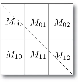
cores). In order to release that constraint, we decompose an N_×N matrix to m_×n block decomposition,

where m is the number of block rows and n is the number of block columns, and the only constraint of the

decomposition is m_×n=p, where 1_≤m,n_≤p. Thus, each process requires only approximately 1/p of

the full memory requirements of SMACOF algorithm. Figure 3.1 illustrates how we decompose each N_×N

matrix with 6 processes and m=2,n=3. Without a loss of generality, we assume N%m=N%n=0 in

Figure 3.1.

A process Pk,0≤k<p (sometimes, we will use Pi j for matching Mi j) is assigned to one rectangular

block Mi jwith respect to the simple block assignment equation in (3.1):

k=i_×n+j (3.1)

where 0_≤i<m,0_≤j<n. For N_×N matrices, such as∆,V†,B(X[k]), and so on, each block Mi jis assigned

(44)

M

₀₀

_M

₀₁

_M

₀₂

[image:44.612.187.459.119.407.2]

M

₁₀

M

₁₁

_M

₁₂

Figure 3.1: An example of an N_×N matrix decomposition of parallel SMACOF with 6 processes and 2_×3 block decomposition. Dashed line represents where diagonal elements are.

dimension, each process has a full N_×L matrix because these matrices have a relatively smaller size, and this

results in reducing the number of additional message passing routine calls. By scattering decomposed blocks

throughout the distributed memory, we are now able to run SMACOF with as huge a data set as the distributed

memory will allow concerning the cost of message passing overheads and a complicated implementation.

Although we assume N%m=N%n=0 in Figure 3.1, there is always the possibility that N%m₆=0 or

N%n₆=0. In order to achieve a high load balance under the N%m₆=0 or N%n₆=0 cases, we use a simple

modularoperation to allocate blocks to each process with at most ONE row or column difference between

them. The block assignment algorithm is illustrated in Algorithm 3.1.

At the iteration k in Algorithm 2.2, the application should acquire up-to-date information of the following

(45)

Algorithm 3.1 Pseudo-code for block row and column assignment for each process for high load balance.

Input: pNum, N, myRank

1: if N%pNum=0 then

2: nRows = N / pNum;

3: else

4: if myRank_≥(N%pNum)then

5: nRows = N / pNum;

6: else

7: nRows = N / pNum + 1;

8: end if

9: end if

10: return nRows;

feature of the SMACOF algorithm is that some of matrices are invariable, i.e.∆and V†, through the iteration. On the other hand, B(X[k−1])and STRESS (σ[k]) value keep changing at each iteration, since X[k−1]and X[k]

are changed in every iteration. In addition, in order to update B(X[k−1])and the STRESS (σ[k]) value in

each iteration, we have to take the N_×N matrices’ information into account, so that related processes should

communicate via MPI primitives to obtain the necessary information. Therefore, it is necessary to design

message passing schemes to do parallelization for calculating the B(X[k−1]₎_{and STRESS (}_σ[k]_{) values as}

well as the parallel matrix multiplication in Line 8 in Algorithm 2.2.

Computing the STRESS (Eq. (3.2)) can be implemented simply by a partial error sum of Di j and∆i j

followed by anMPI_Allreduce:

σ(X) =

∑

i<j≤N

wi j(di j(X)−δi j)2 (3.2)

where 1_≤i< j_≤N and wi jis a weight value, so wi j≥0. On the other hand, calculation of B(X[k−1]), as

shown at Eq. (2.16), and parallel matrix multiplication are not simple, especially for the case of m₆=n.

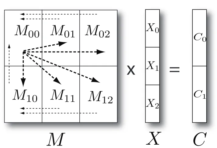
Figure 3.2 depicts how parallel matrix multiplication applies between an N_×N matrix M and an N_×L

matrix X. Parallel matrix multiplication for SMACOF algorithm is implemented in a three-step process

SCALABLE HIGH PERFORMANCE MULTIDIMENSIONAL SCALING

SCALABLE HIGH PERFORMANCE MULTIDIMENSIONAL

SCALING

Seung-Hee Bae

Copyright c

2012

Seung-Hee Bae

Acknowledgements

Seung-Hee Bae

SCALABLE HIGH PERFORMANCE MULTIDIMENSIONAL SCALING

Contents

List of Tables

List of Figures

1

Introduction

1.1

Introduction

1.2

Multidimensional Scaling (MDS)

∑

∑

1.3

Motivation

1.4

The Research Problem

1.5

Contributions

1.6

Dissertation Organization

2

Backgrounds

2.1

Classical Multidimensional Scaling

2.2

Scaling by a MAjorizing of a COmplicated Function (SMACOF)

2.3

Message Passing Interface (MPI)

2.4

Threading

2.5

Deterministic Annealing (DA)

3

High Performance Multidimensional Scaling

3.1

Overview

3.2

High Performance Visualization

3.2.1

Parallel SMACOF

M

00

M

01

M

02

M

10

M

11

M

12

∑

₀₀

_M

₀₁

_M

₀₂

₁₀

₁₁

_M

₁₂