https://doi.org/10.5194/bg-16-2049-2019 © Author(s) 2019. This work is distributed under the Creative Commons Attribution 4.0 License.
Modelling land–atmosphere daily exchanges of NO, NH
3
, and CO
2
in a semi-arid grazed ecosystem in Senegal
Claire Delon1, Corinne Galy-Lacaux1, Dominique Serça1, Erwan Personne2, Eric Mougin3, Marcellin Adon1,6, Valérie Le Dantec4, Benjamin Loubet2, Rasmus Fensholt5, and Torbern Tagesson5
1Laboratoire d’Aérologie, Université de Toulouse, CNRS, UPS, Toulouse, France
2UMR ECOSYS, INRA, AgroParisTech, Université Paris-Saclay, 78850, Thiverval-Grignon, France 3Géosciences Environnement Toulouse, Université de Toulouse, CNES, CNRS, IRD, UPS, Toulouse, France 4Centre d’Etudes Spatiales de le BIOsphère, Université de Toulouse, CNES, CNRS, IRD, UPS, Toulouse, France 5Department of Geosciences and Natural Resource Management, University of Copenhagen, Copenhagen, Denmark 6Laboratoire de Physique de l’Atmosphère, et de Mécanique des Fluides, Université Félix Houphouët-Boigny, Abidjan, Côte d’Ivoire
Correspondence:Claire Delon (claire.delon@aero.obs-mip.fr) Received: 30 July 2018 – Discussion started: 27 August 2018
Revised: 19 April 2019 – Accepted: 24 April 2019 – Published: 15 May 2019
Abstract. Three different models (STEP–GENDEC– NOflux, Zhang2010, and Surfatm) are used to simulate NO, CO2, and NH3 fluxes at the daily scale for 2 years (2012–2013) in a semi-arid grazed ecosystem at Dahra (15◦2401000N, 15◦2505600W, Senegal, Sahel). Model results are evaluated against experimental results acquired during three field campaigns. At the end of the dry season, when the first rains re-wet the dry soils, the model STEP–GENDEC– NOflux simulates the sudden mineralization of buried litter, leading to pulses in soil respiration and NO fluxes. The contribution of wet season fluxes of NO and CO2 to the annual mean is respectively 51 % and 57 %. NH3fluxes are simulated by two models: Surfatm and Zhang2010. During the wet season, air humidity and soil moisture increase, leading to a transition between low soil NH3 emissions (which dominate during the dry months) and large NH3 deposition on vegetation during wet months. Results show a great impact of the soil emission potential, a difference in the deposition processes on the soil and the vegetation between the two models with however a close agreement of the total fluxes. The order of magnitude of NO, NH3, and CO2fluxes is correctly represented by the models, as well as the sharp transitions between seasons, specific to the Sahel region. The role of soil moisture in flux magnitude is highlighted, whereas the role of soil temperature is less obvious. The simultaneous increase in NO and CO2 emissions and NH3
deposition at the beginning of the wet season is attributed to the availability of mineral nitrogen in the soil and also to microbial processes, which distribute the roles between respiration (CO2 emissions), nitrification (NO emissions), volatilization, and deposition (NH3 emission/deposition). The objectives of this study are to understand the origin of carbon and nitrogen compounds exchanges between the soil and the atmosphere and to quantify these exchanges on a longer timescale when only a few measurements have been performed.
1 Introduction
Sa-hel), the first rainfall events of the wet season cause strong pulses of CO2, N2O, NO, and NH3to the atmosphere (Jaeglé et al., 2004; McCalley and Sparks, 2008; Delon et al., 2015; Shen et al., 2016; Tagesson et al., 2016b). Anthropogenic ac-tivities have a strong impact on N and C cycling, and in large parts of the world, deposition of N compounds has several damaging impacts on ecosystem functions, such as changes in species biodiversity (Bobbink et al., 2010). The Sahel is still a protected region from this N pollution (Bobbink et al., 2010), but climate change could create an imbalance in bio-geochemical cycles of nutrients (Delgado-Baquerizo et al., 2013).
The emission of NO from soils leads to the formation of N2O and O3in the troposphere. Soil NO biogenic emissions from the African continent expressed in teragrammes of ni-trogen per year are considered as the largest in the world (Fowler et al., 2015) because of extended natural areas. The pulses of NO from the Sahel region at the beginning of the wet season have been shown to strongly influence the overly-ing N2O tropospheric column (Jaegle et al., 2004; Hudman et al., 2012; Zörner et al., 2016), indicating the urgent need for improved understanding of the dynamics of NO pulses from this region. NH3emissions lead to the formation of particles in the atmosphere, such as ammonium nitrates (NH4NO3), whose vapour phase dissociation further produces NH3and HNO3(Fowler et al., 2015). The land–atmosphere exchange of ammonia varies in time and space depending on environ-mental factors such as climatic variables, soil energy bal-ance, soil characteristics, and plant phenology (Flechard et al., 2013). Emissions of these compounds involve changes in atmospheric composition (ozone and aerosol production) and effects on climate through greenhouse gas impacts.
The N exchange fluxes are also influenced by the soil N content, and the main inputs of N compounds into the soil in semi-arid uncultivated regions are biological nitrogen fix-ation (BNF), decomposition of organic matter (OM), and at-mospheric wet and dry deposition (Perroni-Ventura et al., 2010). Soil N losses to the atmosphere involve N2O, NH3, and NO gaseous emissions, whereas within the soil, N can be lost via erosion, leaching, and denitrification. NO emissions to the atmosphere are mainly the result of nitrification pro-cesses, which is the oxidation of NH+4 to nitrates (NO−3) via nitrites (NO−2) through microbial processes (Pilegaard et al., 2013; Conrad, 1996). In remote areas, where anthropogenic emissions such as industrial or traffic pollution do not hap-pen, NH3bidirectional exchanges are regulated through di-verse processes: NH3 is emitted by livestock excreta, soil, and litter and is regulated by the availability of NH+4 and NH3in the aqueous phase (NHx), by the rate of
mineraliza-tion of NH+4, and by the availability of water, which allows NHx to be dissolved, to be taken up by organisms, and to
be released through decomposition (Schlesinger et al., 1991; Sutton et al., 2013). Additionally NH3 can be dry and wet deposited on soil and litter (Laouali et al., 2012; Vet et al., 2014), leaf cuticles, and stomata and regulated by chemical
interactions within the canopy air space (Loubet et al., 2012). The N cycle is closely linked to the C cycle, and it has been suggested that C–N interactions may regulate N availability in the soil (Perroni-Ventura et al., 2010). The link between N and C cycles in the soil, and their effects on OM decom-position, affect the emissions of C and N compounds to the atmosphere. These cycles are interlinked by respiration and decomposition processes in the soil, and the balance between C and N is controlled by biological activity, mainly driven by water availability in drylands (Delgado-Baquerizo et al., 2013). Indeed, the decomposition of soil OM, and its effi-ciency, regulates the amount of CO2 that is released to the atmosphere (Elberling et al., 2003).
Biogeochemical regional models have been applied for N compound emissions mostly in temperate regions (Butterbach-Bahl et al., 2001, 2009), where the spatial and temporal resolution of data is well characterized. Global ap-proaches have also been developed, with a simplified de-scription of processes and with coarse spatial resolution (Yienger and Levy, 1995; Potter et al., 1996; Yan et al., 2005; Hudman et al., 2012). Considering the weak number of experimental data in semi-arid regions about trace gas ex-changes and their driving parameters, one-dimensional mod-elling is a complementary, essential, and alternative way of studying the annual cycle dynamics and the underlying pro-cesses of emission and deposition. The specificity of the semi-arid climate needs to be precisely addressed in the mod-els used to be able to correctly represent the pulses of emis-sions and the strong changes in C and N dynamics at the transition between seasons. Improving the description of pro-cesses in 1-D models in tropical regions is therefore a neces-sary step before implementing regional modelling.
2 Materials and methods
2.1 Field site
Measurements were performed at the Dahra field station, part of the Centre de Recherches Zootechniques (CRZ), in the Sa-helian region of Ferlo, Senegal (15◦2401000N, 15◦2505600W). The Dahra field site is located within the CRZ managed by the Institut Sénégalais de Recherche Agronomique (ISRA). This site is a semi-arid savanna used as a grazed rangeland. The Sahel is under the influence of the West African Mon-soon (cool wet southwesterly wind) and the Harmattan (hot dry northeasterly wind) depending on the season. Rainfall is concentrated in the core of the monsoon season, which ex-tends from mid-July to mid-October. At Dahra, the annual rainfall was 515 mm in 2012 and 356 mm in 2013 with an average of 416 mm for the period 1951–2013. The annual mean air temperature at 2 m height was 28.4◦C in 2012 and 28.7◦C in 2013, with an average of 29◦C for the period 1951–2003. The most abundant tree species are Balanites aegyptiaca andAcacia tortilis, and the herbaceous vegeta-tion is dominated by annual C4grasses (e.g.Dactyloctenium aegyptium,Aristida adscensionis,Cenchrus biflorus, and Er-agrostis tremula) (Tagesson et al., 2015a). Livestock is dom-inated by cows, sheep, and goats, and grazing occurs perma-nently all year-round (Assouma et al., 2017). This site was previously described in Tagesson et al. (2015b) and Delon et al. (2017).
2.2 Field data
2.2.1 Hydro-meteorological data and sensible and latent heat fluxes
A range of hydro-meteorological variables are measured by a meteorological station at the Dahra field site (Tagesson et al., 2015b). The hydro-meteorological variables used in this study were rainfall (mm), air temperature (◦C), relative air humidity (%), wind speed (m s−1), air pressure (hPa) at 2 m height, soil temperature (◦C), soil moisture (%) at 0.05, 0.10, and 0.30 m depth, and net radiation (W m−2). Data were sam-pled every 30 s and stored as 15 min averages (sum for rain-fall). Data have then been 3h and daily averaged for the pur-pose of this study.
Land–atmosphere exchanges of sensible and latent heat was measured for the years 2012 and 2013 with an eddy co-variance system consisting of an open-path infrared gas an-alyzer (LI-7500, LI-COR Inc., Lincoln, USA) and a three-axis sonic anemometer (Gill R3 ultrasonic anemometer, Hampshire, UK) (Tagesson et al., 2015a). The sensors were mounted 9 m above the ground and data were collected at a 20 Hz rate. The post-processing was performed with the Ed-dyPro 4.2.1 software (LI-COR Biosciences, 2012) and statis-tics were calculated for 30 min periods. For a thorough
de-scription of the post-processing of sensible and latent heat fluxes, see Supplement of Tagesson et al. (2015b).
2.2.2 Atmospheric NH3concentrations using passive samplers
Atmospheric concentrations of NH3 and other compounds such as N2O, HNO3, O3, and SO2 were measured using passive samplers on a monthly basis, in accordance with the methodology used within the INDAAF (International Network to study Deposition and Atmospheric chemistry in Africa) program (https://indaaf.obs-mip.fr, last access: 8 May 2019) driven by the Laboratoire d’Aerologie (LA) in Toulouse. While not being actually part of the INDAAF network, the Dahra site was equipped with the same passive sampler devices and analyses of these samplers were per-formed following the INDAAF protocol at LA.
Passive samplers were mounted under a stainless-steel holder to avoid direct impact from wind transport and splash-ing from precipitation. The holder was attached at a height of about 1.5 m above ground. All the samplers were exposed in pairs in order to ensure the reproducibility of results. The samplers were prepared at LA in Toulouse, installed and col-lected after 1 month exposure by a local investigator, and sent back to LA. Samplers before and after exposition were stored in a fridge (4◦C) to minimize possible bacterial de-composition or other chemical reactions. Samplers were then analysed by ion chromatography (IC) to determine ammo-nium and nitrate concentrations. Validation and quality con-trol of passive samplers according to international standards (World Meteorological Organization report), as well as the sampling procedure and chemical analysis of samples, have been widely detailed in Adon et al. (2010). Monthly mean NH3concentrations in parts per billion by volume are calcu-lated for the period 2012 and 2013. The measurement accu-racy of NH3passive samplers, evaluated through covariance with duplicates, and the detection limit evaluated from field blanks were estimated respectively at 14 % and 0.7±0.2 ppb (Adon et al., 2010).
2.2.3 Measurements of NO, NH3, and CO2
(respiration) fluxes from soil and soil physical parameters
NO and NH3 fluxes were measured with a manual closed dynamic Teflon chamber (non-steady-state through-flow chamber; Pumpanen et al., 2004) with dimensions of 200 mm width×400 mm length×200 mm height. During the J12 campaign, the chamber was connected to a Labo-ratoire d’Aerologie analyzer, whereas in J13 and N13, it was connected to a Thermo Scientific 17I analyzer (ThermoFis-cher Scientific, MA, USA). The calculation of fluxes is based on an equation detailed in Delon et al. (2017), adapted from Davidson et al. (1991). The increase rate of NO and NH3 mixing ratios used in the flux calculation equation was esti-mated by a linear regression fitted to data measured for 180 to 300 s for NO (120 s for NH3) following the installation of the chamber on the soil, as detailed in Delon et al. (2017). Close to the Teflon chamber, soil CO2 respiration was measured with a manual closed dynamic chamber (SRC-1 from PP Systems, 150 mm height×100 mm diameter) coupled to a non-dispersive infrared CO2/H2O analyzer EGM-4 (PP Sys-tems, Hitchin, Hertfordshire, UK). Soil CO2respiration was measured within 30 cm of the location of the NO and NH3 fluxes. Measurements were performed on bare soil to ensure only root and microbe respiration. Results of NO, NH3, and CO2 fluxes are presented as daily means with daily stan-dard deviations. Along with flux measurements, soil physi-cal parameters were measured during the campaigns: soil pH ranges from 5.77 to 7.43, sand content ranges between 86 % and 94 %, and clay content ranges between 4.7 % and 7.9 %. All the methods, calculations, and results from the field cam-paigns are fully detailed in Delon et al. (2017).
2.3 Modelling biogenic NO fluxes, CO2respiration, and ammonium content in
STEP–GENDEC–NOflux
2.3.1 The STEP–GENDEC model
The STEP model is presented in Appendix A, with forcing variables detailed in Table A1, site parameters used in the ini-tialization in Table A2, numerical values of parameters used in the equations in Table A3, and equations, variables, pa-rameters, and constants used in the equations in Table A4.
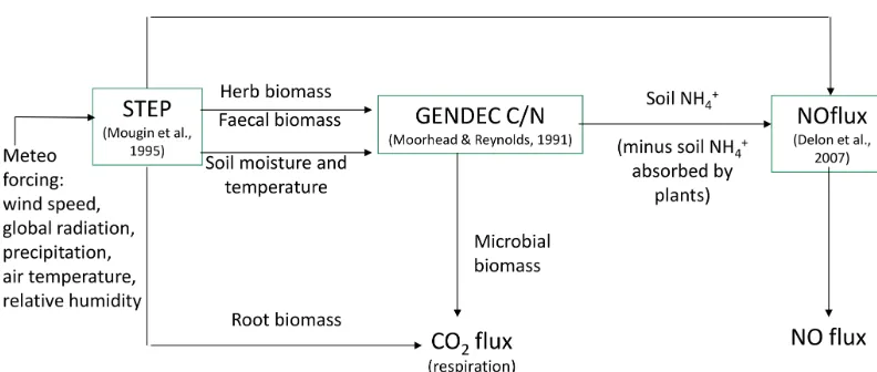
STEP is an ecosystem process model for Sahelian herba-ceous savannas (Mougin et al., 1995; Tracol et al., 2006; Delon et al., 2015). It is coupled to GENDEC, which aims at representing the interactions between litter, decomposer microorganisms, microbial dynamics, and C and N pools (Moorhead and Reynolds, 1991). It simulates the decom-position of the organic matter and microbial processes in the soil in arid ecosystems. Information such as the quan-tity of organic matter from faecal matter from livestock and herbal masses is transferred from STEP as inputs to GEN-DEC (Fig. 1).
Soil temperatures are simulated from air temperature ac-cording to Parton (1984). This model requires daily maximal and minimal air temperature, global radiation (provided by
forcing data), herbaceous aboveground biomass (provided by the model), initial soil temperature, and soil thermal diffusiv-ity. Details of equations are given in Delon et al. (2015) and Appendix A (Tables A3 and A4).
Soil moisture values are calculated following the tipping-bucket approach (Manabe, 1969): when the field capacity is reached, the excess water in the first layer (0–2 cm) is trans-ferred to the second layer, between 2 and 30 cm. Two other layers are defined, between 30–100 cm and 100–300 cm. Equations related to soil moisture calculation are detailed in Appendix A (Table A4) and in Jarlan et al. (2008). This ap-proach, while being simple in its formulation, is especially useful in regions where detailed description of the environ-ment is not available or unknown, and where the natural het-erogeneity of the soil profile is high due to the presence of di-verse matter fragments such as buried litter, dead roots from herbaceous mass and trees, stones, branches, and tunnels dug by insects and little mammals.
The STEP model is forced daily by rain, global radiation, air temperature, wind speed, and relative air humidity at 2 m height. Initial parameters specific to the Dahra site are listed in Table A1 and site parameters in Table A2.
2.3.2 Respiration and biogenic NO fluxes
The quantity of carbon in the soil was calculated from the total litter input from faecal and herbal mass, where faecal matter is obtained from the number of livestock heads graz-ing at the site (Diawara, 2015; Diawara et al., 2018). The quantity of carbon is 50 % the buried litter mass. The carbon and nitrogen exchanges between pools and all equations are detailed in Moorhead and Reynolds (1991) and will not be developed here. Carbon dynamics depend on soil tempera-ture, soil moistempera-ture, and soil nitrogen (linked to microbial dy-namics). The concentration of nitrogen in the soil is derived from the quantity of carbon using C/N ratios.
Biogenic NO fluxes were calculated using the coupled model STEP–GENDEC–NOflux, as detailed in Delon et al. (2015). The NOFlux model uses an artificial neural net-work approach to estimate the biogenic NO emission from soil to the atmosphere (Delon et al., 2007, 2015). The NO flux is calculated from and depends on parameters such as soil surface temperature and moisture, soil temperature at 30 cm depth, sand percentage, N input (here given as a per-centage of the ammonium content in the soil), wind speed, and soil pH. The input of N to the soil from the buried litter is provided by STEP, and the calculation of the ammonium content in the soil coming out from this N input is provided by GENDEC. The equations used for NO flux calculation are reported in Appendix B, taken from Delon et al. (2015).
Figure 1.Schematic representation of NO and CO2flux modelling in STEP–GENDEC–NOflux (adapted from Delon et al., 2015).
calculation. In the current version, the NO emitted to the at-mosphere results from 1 % of the NH+4 pool in the soil minus the N absorbed by plants. The percentage of soil NH+4 pool used to calculate the NO emission has been changed from 2 % to 1 % based on Potter et al. (1996), who proposed a range between 0.5 % and 2 %. In the present study, the 1 % value was more adapted to fit experimental values.
Soil respiration is the sum of autotrophic (root only) and heterotrophic respiration. The autotrophic respiration in STEP is calculated from growth and maintenance respira-tions of roots and shoots (Mougin et al., 1995), following equations reported in Table A4. Autotrophic respiration de-pends on root depth soil moisture and soil temperature (2– 30 cm) and root biomass, whose dynamics are simulated by STEP. The heterotrophic respiration is calculated in GEN-DEC from the growth and death of soil microbes in the soil depending on the available litter C (given by STEP). Micro-bial respirationρin grammes of carbon per day is calculated as in Eq. (1).
ρ=(1−ε)Ca (1)
Microbial growth in grammes of carbon per day isγ=εCa, whereεis the assimilation efficiency (unitless) and Ca is total C available in grammes of carbon per day, i.e. total C losses from four different litter inputs, buried litter, litter from trees, faecal matter, and dry roots. Microbial death is driven by the death of the living microbe mass, and the change in water po-tential during drying–wetting cycles (change between −1.5 and −0.01 MPa in the layer 2–30 cm). These calculations are described in Moorhead and Reynolds (1991) and Delon et al. (2015) and are not reported in detail in this study. A schematic view of STEP–GENDEC–NOFlux is presented in Fig. 1. Simulated variables and corresponding measurements used for validation are summarized in Table 1.
2.4 Modelling NH3fluxes
The net NH3flux between the surface and the atmosphere depends on the concentration differenceχcp−CNH3 , where CNH3 is the ambient NH3 concentration in microgrammes
per cubic metre, andχcpis the concentration of the canopy compensation point in microgrammes per cubic metre. The canopy compensation point concentration is the atmospheric NH3 concentration in the canopy for which the fluxes be-tween the soil, the stomatal cavities, and the air inside the canopy switch from emission to deposition, or vice versa (Farquhar et al., 1980; Wichink Kruit et al., 2007). The canopy compensation point concentration takes into account the stomatal and soil layers. The soil compensation point concentration, χg, in parts per billion has been calculated from the emission potential0g(unitless) as a function of soil surface temperatureTgin kelvin according to Wentworth et al. (2014):
χg=13 587×0g×e−(10 396/Tg)×109. (2) A large0gindicates that the soil has a high propensity to emit NH3, considering that the potential emission of NH3depends on the availability of ammonium in the soil and on the pH. 0g= [NH+4]/[H+]concentrations were measured in the field and are available in Delon et al. (2017).
Two different models designed to simulate land– atmosphere NH3 bidirectional exchange are used in this study and described below.
2.4.1 Inferential method (Zhang et al., 2010)
An inferential method was used to calculate the bidirectional exchange of NH3. The overall flux FN H3(µg m−2s−1) is cal-culated as
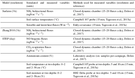
Table 1.Summary of different models used in the study, with the variables simulated and compared to measurements. All simulated and measured variables were daily averaged for the purpose of the study.
Model (resolution) Simulated and measured variables (units)
Methods used for measured variables (resolution and reference)
Surfatm (3 h) NH3bidirectional fluxes
(ngN m−2s−1)
Closed dynamic chamber (15–20 fluxes a day, Delon et al., 2017)
Soil surface temperature (◦C) Campbell 107 probe (15 min, Tagesson et al., 2015a) Sensible and latent heat fluxes (W m−2) Eddy covariance (15 min, Tagesson et al., 2015a) Zhang2010 (3 h) NH3bidirectional fluxes
(ngN m−2s−1)
Closed dynamic chamber (15–20 fluxes a day, Delon et al., 2017)
STEP (day) NO biogenic fluxes (ngN m−2s−1)
Closed dynamic chamber (15–20 fluxes a day, Delon et al., 2017)
CO2respiration fluxes
(ngN m−2s−1)
Closed dynamic chamber (15–20 fluxes a day, Delon et al., 2017)
Ammonium content (%) Laboratory analysis (six samples per campaign, Delon et al., 2017)
Soil temperature at two depths: 0–2 and 2–30 cm (◦C)
Campbell 107 probe at two depths: 5 and 10 cm (15 min, Tagesson et al., 2015a)
Soil moisture at two depths: 0–2 and 2–30cm (%)
HH2 Delta probe at two depths: 5 and 10 cm (15 min, Tagesson et al., 2015a)
with Vd= 1/(Ra+Rb+Rc), where Vd (m s−1) is the position velocity, determined by using the big-leaf dry de-position model of Zhang et al. (2003). Ra (s m−1) and Rb (s m−1) are the aerodynamic and quasi-laminar resistances respectively, andRc(s m−1) is the total resistance to deposi-tion resulting from component terms such as stomatal, mes-ophyll, and non-stomatal/external/cuticular and soil resis-tances (Flechard et al., 2013, and references therein).CNH3
(µg m−3) is determined at the monthly scale from passive sampler measurements. Theχcpterm (µg m−3) is calculated following the two-layer Zhang et al. (2010) model, hereafter referred to as Zhang2010. This model gives access to an ex-tensive literature review on compensation point concentra-tions and emission potential values classified for 26 different land use classes (LUCs). Compensation point concentrations are calculated in the model and vary with canopy type, nitro-gen content, and meteorological conditions. This model was adapted by Adon et al. (2013) for the specificity of semi-arid ecosystems such as leaf area index (LAI) or type of vege-tation, assuming a ground emission potential of 400 (unit-less), considered a low-end value for non-fertilized ecosys-tems according to Massad et al. (2010) and based on De-lon et al. (2017) experimental results, and a stomatal emis-sion potential of 100 (unitless) based on Massad et al. (2010) for grass, and on the study of Adon et al. (2013) for simi-lar ecosystems as the one found in Dahra. Considering the bidirectional nature of NH3exchange, emission occurs if the canopy compensation point concentration is superior to the
ambient concentration (Nemitz et al., 2001). Emission fluxes are noted as positive. Meteorological forcing required for the simulation is 3 h-averaged wind speed, net radiation, pres-sure, relative humidity, air temperature at 2 m height, surface temperature at 5 cm depth, and rainfall. The equations used in this model are extensively described in Zhang et al. (2003, 2010), and will not be detailed here.
2.4.2 The Surfatm model
The model is forced every 3 h by net radiation, deep soil temperature (30 cm), air temperature, relative humidity, wind speed, rainfall, and atmospheric NH3 concentration with monthly values from passive sampler measurements repeated every 3 h. Forcing also includes values of leaf area index (LAI, measured), canopy height Zh (estimated), roughness length Z0(0.13Zh), displacement heightD(0.7Zh), stom-atal emission potential (constant), ground emission potential (derived from measurements during field campaigns, con-stant the rest of the time), and measurement heightZref(2 m). LAI was measured according to the methodology developed in Mougin et al. (2014). Data from Dahra were measured monthly during the wet season and were not published (Mou-gin, personal communication). Linear interpolation was per-formed between these monthly estimates, and values for the dry season were found in Adon et al. (2013), for an equiv-alent semi-arid ecosystem in Mali, derived from MODIS (Moderate-Resolution Imaging Spectroradiometer) measure-ments. The ground emission potential has been set to 400 (unitless), and the stomatal emission potential has been set to 100 (unitless) as in the simulation based on Zhang2010, ex-cept during field campaign periods, where the ground emis-sion potential was derived from experimental values (700 in J12 and J13 and 2000 in N13). In Table 2, constant input pa-rameters are listed. Some of them were adapted to semi-arid conditions to get the best fit between measured and simulated fluxes, specified in Table 2.
The main difference between Surfatm and Zhang2010 is the presence of a SVAT (surface vegetation atmosphere trans-fer) model in Surfatm (Personne et al., 2009), allowing for energy budget consideration and accurate restitution of sur-face temperature and moisture. Simulated variables and cor-responding measurements used for validation are summa-rized in Table 1.
2.5 Statistic analysis
The R software (http://www.R-project.org, last access: 8 May 2019) was used to provide results of simple and mul-tiple linear regression analysis. The cor.test() function was used to test a single correlation coefficient R, i.e. a test for association between paired samples, using one of Pear-son’s product moment correlation coefficients. Thep value is used to determine the significance of the correlation. If the p value is less than 0.05, the correlation is considered non-significant. The lm() test was used for stepwise multiple regression analysis. The adjustedRsquared (i.e. normalized multipleRsquared,R2), determines how well the model fits to the data. Again, the p value is calculated, and has to be less than 0.05 to give confidence in the significance of the determination coefficientR2. These tests are used in the fol-lowing paragraphs (i) to determine if the models are precise enough to correctly represent environmental variables like soil moisture, soil temperature, and latent and sensible heat fluxes at the annual scale and to represent measured fluxes
of NO, NH3, and CO2 for some periods (ii) to verify if en-vironmental drivers, taken individually or in groups, explain the NO/NH3/CO2simulated fluxes and to what extent and (iii) to compare the two models used for NH3flux modelling.
3 Results
3.1 Soil moisture, soil temperature, and land–atmosphere heat fluxes
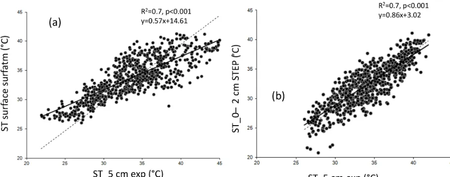
Soil moisture simulated by STEP in the surface layer (Fig. 2a) is limited at 11 % during the wet season. This value corresponds to the field capacity calculated by STEP. The soil moisture modelling follows the tipping-bucket approach; i.e. when the field capacity is reached, the excess water is trans-ferred to the second layer, between 2 and 30 cm. Experimen-tal values measured at 5 and 10 cm are better represented by the model in this second layer (Fig. 2b). Linear regression gives aR2of 0.74 (resp. 0.81), a slope of 0.98 (resp. 1.05), and an offset of 0.34 (resp. 0.32) between STEP soil mois-ture in the 0–2 cm (resp. 2–30 cm) layer and experimental soil moisture at 5 cm.R2is 0.77, slope is 0.93, and offset is 0.84 between STEP soil moisture in the 2–30 cm layer and experimental soil moisture at 10 cm. The temporal dynamics given by STEP, the filling of the surface layer, and the maxi-mum and minimaxi-mum values are comparable to the data. How-ever, the drying of the layers is sharper in the model than in measurements at the end of the wet season, leading to an un-derestimation of the model compared to measurements until December each year.
As a comparison, linear correlation between STEP H (STEP LE) and EC H (EC LE) givesR2of 0.4 (0.7), for both years of simulation (Fig. 3a and b). The significant correla-tion between Surfatm and EC latent heat fluxes indicates that the stomatal, aerodynamic, and soil resistances are correctly characterized in the model, giving confidence in the further realistic parameterization of NH3fluxes, despite missing val-ues in intermediate fluxes, due to the criteria applied by the post-processing (see Supplement of Tagesson et al., 2015b).
Surfatm soil surface temperature is very close to mea-sured soil surface temperature (Fig. 4a,R2=0.70,p<0.001 in 2012–2013). Mean annual values were 35.8 and 34.2◦C respectively for surface Surfatm and measured soil surface temperatures in 2012 and 32.4 and 33.8◦C in 2013. STEP surface temperatures (0–2 cm layer) present mean values of 32.0◦C in 2012 and 32.6◦C in 2013. Linear regression be-tween STEP surface temperature and measured surface tem-perature (Fig. 4b) gives a R2 of 0.7 (p<0.001) for 2012– 2013. Slopes and offsets are indicated in the figures.
3.2 Biogenic NO fluxes from soil and ammonium content
respec-Table 2.Input parameters for the Surfatm model. Ranges refer to Hansen et al. (2017). All measured parameters refer to Delon et al. (2017).
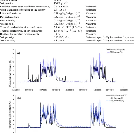
Description of parameters in Surfatm Value in this study (range) Sources
Time step 3 h
Characteristic length of leaves 0.03 m (0.03–0.5) Minimum value Total soil depth 0.92 m
Soil density 1500 kg m−3
Radiation attenuation coefficient in the canopy 0.7 (0.5–0.8) Estimated Wind attenuation coefficient in the canopy 2.3 (1.5–5) Estimated Initial soil moisture 0.09 kg(H2O) kg(soil)−1 Measured Dry soil moisture 0.02 kg(H2O) kg(soil)−1 Measured
Field capacity 0.14 kg(H2O) kg(soil)−1 Measured Wilting point 0.02 kg(H2O) kg(soil)−1 Measured
Thermal conductivity of wet soil layers 2.5 W m−1K−1(1.6–2.2) Estimated Thermal conductivity of dry soil layers 1.5 W m−1K−1(0.2–0.3) Estimated Depth of temperature measurements 0.3 m Measured
Soil porosity 0.45 (0.25–0.4) Estimated specifically for semi-arid ecosystems Soil tortuosity 2.5 (2–4) Estimated specifically for semi-arid ecosystems
Figure 2. (a)Volumetric soil moisture simulated by STEP in the first layer (0–2 cm) in black and soil moisture measured at 5 cm in blue, as a percentage, at a daily scale.(b)Volumetric soil moisture simulated by STEP in the second layer (2–30 cm) in black, soil moisture measured at 5 cm as a blue solid line, measured at 10 cm as a blue dotted line, as a percentage, at a daily scale.
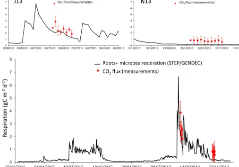
tively. In J13, average NO fluxes are 10.3±3.3 and 5.1± 2.1 ngN m−2s−1 for modelled and measured fluxes respec-tively. In N13, average NO fluxes are 2.2±0.3 and 4.0± 2.2 ngN m−2s−1 for modelled and measured fluxes respec-tively. Emission fluxes are noted as positive.
[image:8.612.70.523.135.585.2]Figure 3. (a)Daily modelled latent heat flux in Surfatm vs. daily measured latent heat flux, in watts per square metre;(b)daily modelled sensible heat flux in Surfatm vs. daily measured sensible heat flux, in watts per square metre. The thick black line is for the linear regression, and the dashed black line is the 1:1 line. Available measured EC data are more numerous for H than for LE due to the criteria applied by the post-processing (see Supplement of Tagesson et al., 2015b).
Figure 4. (a)Modelled daily surface temperature in Surfatm vs. measured daily temperature at 5 cm depth;(b)modelled daily surface temperature in STEP (0–2 cm layer) vs. measured daily temperature at 5 cm depth. The thick black line is for the linear regression, and the dashed black line is the 1:1 line.
al. (2017), showing an overestimation of released N during the J13 wet season and an underestimation at the end of the wet season (as N13).
Modelled dry and wet season NO fluxes are respec-tively 2.5±2.5 and 6.2±4.1 ngN m−2s−1 for both 2012 and 2013, and the simulation gives a mean flux of 3.6± 2.9 ngN m−2s−1 for the entire study period. Wet season fluxes represent 51 % of the annual mean, even though it only lasts 3 to 4 months. Simulated NO fluxes are signifi-cantly correlated with measured soil moisture at 5 cm depth (R2=0.42,p<0.001, slope=0.65, offset=0.69) and 10 cm depth (R2=0.43,p<0.001, slope=0.72, offset=0.33) for both years, but not directly with soil temperature. A multi-ple linear regression model involving soil moisture at 5 cm
[image:9.612.72.527.64.235.2] [image:9.612.71.526.307.486.2]Figure 5.Daily NO flux simulated by STEP–GENDEC–NOFlux (ngN m−2s−1, black line) and daily averaged NO flux measurements during the three field campaigns (red triangles). Error bars in red give the standard deviation for measurements at the daily scale. Rain is represented by the blue line in millimetres in the bottom panel. The upper panels show a focus on each field campaign.
[image:10.612.62.533.417.687.2]3.3 Soil CO2respiration
Soil respiration includes soil heterotrophic respiration, which refers to the decomposition of dead soil organic matter (SOM) by soil microbes, and root respiration, including all respiratory processes occurring in the rhizosphere (Xu et al., 2016). The simulated respiration of aboveground biomass is not included as in measured data.
In J13, the average measured flux is 2.6±0.6 gC m−2d−1, and the average modelled flux is 1.9±0.4 gC m−2d−1. The correlation between the two data sets is not significant. In N13, the average measured flux is 0.78±0.11 gC m−2d−1, and the average modelled flux is 0.18±0.02 gC m−2d−1. The two data sets are not correlated. November fluxes are less important than July fluxes, as illustrated by both the model and the measurements (Fig. 7), and as previously shown with eddy covariance data (Tagesson et al., 2015a). Simulated res-piration fluxes are in the range of measured fluxes in J13, but appear to underestimate measured fluxes in N13 (Fig. 7). The simulated autotrophic respiration (roots+aboveground biomass) is shown, together with the heterotrophic (mi-crobes) respiration, to check for a possible role of above-ground biomass in comparison with measurements (Fig. 8). As expected, the heterotrophic respiration is higher than the autotrophic respiration before and after the growth of the vegetation, i.e. at the beginning and end of the wet season in 2012, or during precipitation dry spells (e.g. in J13). At the end of the wet season, the late peaks of simulated het-erotrophic respiration are linked to late rain events because autotrophic respiration is no more effective when vegetation is not growing anymore. Adding the autotrophic respiration to the heterotrophic respiration does not help to better fit the measured respiration in N13.
Average dry and wet season simulated soil respiration are respectively 0.3±0.7 and 1.0±0.4 gC m−2d−1, while the annual mean is 0.5±0.7 gC m−2d−1. This annual mean is below global estimates for grassland (2.2 gC m−2d−1) and deserts partially vegetated (1.0 gC m−2d−1; Xu et al., 2016). The wet season has the largest contribution (57 %) to the an-nual respiration budget (with wet seasons of 114 and 81 d in 2012 and 2013 respectively).
Simulated daily respiration from microbes and roots is significantly correlated with measured soil moisture at 5 cm depth withR2=0.50,p<0.001, slope=0.17, offset=0.26 and 10 cm depth withR2=0.5,p<0.001, slope=0.19, off-set= −0.37 for both years, whereas soil field-measured res-piration shows a lower correlation with surface soil moisture, withR2=0.4,p=0.09, slope=0.03, offset= −0.07 in J13 andR2=0.3,p=0.1, slope=0.02, offset= −0.02 in N13.
3.4 NH3bidirectional exchange
NH3fluxes were simulated by two different models: Surfatm (Personne et al., 2009) and Zhang2010 (Fig. 9). The same ambient concentrations deduced from in situ measurements
are prescribed in both models. Average fluxes are reported in Table 2. In J12, simulated fluxes are not significantly corre-lated with measured data. In J13, Surfatm and measurement fluxes are not significantly correlated (R2=0.2 p=0.2). In N13, Surfatm and measured fluxes are not significantly correlated (R2=0.2, p=0.2), and Zhang2010 and mea-sured fluxes are significantly correlated (R2=0.5,p=0.01, slope=1.5, offset= −3.8).
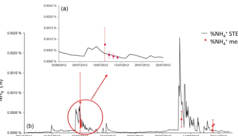
Figure 9 shows alternative changes between low NH3 emission and low deposition. This switch occurs during the dry seasons (from mid-October to the end of June). Indeed, monthly averaged compensation point and ambient concen-tration values are quite similar during the dry seasons. Com-pensation point concentration averaged during the 2012 and 2013 dry seasons is 3.8±1.5 ppb, and averaged ambient con-centration is 4.3±1.5 ppb for the same period. If the 2012 and 2013 dry seasons are considered separately, the values of the means remain the same. Low deposition dominates when air humidity is sufficiently high, roughly above 25 % (before and after the wet season), whereas low emission dominates when air humidity is low (< 25 %).
The net dry and wet season fluxes reported in Table 3 are in a similar range as NH3 fluxes calculated by Adon et al. (2013) using Zhang2010 at comparable Sahelian sites in Mali and Niger. NH3 fluxes ranged between −3.2 and 0.9 ngN m−2s−1 during the dry season and between−14.6 and−6.0 ngN m−2s−1during the wet season.
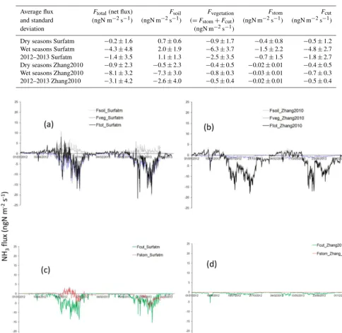
Figure 10 shows the partition between the different contri-butions of soil and vegetation to the NH3 fluxes in Surfatm and Zhang2010. During the wet season, the contributions of vegetation and soil in Surfatm (Zhang2010) are−6.3± 3.7 (−0.8±0.36 ngN m−2s−1) and 2.0±1.9 ngN m−2s−1 (−7.3±3.0 ngN m−2s−1) respectively for both years. Dur-ing the dry season, vegetation (i.e. stomata+cuticles) and soil contributions are low: −0.9±1.7 and 0.7± 0.6 ngN m−2s−1respectively in Surfatm and−0.4±0.5 and −0.5±2.3 ngN m−2s−1 in Zhang2010, as reported in Ta-ble 4. In N13, at the end of the wet season, the soil con-tribution is 2.9±0.7 ngN m−2s−1in Surfatm, whereas it is −2.6±0.8 ngN m−2s−1in Zhang2010.
Figure 7.Daily root and microbe respiration in milligrammes of carbon per square metre per day simulated by STEP–GENDEC (black line), and daily averaged soil respiration measurements (red squares) during two field campaigns. Error bars in red give the standard deviation at the daily scale. The upper panels show a focus of J13 and N13 field campaigns.
[image:12.612.84.513.486.684.2]Figure 9.Daily NH3flux (ngN m−2s−1) simulated by Surfatm (black line) and Zhang2010 (grey dashed line) and daily averaged NH3flux
measurements during three field campaigns (red triangles). Error bars in red stand for standard deviation at the daily scale. Air humidity as a percentage (blue line). DS: dry season; WS: west season.
Table 3.Averaged NH3fluxes for measurements and the Surfatm and Zhang2010 models during specific periods. Measurements are available
during the three field campaigns and not at the annual or seasonal scale.
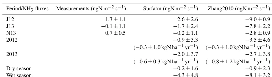
Period/NH3fluxes Measurements (ngN m−2s−1) Surfatm (ngN m−2s−1) Zhang2010 (ngN m−2s−1)
J12 1.3±1.1 2.6±2.6 −9.0±0.9 J13 −0.1±1.1 −1.7±2.4 −7.8±2.2 N13 0.7±0.5 −0.2±1.1 −2.8±0.9
2012 −0.9±3.3 −3.5±4.6
(−0.3±1.0 kgN ha−1yr−1) (−0.3±1.0 kgN ha−1yr−1)
2013 −2.0±3.7 −2.7±3.8
(−0.6±0.3 kgN ha−1yr−1) (−0.8±1.2 kgN ha−1yr−1)
Dry season −0.2±1.6 −0.9±2.3
Wet season −4.3±4.8 −8.1±3.2
On the basis of the different averages for each contributing flux in Table 4, we estimate that the soil is a net source of NH3during the wet season, while the vegetation is a net sink in Surfatm, and the soil is a net sink in Zhang2010.
4 Discussion
4.1 NH3exchanges
4.1.1 Relevance of monthly NH3concentration input vs. daily NH3flux outputs
In the two models, CNH3 used as input data arises from
passive sampler measurements, integrated at the monthly scale (see Sect. 2.2.2). Output fluxes are provided at a 3 h timescale, averaged at the daily scale for the purpose of this
[image:13.612.81.515.370.494.2]Table 4.Contributions of vegetation and soil to the total NH3flux in Surfatm and Zhang2010, wet season mean, dry season mean, and annual mean, for both years of simulation.
Average flux Ftotal(net flux) Fsoil Fvegetation Fstom Fcut
and standard (ngN m−2s−1) (ngN m−2s−1) (=Fstom+Fcut) (ngN m−2s−1) (ngN m−2s−1)
deviation (ngN m−2s−1)
Dry seasons Surfatm −0.2±1.6 0.7±0.6 −0.9±1.7 −0.4±0.8 −0.5±1.2 Wet seasons Surfatm −4.3±4.8 2.0±1.9 −6.3±3.7 −1.5±2.2 −4.8±2.7 2012–2013 Surfatm −1.4±3.5 1.1±1.3 −2.5±3.5 −0.7±1.5 −1.8±2.7 Dry seasons Zhang2010 −0.9±2.3 −0.5±2.3 −0.4±0.5 −0.02±0.01 −0.4±0.5 Wet seasons Zhang2010 −8.1±3.2 −7.3±3.0 −0.8±0.3 −0.03±0.01 −0.7±0.3 2012–2013 Zhang2010 −3.1±4.2 −2.6±4.0 −0.5±0.4 −0.02±0.01 −0.5±0.4
Figure 10.Daily NH3flux (ngN m−2s−1) partitioned between soil and vegetation. The black line is for total net flux (Ftot), the grey dashed
line is for soil flux (Fsol), and the blue line is for vegetation flux (Fveg) for Surfatm in(a)and for Zhang2010 in(b). The red line is for
stomatal flux (Fstom) and the green line is for cuticular flux (Fcut) for Surfatm in(c)and for Zhang2010 in(d).
valuable reason to use monthly concentrations as inputs in the present study.
4.1.2 NH3deposition flux variation
Dahra is a grazed savanna where the main source of NH3 emission to the atmosphere is the volatilization of livestock excreta (Delon et al., 2012); the excreta quantity and
August whereas the canopy compensation point remains sta-ble, the flux will decrease as shown by Eq. (3).
August is the month with the maximum ammonium wet deposition, which leads to a strong leaching of the atmo-sphere and explains the decrease in the NH3 concentration (Laouali et al., 2012).
4.1.3 Role of soil moisture and soil temperature in NH3 fluxes
A significant correlation is found between Zhang2010 fluxes and measured soil moisture at 5 cm depth (R2=0.6, p<0.01, slope= −1.2, offset=2.1) for 2012–2013. Surfatm fluxes and measured soil moisture at 5 cm depth are also sig-nificantly correlated with R2=0.3, p<0.01, slope= −0.7, offset=1.7 for 2012–2013, and this correlation is higher if only the dry season is considered (0.7 and 0.5 respectively). A weak but significant correlation is found between Surfatm fluxes and soil surface temperature (R2=0.2, p<0.001, slope=0.14, offset=33.9) for both wet seasons, whereas it is not found with Zhang2010 fluxes. An explanation may be that the NH3 exchange in Surfatm is directly coupled with the energy balance via the surface temperature (Personne et al., 2009). A stepwise multiple linear regression analysis was performed between Zhang2010 fluxes and NH3 ambi-ent concambi-entrations, air humidity, wind speed, and soil surface temperature and moisture, for both years of simulation. The model selection was performed by adding each variable step by step, i.e. the best combination was chosen with the best as-sociated significantR2(p<0.05). The resulting model gives aR2of 0.9 (p<0.001), showing a large interdependence of the above-cited parameters on NH3fluxes, whereas the cor-relation between NH3fluxes and each individual parameter is not significant. While the isolated soil temperature effect is not demonstrated, these complex interactions between influ-encing parameters suggest that the contribution of soil tem-perature to NH3 fluxes, together with other environmental parameters, becomes relevant.
As for Zhang2010 fluxes, a stepwise multiple linear re-gression analysis is run between Surfatm NH3 fluxes and NH3 concentrations, air humidity, wind speed, soil surface temperature, and latent heat fluxes.R2is 0.6 withp<0.001. The nested influences of environmental parameters in Sur-fatm are highlighted. These interactions become more com-plex with the energy balance effect, but may be more accu-rate in representing the partition between surface and plant contributions.
4.1.4 Contribution of soil and vegetation to the net NH3flux
In Surfatm, during the wet season, deposition on the vege-tation through stomata and cuticles dominates the exchange. Indeed, during rain events, the cuticular resistance becomes small and cuticular deposition dominates despite an increase
in soil emission. This increase is due to an increase in the de-position velocity of NH3, after the humidity response of the surface, and a decrease in the canopy compensation point, sensitive to the surface wetness (Wichink-Kruit et al., 2007). In Zhang2010, despite the difference in magnitude, cuticu-lar deposition increases as well during the wet season, but is dominated by deposition on the soil.
During the dry season, aboveground herbaceous dry biomass stands for a few months after the end of the wet season when the soil becomes bare, and the vegetation effect is negligible in both models. At the end of wet season 2013, the soil contribution to the total flux increases significantly in Surfatm due to the increase in the ground emission potential prescribed at 2000 (instead of 400 for the rest of the year, to be consistent with measurements noted in Delon et al., 2017).
4.1.5 Surfatm versus Zhang2010 NH3bidirectional models
The two models are based on the same two-layer model ap-proach developed in Nemitz et al. (2001). In the two mod-els, the ground emission potential and the NH3ambient con-centrations are prescribed. The comparison of modelled and measured flux values in Fig. 9 shows differences, especially for results predicted by Zhang2010. This is partly because in Surfatm the ground emission potential varies with time and was specifically modified for the field campaign periods, whereas this parameter does not vary in Zhang2010. The lack of variability of the ground emission potential in Zhang2010 highlights the sensitivity of fluxes to this specific parameter for 1-D modelling in semi-arid soils. The abrupt transitions between seasons need a certain flexibility of the ground emis-sion potential to represent the changes in flux direction.
In Surfatm, the temperatures (above and in the soil) are calculated through the sensible heat flux; the humidity and evaporation at the soil surface are calculated through the la-tent heat flux. The resistances needed for the compensation point concentration and for the flux calculation are deduced from the energy budget. This allows us to simultaneously take into account the role of temperature and humidity of the soil. In Zhang2010, theRa,Rb, and Rc resistances are cal-culated directly from the meteorological forcing, and the soil resistance is prescribed. Again, the flexibility of this parame-ter is more adapted than fixed values for 1-D modelling, and this may lead to completely different repartitions of the fluxes between the soil and the vegetation, as shown in Fig. 10. This difference in flux repartition highlights the importance of the choice in the type of soil and/or vegetation for the simula-tions.
4.2 Effect of soil moisture, soil temperature, and soil characteristics on exchange processes
For most of the biomes the temperature strongly governs soil respiration through metabolism of plants and microbes (Lloyd and Taylor, 1994; Reichstein et al., 2005; Tagesson and Lindroth, 2007). However, in our results we found no significant correlation between soil surface temperature and trace gas fluxes. This confirms that in the semi-arid tropi-cal savannas, physiologitropi-cal activity is not limited by tem-perature (Archibald et al., 2009; Hanan et al., 1998, 2011; Tagesson et al., 2016a, 2015a). Instead, soil moisture vari-ability overrides temperature effects as also underlined by Jia et al. (2006). Indeed, for low soil moisture conditions, slight changes in soil moisture may have a primordial ef-fect, while temperature effect on microbial activities is not observable (Liu et al., 2009). This may explain why soil tem-perature and NO, CO2, and NH3fluxes are not correlated at the annual scale (dominated by dry months) as mentioned in the preceding paragraphs. Due to higher soil moisture in wet seasons (8.1±2.7 % vs. 3.2±1.5 % in dry seasons), soil tem-perature effect becomes visible, elevated temtem-peratures may increase microbial activity, and changes in soil temperature may have an influence on N turnover and N exchanges with the atmosphere (Bai et al., 2013).
The over- or underestimations of NO emissions in the model in Fig. 5 may be explained by the ammonium content shown in Fig. 6. Released N is overestimated during the J13 wet season and underestimated at the end of the wet season (as N13), when the presence of standing straw may lead to N emissions in addition to soil emissions, not accounted for in the model because litter is not yet buried. The slight un-derestimation of modelled soil moisture (Fig. 2) at the end of the wet season may also explain why modelled fluxes of NO (Fig. 5) and CO2 (Fig. 7) are lower than measured fluxes. Furthermore, the model over-predicts the death rate of mi-crobes and subsequently underestimates the CO2 respired, whereas microbes and residues of root respiration persist in the field despite low soil moisture. The large spatial hetero-geneity in measurements may be explained by variations in soil pH and texture and by the presence of livestock and the short-term history of the Dahra site, i.e. how livestock have trampled, grazed, and deposited manure during the different seasons and at different places. This spatial variation is evi-dently not represented in the 1-D model, where unique soil pH and soil texture are given, as well as a unique input of organic fertilization by livestock excreta.
During the dry season, substrates become less available for microorganisms, and their diffusion is affected by low-soil-moisture conditions (Xu et al., 2016). The microbial activity slows down gradually and stays low during the dry season (Wang et al., 2015; Borken and Matzner, 2009). De Bruin et al. (1989) have experimentally shown that drying did not kill the microbial biomass during alternating wet–dry conditions at a Sahelian site. It is therefore likely that the transition from
activity to dormancy or death at the end of the wet season is too abrupt in the STEP–GENDEC–NOFlux model, leading to smaller NO and CO2fluxes than the still rather large mea-sured fluxes. Furthermore, the two first layers of the soil in the model dry up more sharply than what measurements in-dicate, and the lower modelled soil moisture has an effect on modelled fluxes.
During the wet season, and just before and after, the link between soil or leaf wetness related to air humidity and NH3 dry deposition is straightforward, as NH3is highly soluble in water. Water droplets, and thin water films formed by deli-quescent particles on leaf surfaces increase NH3dry deposi-tion (Flechard and Fowler, 1998). This process is easily re-produced by the two models used in this study, as shown in Fig. 9 where a net NH3dry deposition flux is observed during the wet season.
With wet season NO fluxes being more than 2 times higher than dry season fluxes, results emphasize the influence of pulse emissions in that season This increase at the onset of the wet season over the Sahel, due to the drastic change in soil moisture, has been previously highlighted by satellite measurements of the N2O column, by Vinken et al. (2014), Hudman et al. (2012), Jaegle et al. (2004), and Zörner et al. (2016). After the pulses of NO at the beginning of the wet season (Fig. 5), emissions decrease most likely because the available soil mineral N is used by plants during the grow-ing phase of roots and green biomass, especially in 2013, and is less available for the production of NO to be released to the atmosphere (Homyak et al., 2014; Meixner and Fenn, 2004; Krul et al., 1982). During the wet season, NO emis-sions to the atmosphere in the model are reduced by 18 % due to plant uptake (compared to NO emissions when plant uptake is not taken into account). Indeed, N uptake by plants is enhanced when transpiration increases during the wet sea-son (Appendix C).
4.3 Coupled processes of NO, CO2, and NH3emissions
in-volving concomitant NH3emissions. Conversely, a major de-pletion of the NH+4 pool via nitrification may favour deposi-tion of NH3if NH+4 is no longer available in the soil to be volatilized.
During the dry season, as the microbial activity is reduced to its lower limit, the N retention mechanism in microbial biomass does not work anymore, N retention is linked to the mineralization of organic C caused by heterotrophic micro-bial activity and allows N to be available for plants, and min-eral N may accumulate in the soil during this time (Perroni-Ventura et al., 2010; Austin et al., 2004). Therefore, N loss should neither occur via NH3volatilization during that pe-riod, nor via NO emission. Furthermore, the very low soil moisture and air humidity do not stimulate NH3 deposition on bare soil or vegetation, if present, during the dry sea-son, knowing that NH3is very sensitive to ambient humidity. NH3, NO, and CO2 fluxes are affected by the same biotic and abiotic factors, including amount of soil organic C, N quantity and availability, soil oxygen content, soil texture, soil pH, soil microbial communities, hydro-meteorological conditions, amount of above- and below-ground biomass, species composition, and land use (Xu et al., 2016; Pilegaard et al., 2013; Chen et al., 2013).
At the end of the wet season, the increase in the senescent aboveground biomass increases the quantity of litter, which leads to an input of new organic matter to the soil and there-fore a new pool of mineral N available for the production of NO and NH3to be released to the atmosphere, at a time when herbaceous species would no longer benefit from it. This process has been highlighted in Delon et al. (2015) in a similar dry savanna in Mali. Furthermore, NO and NH3 emis-sions are suspected to come from the litter itself, as shown in temperate forests by Gritsch et al. (2016), where NO litter emissions increase with increasing moisture.
In the STEP–GENDEC–NOFlux model respiration and soil NO fluxes were significantly correlated (R2=0.6, p<0.001, slope=0.2, offset= −0.2), but not directly in the measurements, due to the spatial variability of the site. The microbial activity is not efficient enough in the model when the soil moisture is low, whereas in measurements, as for NO fluxes, this microbial activity seems to remain at a residual level leading to a release of both NO and CO2 to the at-mosphere (Delon et al., 2017). A lagged relationship may somehow be displayed in measurements if measured NO fluxes are shifted by 1 d (i.e. CO2 is in advance) in J13, then R2=0.6, p=0.03, slope=62.4, and offset= −2.5 (R2=0.2 if not shifted), highlighting a lag between CO2and NO emission processes. If the same lag is applied in model predictions, then R2=0.6, p<0.001, slope=3.3, and off-set=2.0, showing that soil respiration and nitrification pro-cesses (causing NO release) are closely linked by microbial processes through soil microorganisms that trigger soil res-piration and decomposition of soil organic matter (Xu et al., 2008; Ford et al., 2007). This 1 d lag however has to be con-sidered an open question. The exact lag duration should be
studied more thoroughly, but highlights the close relationship between processes of nitrification and respiration anyway.
5 Conclusions
This study has shown that NH3, NO, and CO2exchanges be-tween the soil and the atmosphere are driven by the same microbial processes in the soil, presupposing that moisture is sufficient to engage them, and taking into account the very specific climatic conditions of the Sahel region. Indeed, low soil and air water content are a limiting factor in semi-arid re-gions in N cycling between the surface and the atmosphere, whereas processes of N exchange rates are enhanced when water content of the exchange zone, where microbial pro-cesses occur, becomes more important. The role of soil mois-ture involved in N and C cycles is remarkable and obvious in initiating microbial and physiological processes. Conversely, the role of soil temperature is not as obvious because its am-plitude of variation is weak compared to soil moisture. Tem-perature effects are strongly alleviated when soil moisture is low in the dry season, and become again an influencing pa-rameter in the wet season for N exchange. CO2respiration fluxes in this study are not influenced by soil temperature variations, overridden by soil moisture variation at the sea-sonal and annual scale. NH3 bidirectional fluxes, simulated by two different models, have shown a high sensitivity to the ground emission potential. The possibility of adjusting this parameter to field measurements has greatly improved the capacity of the Surfatm model to fit the observation results.
The understanding of underlying mechanisms, coupling biogeochemical, ecological, and physico-chemical process approaches, are very important for an improved knowl-edge of C and N cycling in semi-arid regions. The con-trasted ecosystem conditions due to drastic changes in wa-ter availability have important non-linear impacts on the bio-geochemical N cycle and ecosystem respiration. This af-fects atmospheric chemistry and climate, indicating a strong role of coupled surface processes within the Earth system. If changes in precipitation regimes occur due to climate change, the reduction of precipitation regimes may affect re-gions not considered as semi-arid until now and drive them to semi-arid climates involving exchange processes such as those described in this study. Additionally, an increase in de-mographic pressure leading to increases in livestock density and changes in land uses will cause changes in soil physical and chemical properties, vegetation type, and management, important factors affecting N and C exchanges between nat-ural terrestrial ecosystems and the atmosphere.
get.omp.eu) on request. Zhang2010 is available from Leiming Zhang (leiming.zhang@ec.gc.ca) on request.
Appendix A: Details on STEP formulations
Table A1.Daily climatic data of the Dahra station used for the forc-ing of the STEP–GENDEC–NOFlux model.
Variable Symbol Unit Source
Rainfall P mm Dahra meteorological station Maximum air temperature, minimum air temperature Tamax, Tamin ◦C Dahra meteorological station
Incident global radiation Rglo MJ m−2 Dahra meteorological station
Mean relative air humidity Hr % Dahra meteorological station Wind speed ws m s−1 Dahra meteorological station
Table A2.Site parameters necessary for initialization of the STEP– GENDEC–NOFlux model.
Parameter Symbol Unit Value Source
Latitude lat ◦ 15◦2401000N, GPS measurement Longitude long ◦ 15◦2505600W GPS measurement
Soil depth Sd m 3 Measurement
Number of soil layers Ni – 4
Thickness of layeri ei cm 2/28/70/200
Sand content of layeri Sandi % 89/89/91/91 Delon et al. (2017)
Clay content of layeri Clayi % 7.9/7.9/7.4/5; 5 Delon et al. (2017)
pH value of layeri pHi – 6.4/6.4/6.4/6.4 Delon et al. (2017)
Initial water content of layeri Shumi mm 0.4/8/10/38 Field measurement
Initial soil temperature of layeri Tsi ◦C 23.5/23.9/28/30 Field measurement Run-off(on) coefficient CRuiss – 0 Endorheic site
Soil albedo ωs – 0.45 Station scale, satellite
Initial dry mass BMs0 g m−2 10 Delon et al. (2015)
Initial litter mass BMl0 g m−2 30 Delon et al. (2015)
C3/C4herb proportion C3C4 % 43/67 Field measurement
[image:19.612.46.471.271.506.2]Table A3. Model parameters used to run the STEP–GENDEC– NOFlux model.
Parameter Symbol Unit Value [range] Source
Vegetation albedo ωv – 0.2 Station measurement, satellite
Canopy extinction coefficient for green vegetation
kc – 0.475 Mougin et al. (2014)
PAR extinction coefficient kfAPAR – 0.581 Mougin et al. (2014)
Maximum conversion efficiency εmax gDM MJ−1 4 [4–8] Scaling parameter
Initial aboveground green mass BMg0 g m−2 0.8 [0.1, 3] Scaling parameter
Specific plant area at emergence SLAg0 m2g−1 0.018 [0.01–0.03] Scaling parameter
Slope of the relation SLA(t) kSLA – 0.028 Unpublished data (Mougin)
Specific plant area for dry mass SLAd m2g−1 0.0144 Unpublished data (Mougin) Shoot maintenance respiration cost mcs (–) 0.015 Breman and de Ridder (1991)
Root maintenance respiration cost mcr (–) 0.01 Breman and de Ridder (1991)
Shoot growth conversion efficiency YG (–) 0.75 McCree (1970)
Root growth conversion efficiency YGr (–) 0.8 Bachelet et al. (1989)
Green mass senescence rate s d−1 0.00191 Mougin et al. (1995) Live root senescence rate sr d−1 0.00072 Nouvellon (2000)
Optimal temperature for photosynthesis Tmax ◦C 38 Penning de Vries and Djitèye (1982)
Leaf water potential for 50 % stomatal closure
ψ1/2 MPa 0.6 Rambal and Cornet (1982)
Shape parameter n (–) 5 Rambal and Cornet (1982) Minimum stomatal resistance rs,min d m−1 100 Körner et al. (1979)
Parameters of the canopy height curve a, b, c (–) −0.0000024, 0.0055, 0.047 Mougin et al. (1995) Infiltration time constant Ki cm d−1 1200/120/120/80 Casenave and Valentin (1989)
Parameters of the soil water resistance equation
as,bs (–) 4140, 805 Camilloand Gurney (1986)
Parameters of the soil characteristic retention curve
ai,bi (–) 3.95/5.42/6.97/9.80 Modified from Cornet (1981)
2.93/2.71/2.59/2.43
Field capacity FCi m3m−3 0.093/0.093/0.086/0.081 Prescribed
Table A4.Equations, variables, parameters, and constants used in STEP. Variables are in italics. DM: dry matter.
Equations Parameters, variables, constants Unit Source Soil Temperature
Tsmax=Tamax+(Er+0.35Tamax)×Eb
Tsmin=Tamin+0.006 BMg−1.82
Er=24.07(1−exp(−0.000038Rglo)
Eb=exp(−0.0048 BMg)−0.13
Tsmax(min): max(min) soil temperature
Tamax(min): max(min) air temperature
Rglo: global radiation
BMg: above-ground green mass
◦
C
◦C
kJ m−2 gDM m−2
Parton et al. (1984)
Carbon budget
Vcft=1−exp(−kcLAI) Vcft: total vegetation cover fraction
LAI: leaf area index
kc: canopy extinction coefficient for green
vegeta-tion (Table A3)
m2m−2 m2m−2 (–)
Mougin et al. (2014)
Vcfg=Vcft(LAIg/LAI) Vcfd=Vcft(LAId/LAI) LAIg=SLAg×BMg LAId=SLAd×BMd LAI=LAIg+LAId
Vcfg: green vegetation cover fraction Vcfd: dry vegetation cover fraction LAIg: green LAI
LAId: dry LAI LAI: total LAI
BMd: above-ground dry mass
m2m−2 m2m−2 m2m−2 m2m−2 m2m−2 m2m−2
Mougin et al. (2014) Mougin et al. (1995)
SLAg=SLAg0exp(−kSLAt) SLAg: specific green leaf area
SLAd: specific plant area for dry mass (Table A3)
kSLA: constant slope (Table A3)
SLAg0: scaling parameter (Table A3)
t: time
m−2kg−1 m−2kg−1 (–) m2kg−1 s
Mougin et al. (1995)
Water budget ifP <5I=P;
ifP >5I=P+CRuiss(2P−10)
P: precipitation
I: infiltration
CRuiss: run-off coefficient
mm d−1 mm d−1 (–)
Hiernaux (1984)
dW1/dt=I−E1−D1 1: first soil layer,i=2 to 4
Wi: water content in layeri
mm d−1 mm d−1
Manabe (1969)
dWi/dt=Di−1−Ei−Tri−Di Ei: evaporation in layeri
Di: drainage in layeri
Tri: transpiration in layeri
mm d−1 mm d−1 mm d−1 ifWi>FCDi=(Di−1−FCi)/Aki
with Aki=ei/Ki
FCi: field capacity in layeri(Table 3)
Aki: time constant
ei: layer depth (Table A3)
Ki: infiltration time constant (Table A3)
mm d−1 d−1 cm cm d−1
9s,i=aiWi−bi 9s,i: soil water potential in layeri
Wi: water content in layeri
ai: retention curve parameter
bi: retention curve parameter
MPa
Ws,i=0.332–7.251×10⁻⁴(Sandi)+
0.1276log10(Clayi)
Ws,i: soil water content at saturation in layeri
Sandi: sand content of layeri(Table A2)
Clayi: clay content of layeri(Table A2)
m3m−3 % %
Table A4.Continued.
Equations Parameters, variables, constants Unit Source Soil Temperature
E=Vcfd(sA+ρCpD / ras)/ λ(s+
γ(1+rss/ras))
Tr=Vcfg(sA+ρCpD /rac)/(λ(s+
γ (1+rsc/rac))
s=4098es/(237+Ta)2
rss=as(Wsat−W1)−bs
Wsat=0.332–7.251×10⁻⁴Sand1+
0.1276log(Clay1)
E: evaporation Tr: transpiration
D: water vapour deficit, deduced fromes
es: vapour pressure at saturation
s: saturating vapour slope
A: available energy (Rn–G)
Cp: specific heat air capacity (Table A3)
ras: soil aerodynamic resistance
rss: soil surface resistance
rac: aerodynamic resistance
λ: vaporization latent heat
γ: psychrometric constant (Table A3)
ρ: volumic air mass
as: parameter (Table A3)
bs: parameter (Table A3)
Wsat: soil water content at saturation
W1: soil water content of layer 1
mm d−1 mm d−1 Bar Bar BarK−1
MJ d−1 MJ kg−1C−1 d m−1 d m−1 d m−1 MJ m−3 bar C−1 kg m−3 (–) (–) mm d−1 mm d−1
Monteith (1965) Camillo and Gurney (1986)
rsc=rs min(1+(ψ/ψ1/2)n) rsc: canopy stomatal resistance
rs min: minimum stomatal resistance
ψ1/2: leaf water potential for 50 % stomatal
clo-sure
ψ: leaf water potential
n: shape factor (Table 3)
d m−1 d m−1 MPa MPa (–)
Rambal and Cornet (1982)
hc=aBMg2+bBMg+c hc: canopy height
a,b,c: parameters (Table A3) m
Mougin et al. (1995)
Growth model (shoots and roots) dBMg/dt=α1afactorPSN+α2BMg
dBMr/dt=
α3(1−afactor)PSN+α4BMr
α1=0.75(1−e−ag)/ag,α2=e−ag,
α3=0.8(1−e−ad)/ad,α4=e−ad
ag=0.01125×2(Ta/10−2) ad=0.0008×2(Ts1/10−2) PSN=0.466Rglo×εi×f(9) ×f(T )εmax
BMr/BMg=1.2/(2+0.01 BMg)
f(T )=1–0.0389(Tmax−Ta)
f(9)=rs min/rsc
εi=0.187log(1+9.808LAIg)
afactor: allocation factor
BMr: root mass PSN: photosynthesis
εmax: maximum conversion efficiency
(Ta-ble A3)
Tmax: optimal temperature for photosynthesis
(Table A3)
Ta: air temperature
Ts1: soil temperature layer 1
(–) gDM m−2 gDM m−2 gDM MJ−1
◦
C
◦C ◦C
Mougin et al. (1995)
Respiration (shoots and roots)
Rm=msYG BMg
ms=mcs(2.0∗∗(Ts/10−2))
Rm: shoot respiration
ms: shoot maintenance
mcs: shoot maintenance respiration cost
(Ta-ble A3)
YG: shoot growth conversion efficiency (Ta-ble A3)
Ts: soil surface temperature
g DM m−2 (–) (–) (–)
◦C
McCree (1970)
Rg=(1−YG)aPSN Rg: shoot growth g DM m−2 Thornley and Cannell
Table A4.Continued.
Equations Parameters, variables, constants Unit Source Soil Temperature
Rmr=mrYGr BMr
mr=mcr(2.0∗∗(Ts/10−2))
Rmr: root respiration
YGr: root growth conversion efficiency (Ta-ble A3)
mr: root maintenance
mcr: root maintenance respiration cost
(Ta-ble A3)
g DM m−2 (–) (–) (–)
Rgr=(1−YGr)[(1−a)PSN Rgr: root growth g DM m−2
Senescence BMd=s BMg BMrd=srBMr
s: green mass senescence rate (Table A3)
sr: dry mass senescence rate (Table A3)
BMrd: dry root mass
Appendix B: Equations used in NOflux for NO flux calculation from ANN parameterization
NOFlux=c15+c16×NOfluxnorminkgN ha−1d−1,
NOfluxnorm=w24+w25tanh(S1)+w26tanh(S2)+w27tanh(S3), where NOfluxnorm is the normalized NO flux.
S1=w0+ 7
X
i=1
wixj,norm,
S2=w8+ 15
X
i=9
wixj,norm,
S3=w16+ 23
X
i=17
wixj,norm,
wherej is 1 to 7, andx1,norm tox7,norm correspond to the seven normalized inputs, as follows:
j =1:x1,norm=c1+c2×(surface soil temperature), j =2:x2,norm=c3+c4×(surface WFPS),
j =3:x3,norm=c5+c6×(deep soil temperature), j =4:x4,norm=c7+c8×(fertilization rate), j =5:x5,norm=c9+c10 ×(sand percentage), j =6:x6,norm=c11+c12×pH,
j =7:x7,norm=c13+c14×(wind speed).
Soil surface temperature is in degrees Celsius, surface WFPS as a percentage, deep soil temperature in degrees Celsius, fer-tilization rate in kilogrammes of nitrogen per hectare per day, sand percentage as a percentage, pH unitless, and wind speed in metres per second.
[image:24.612.330.524.87.267.2]Weights wand normalization coefficients care given in Table B1.
Table B1.Weights and coefficients for ANN calculation of NO flux.
w0 0.561 w14 1.611 c1 −2.454
w1 −0.439 w15 0.134 c2 0.143
w2 −0.435 w16 −0.213 c3 −4.609
w3 0.501 w17 0.901 c4 0.116
w4 −0.785 w18 −5.188 c5 −2.717
w5 −0.283 w19 1.231 c6 0.163
w6 0.132 w20 −2.624 c7 −0.364
w7 −0.008 w21 −0.278 c8 5.577
w8 −1.621 w22 0.413 c9 −1.535
w9 0.638 w23 −0.560 c10 0.055
w10 3.885 w24 0.599 c11 −25.55
w11 −0.943 w25 −1.239 c12 3.158
w12 −0.862 w26 −1.413 c13 −1.183
w13 −2.680 w27 −1.206 c14 0.614
c15 3.403
Appendix C: Nitrogen uptake by plants
In STEP the seasonal dynamics of the herbaceous layer are a major component of the Sahelian vegetation, and are rep-resented through the simulation of the following processes: water fluxes in the soil, evaporation from bare soil, transpi-ration of the vegetation, photosynthesis, respitranspi-ration, senes-cence, litter production, and litter decomposition at the soil surface. Faecal matter deposition and decomposition are also included from the livestock total load given as an input pa-rameter.