Abstract: The paper proposed the Model of multiobjective quadratic fractional optimisation problem with a set of quadratic constraints and a methodology for obtaining a set of solutions based on the approach of using iterative parametric functions. Firstly, each fractional objective function is transformed into non-fractional parametric objective function by assigning a vector of parameters to each objective function. In this approach, the Decision Maker(DM) predecides the desired tolerance levels of the objective functions in the form of termination constants. Then, by using ε-constraint method, a set of efficient solutions is obtained and termination conditions are checked for each parametric objective function. Also, a comparative study of the proposed method and fuzzy approach is given to reveal the validity of the method. A numerical for Multiobjective quadratic fractional programming Model (MOQFPM) is given in the end to check the applicability of the approach.
Keywords : Multiobjective quadratic fractional programming Model, parametric objective function, vector of parameters, ε-constraint method..
I. INTRODUCTION
F
rom the past few decades, fractional optimization problems have gained huge importance and attracted many researchers due to their wide range of applications in health care management, corporate and financial planning, banking sector, science and engineering and in so many other fields. Multiobjective quadratic fractional programming Model (MOQFPM) are studied due to the fact that various real life conditions such as purchase/cost exist where several inter-related objectives are to be satisfied which are generally conflicting to each other. Model in which both numerator and denominator of the fractional objectives are quadratic with a set of constraints are termed as MOQFPM. The idea of tackling quadratic fractional programming goes back to Dinkelbach [12]. His approach was used by various researchers to study fractional optimization problems with the help of parametric functions. Hannu Valiaho [14] proposed unified approach to one-parametric quadratic programming. Maziar Salahi and Saeed Fallahi [13] also studied parametric approach for quadratic fractional problems. M.Borza et al. [1] proposed parametric method for absolute value LFP with interval coefficients. Zhixia andRevised Manuscript Received on September 03, 2019
Deepak Gupta, Maharishi Markandeshwar (Deemed to be University), Mullana-Ambala, India, Email:[email protected]
Dr.Suchet Kumar, Govt. Sec. Smart School, Fatta Maloka (Mansa), Education Department (Punjab), India,
Email:[email protected]
Vandana Goyal, Maharishi Markandeshwar (Deemed to be University), Mullana-Ambala, India,
Email:[email protected]
Fengqi [15] studied mixed Integer linear and Non-linear fractional programming problems. Mishra and Ghosh [7] gave Fuzzy approach to quadratic fractional problems. Heesterman [4] also studied parametric methods in quadratic programming.Hertog [5] proposed interior point approach to linear and quadratic programming. Lachhwani [6] presented FGP approach to multiobjective fractional programming problem(MOFPP). Osman et al. [11] also propounded multi-level MOFPP with fuzzy parameters. Gupta and Puri [3] also studied extreme point quadratic fractional programming problems. Ojha and Biswal [10] presented ε-constraint method for MOFPP. Nayak and Ojha [8],[9] also proposed parametric approach for fractional programming problem(FPP) in linear form. Emam [2] studied multiobjective integer bi-level quadratic fractional programming problems with the help of ε-constraint method. Multiobjective fractional programming problems usually do not have single optimal solution to satisfy all the objectives simultaneously and hence the concept of pareto optimality came into forefront developed by Vilfredo Pareto. This pareto optimal or efficient solution optimises atleast one objective without dissatisfying the remaining objectives.
Throughout the paper, we have used parametric approach proposed by Nayak and Ojha [8],[9] and extended their work to MOQFPM with the help of ε-constraint method. In this method, efficient solution is obtained by converting quadratic FPP into non-fractional problem by predefining termination constants.
II. NOTATIONS AND PRELIMINARIES
In the paper, we denote the space of n-dimensional real vectors by 𝑅𝑛. For a given vector 𝑥, 𝑥𝑇 represents the transpose of 𝑥. We assign a vector of parameters 𝛼(𝑡) to objective functions where ′𝑡′ denotes iteration number. 𝑇𝑖 in the paper represents termination constants defined by decision maker. ′𝑆′ represents a set of constraints.
1) Pareto or Efficient Solution
A vector 𝑢 ∈ 𝑆 is called a pareto or efficient solution if another feasible solution 𝑣 ∈ 𝑆 such that 𝑓𝑖(𝑣) ≤ 𝑓𝑖(𝑢) for all 𝑖 and 𝑓𝑖(𝑣) < 𝑓𝑖(𝑢) for atleast one 𝑖, otherwise `u' will not remain efficient solution as 𝑓(𝑣) dominates 𝑓(𝑢). Moreover, 𝑢 ∈ 𝑆 is said to be weakly efficient solution if another feasible solution 𝑣 ∈ S such that 𝑓𝑖(𝑣) < 𝑓𝑖(𝑢)∀𝑖.
III. MULTIOBJECTIVE QUADRATIC FRACTIONAL PROGRAMMING MODEL
In MOQFPM, we need to simultaneously optimize several
inter-related objective
functions which are generally conflicting to each other under
Multiobjective Quadratic Fractional
Programming using Iterative Parametric
Function
a common set of constraints. In general, all the objective functions are not satisfied by only one optimal solution. Hence, a set of efficient solutions is found which satisfies atleast one objective function without dissatisfying other objectives. MOQFPM is given as follows:
𝑀𝑖𝑛𝑓(𝑥) = 𝑓1(𝑥), 𝑓2(𝑥), 𝑓3(𝑥), . . . , 𝑓𝑚(𝑥)
𝑠𝑢𝑐ℎ 𝑡ℎ𝑎𝑡 𝑥 ∈ 𝑆
𝑤𝑖𝑡ℎ 𝑓𝑖 𝑥 = 𝑓𝑖1 𝑥
𝑓𝑖 𝑥
; 𝑖 = 1,2, … , 𝑚
𝑤ℎ𝑒𝑟𝑒 𝑓𝑖(𝑥) = 1 2𝑥
𝑇𝐷
𝑖1𝑥 + 𝐶𝑖1𝑥 + 𝑑𝑖1 1
2𝑥 𝑇𝐷
𝑖2𝑥 + 𝐶𝑖2𝑥 + 𝑑𝑖2
And S is the set of quadratic constraints given by
𝑆 = 𝑥 ∈ 𝑅𝑛|1 2𝑥
𝑇𝐴
𝑗𝑥 + 𝐵𝑗𝑥 + 𝑑𝑗 ≤ ≥ =
0, 𝑥 ≥ 0
Where 𝐷𝑖1, 𝐷𝑖2 are 𝑛 × 𝑛 real matrices.
𝐶𝑖1, 𝐶𝑖2 ∈ 𝑅𝑛; 𝑑𝑖1, 𝑑𝑖2 ∈ 𝑅 and 𝐴𝑗 is a 𝑘 × 𝑛 real matrix 𝐵𝑗 ∈ 𝑅𝑛; 𝑑𝑗 ∈ 𝑅 𝑤ℎ𝑒𝑟𝑒 𝑗 ∈ {1, 2, ..., k
IV. PARAMETRIC APPROACH TO QUADRATIC FRACTIONAL PROGRAMMING
In parametric approach [1], [8], [9], [12], we assign a vector of parameters 𝛼𝑖 to each objective function 𝑓𝑖(𝑥) which
transforms fractional programming Model into
non-fractional parametric Model given as: 𝑀1: 𝑀𝑖𝑛𝑓(𝑥) = (𝑓1(𝑥), 𝑓2(𝑥), . . . , 𝑓𝑚(𝑥))
𝑤𝑖𝑡ℎ 𝑓𝑖(𝑥) = 𝑓𝑖1(𝑥) 𝑓𝑖2(𝑥)
, 𝑖 = 1,2, . . . , 𝑚
Take 𝑓𝑖 (x) = 𝛼𝑖 i.e 𝑓𝑖1(𝑥) 𝑓𝑖2(𝑥)= 𝛼𝑖 and let 𝑃𝑖(𝑥) = 𝑓𝑖1(𝑥) − 𝛼𝑖𝑓𝑖2(𝑥)
∴ Model 𝑀1 is reduced to the following non-fractional Model 𝑀2.
𝑀2: 𝑀𝑖𝑛
𝑥∈ 𝑆 𝑓(𝑥) = min𝑖 𝑃𝑖(𝑥)
= 𝑓𝑖1(𝑥) − 𝛼𝑖𝑓𝑖2(𝑥) , 𝑖 = 1,2, . . . , 𝑚
By using results of Dinkelbach on parametric and Quadratic fractional programming problem, we have the following results:
• Result 1: A vector 𝑢 ∈ 𝑆 is referred to be an optimal solution of 𝑀1 iff
𝑀𝑖𝑛
𝑥∈ 𝑆 𝑓𝑖1 𝑥 − 𝛼𝑖 ′𝑓
𝑖2 𝑥 = 0
𝑤ℎ𝑒𝑟𝑒 𝛼𝑖′ = 𝑓𝑖1(𝑢) 𝑓𝑖2(𝑢)
• Result 2: A vector 𝑢 ∈ 𝑆 is referred to be an efficient solution of 𝑀2 if ∀ 𝑥 ∈ 𝑆,
𝑓𝑖1(𝑥) − 𝛼𝑖′𝑓𝑖2(𝑥) = 0 ∀𝑖 𝑜𝑟 𝑓𝑖1(𝑥) − 𝛼𝑖′𝑓𝑖2(𝑥) > 0 𝑓𝑜𝑟 𝑎𝑡 𝑙𝑒𝑎𝑠𝑡 𝑜𝑛𝑒 𝑖
Theorem: A vector 𝑢 ∈ 𝑆 is referred to be an efficient solution of 𝑀1 iff `u' is an efficient solution of 𝑀2.
Proof: Suppose 𝑢 ∈ 𝑆 is an efficient solution of 𝑀1. Let 𝑃𝑖(𝑥) = 𝑓𝑖1(𝑥) − 𝛼𝑖′𝑓𝑖2(𝑥) ; 1 ≤ 𝑖 ≤ 𝑚
• To prove: 𝒖 ∈ 𝑺 is an efficient solution of 𝑴𝟐
On contrary, let us assume that`u' is not an efficient solution of 𝑀2.
By definition of efficient solution, ∃ 𝑣 ∈ 𝑆 such that 𝑃𝑖(𝑣) ≤ 𝑃𝑖(𝑢) ∀ 𝑖 and 𝑃𝑖(𝑣) < 𝑃𝑖(𝑢) for atleast one 𝑖. i.e 𝑓𝑖1(𝑣) − 𝛼𝑖′𝑓𝑖2(𝑣) ≤ 𝑓𝑖1(𝑢) − 𝛼𝑖′𝑓𝑖2(𝑢) ∀𝑖.
𝑓𝑖1(𝑣) − 𝛼𝑖′𝑓𝑖2(𝑣) < 𝑓𝑖1(𝑢) − 𝛼𝑖′𝑓𝑖2(𝑢) 𝑓𝑜𝑟 𝑎𝑡𝑙𝑒𝑎𝑠𝑡 𝑜𝑛𝑒 𝑖 i.e. 𝑓𝑖1(𝑣) − 𝛼𝑖′𝑓𝑖2(𝑣) ≤ 0 ∀𝑖. 𝑎𝑠
𝑓𝑖1(𝑢) 𝑓𝑖2(𝑢)= 𝛼𝑖
′
and 𝑓𝑖1(𝑣) − 𝛼𝑖′𝑓𝑖2(𝑣) < 0 𝑓𝑜𝑟 𝑎𝑡𝑙𝑒𝑎𝑠𝑡 𝑜𝑛𝑒 𝑖
i.e. 𝑓𝑖1(𝑣) 𝑓𝑖2(𝑣)≤ 𝛼𝑖
′ ∀ 𝑖
and 𝑓𝑖1 𝑣 𝑓𝑖2 𝑣 < 𝛼𝑖
′ 𝑓𝑜𝑟 𝑎𝑡𝑙𝑒𝑎𝑠𝑡 𝑜𝑛𝑒 𝑖
∴ 𝑓𝑖(𝑣) ≤ 𝑓𝑖(𝑢) ∀𝑖.
and 𝑓𝑖(𝑣) < 𝑓𝑖(𝑢) 𝑓𝑜𝑟 𝑎𝑡𝑙𝑒𝑎𝑠𝑡 𝑜𝑛𝑒 𝑖
This contradicts that `u' is an efficient solution of 𝑀1. ∴ Our supposition is wrong.
Hence, `u' is also an efficient solution of 𝑀2. Conversely, Suppose that `u' is an efficient solution of 𝑀2. • To prove: `u'is an efficient solution 𝑴𝟏.
On contrary, suppose that 𝑢 ∈ 𝑆 is not an efficient solution of 𝑀1.
∴ ∃ 𝑣 ∈ 𝑆 such that 𝑓𝑖(𝑣) ≤ 𝑓𝑖(𝑢) ∀𝑖. and 𝑓𝑖(𝑣) < 𝑓𝑖(𝑢) for atleast one i.
i.e. 𝑓𝑖1(𝑣) 𝑓𝑖2(𝑣)< 𝛼𝑖
′ ∀𝑖; 𝑤ℎ𝑒𝑟𝑒 𝛼 𝑖′=
𝑓𝑖1(𝑢) 𝑓𝑖2(𝑢)
and 𝑓𝑖1(𝑣) 𝑓𝑖2(𝑣)< 𝛼𝑖
′ for one 𝑖 atleast.
∴ 𝑓𝑖1(𝑣) − 𝛼𝑖′𝑓𝑖2(𝑣) ≤ 0 ∀𝑖.
and 𝑓𝑖1(𝑣) − 𝛼𝑖′𝑓𝑖2(𝑣) < 0 for one 𝑖 atleast.
∴ 𝑃𝑖(𝑣) ≤ 0 ∀𝑖. and 𝑃𝑖(𝑣) < 0 for atleast one 𝑖.
∴ 𝑃𝑖(𝑢) = 𝑓𝑖1(𝑢) − 𝛼𝑖′𝑓𝑖2(𝑢)
𝑃𝑖 𝑢 = 𝑓𝑖1 𝑢 − 𝑓𝑖1 𝑢 𝑓𝑖2 𝑢
𝑓𝑖2 𝑢
∴ 𝑃𝑖 𝑢 = 0 ∴ 𝑃𝑖(𝑣) ≤ 𝑃𝑖(𝑢) ∀𝑖. and 𝑃𝑖(𝑣) < 𝑃𝑖(𝑢) for atleast one i.
This contradicts that `u' is an efficient solution of 𝑀2. So, our supposition is wrong.
Hence, 𝑢 ∈ 𝑆is also an efficient solution of 𝑀1.
V. 𝛆 -CONSTRAINTMETHOD
This method is used to obtain efficient solutions of Multiobjective problems [2], [8], [9]. In this method, one objective function is optimized to its best desired level and remaining objectives are converted into constraints with their acceptability levels maintained by the efficient solution. The ε -constraint method is expressed as follows:
𝑠𝑢𝑐ℎ 𝑡ℎ𝑎𝑡 𝑃𝑖 𝑥 ≤ 𝜀𝑖 ∀𝑖 = 1,2, . . . , 𝑟 − 1, 𝑟 + 1, . . . 𝑚 𝑎𝑛𝑑 𝑥 ∈ 𝑆
where 𝜀𝑖 ∈ [𝜀𝑖𝐿, 𝜀𝑖𝑈] and 𝜀𝑖𝐿 & 𝜀𝑖𝑈 are the lowest and the greatest values of the objective function 𝑃𝑖(𝑥). By putting different values of 𝜀𝑖, we can find a set of efficient solutions.
VI. FORMULATIONANDMETHODOLOGYOF
MODEL 𝑀1: 𝑀𝑖𝑛 𝑓(𝑥) = 𝑓1(𝑥), 𝑓2(𝑥), . . . , 𝑓𝑚(𝑥)
𝑤𝑖𝑡ℎ 𝑓𝑖(𝑥) = 𝑓𝑖1(𝑥) 𝑓𝑖2(𝑥)
, ∀1 ≤ 𝑖 ≤ 𝑚
𝑠𝑢𝑏𝑗𝑒𝑐𝑡 𝑡𝑜 𝑥 ∈ 𝑆
𝑆 = 𝑥 ∈ 𝑅𝑛|1 2𝑥
𝑇𝐴
𝑗 𝑥 + 𝐵𝑗𝑥 + 𝑑𝑗 ≥ ≤ =
0, 𝑥 ≥ 0
𝑤ℎ𝑒𝑟𝑒 𝑗 = 1,2, . . . , 𝑘 Let us assume that each 𝑓𝑖(𝑥) = 𝛼𝑖
(𝑡)
, 𝑖 = 1,2, . . ., 𝑚 where `𝑡′ is the iteration no.
Let 𝛼(𝑡)= 𝛼 1 (𝑡)
, 𝛼2(𝑡), . . . , 𝛼𝑚 (𝑡)
be the vector of parameters for the objective function𝑓(𝑥). and suppose 𝑃𝑖(𝛼(𝑡)) = 𝑓𝑖1(𝑥) − 𝛼𝑖
(𝑡)
𝑓𝑖2(𝑥), 𝑖 = 1,2, . . . , 𝑚.
So, the above Model 𝑀1 is transformed to Multiobjective parametric non-fractional Model 𝑀2given as follows :
𝑀2: 𝑀𝑖𝑛 𝑃𝑖(𝛼(𝑡)) = 𝑓𝑖1(𝑥) − 𝛼𝑖 (𝑡)
𝑓𝑖2(𝑥) 𝑠𝑢𝑏𝑗𝑒𝑐𝑡 𝑡𝑜 𝑥 ∈ 𝑆
Now, by ε-constraint method, we will optimize one objective function depending upon the priorities decided by the Decision Maker (DM) and convert other objective functions as constraints.
Thus, we can convert Model 𝑀2 into Model 𝑀3 as follows:
𝑀3: 𝑀𝑖𝑛 𝑃𝑟(𝛼(𝑡)) = 𝑓𝑟1(𝑥) − 𝛼𝑟 (𝑡)
𝑓𝑟2(𝑥)
𝑠𝑢𝑏𝑗𝑒𝑐𝑡 𝑡𝑜
𝑃𝑖 𝛼 𝑡 = 𝑓𝑖1 𝑥 − 𝛼𝑖 𝑡 𝑓
𝑖2 𝑥 ≤ 𝜀𝑖 ∀ 𝑖 = 1,2, . . . , 𝑟 − 1, 𝑟 + 1, . . . , 𝑚
𝑎𝑛𝑑 𝑥 ∈ 𝑆 𝑤ℎ𝑒𝑟𝑒 𝜀𝑖 ∈ 𝜀𝑖𝐿, 𝜀𝑖𝑈
Let 𝑋𝑖 (𝑖 = 1,2, . . . , 𝑚) be the individual optimal solutions of 𝑓𝑖(𝑥) subject to 𝑥 ∈ 𝑆.
Table I is constructed to find the values of 𝑓𝑖(𝑋𝑖) ∀ 𝑖 = 1,2, . . ., 𝑚 as follows:
Table I: objective function values of 𝑴𝟏 𝑋𝑖 𝑓1(𝑋𝑖) 𝑓2(𝑋𝑖) 𝑓3(𝑋𝑖) ... 𝑓𝑚(𝑋𝑖) 𝑋1 𝑓1(𝑋1) 𝑓2(𝑋1) 𝑓3(𝑋1) ... 𝑓𝑚(𝑋1) 𝑋2 𝑓1(𝑋2) 𝑓2(𝑋2) 𝑓3(𝑋2) ... 𝑓𝑚(𝑋2) 𝑋𝑚 𝑓1(𝑋𝑚) 𝑓2(𝑋𝑚) 𝑓3(𝑋𝑚) ... 𝑓𝑚(𝑋𝑚) Define 𝜀𝑖𝐿 𝑎𝑛𝑑 𝜀𝑖𝑈 as follows :
𝜀𝑖𝐿= min{𝑃𝑖(𝑋𝑖)|1 ≤ 𝑖 ≤ 𝑚} 𝜀𝑖𝑈 = max{𝑃𝑖(𝑋𝑖)|1 ≤ 𝑖 ≤ 𝑚}
Then, calculate initial feasible solution 𝑋(0) to 𝑀 3 as follows:
𝑋(0)= 𝑚
𝑖=1 𝑤𝑖𝑋𝑖
Where 𝑚𝑖=1𝑤𝑖 = 1 𝑎𝑛𝑑 𝑤𝑖 ≻ 0 and 𝑋𝑖 are the individual optimal solutions of 𝑓𝑖(𝑥) ∀ 𝑖 = 1,2, . . ., 𝑚. Nearly equal weights are considered for each 𝑋𝑖. Next, we obtain the initial vector of parameters as
𝛼(1)= 𝛼 1
(1)
, 𝛼2(1), . . . 𝛼𝑚 (1)
= 𝑓1(𝑋(0)), 𝑓2(𝑋(0)), . . . , 𝑓𝑚(𝑋(0)) We then substitute 𝛼(1) in each 𝑃
𝑖(𝛼(𝑡)) and check termination conditions and continue the process till the termination conditions are satisfied.
VII. TERMINATIONCONSTANTSAND
CONDITIONS
Terminations constants (𝑇𝑖) are basically the tolerance values of the objective functions 𝑓𝑖(𝑥) which are acceptable by the DM. These values are predetermined by DM considering the priority of the objective function and are generally taken nearer to zero. So, Termination conditions are defined as :
|𝑃𝑖(𝛼(𝑡))| ≤ 𝑇𝑖, 𝑖 = 1,2, . . . , 𝑚 Where each 𝑇𝑖 > 0.
VIII. ASSUMPTIONS
• Equal weightage is given to individual solutions of each fractional function in the initial solution.
• Termination constants are decided by the Decision Maker for every objective function and generally taken close to zero. • Initial feasible solution to the problem is given by
𝑋(0)= 𝑚
𝑖=1 𝑤𝑖𝑋𝑖
Where 𝑚
𝑖=1𝑤𝑖 = 1 𝑎𝑛𝑑 𝑤𝑖 ≻ 0.
IX. ALGORITHM
1. Take the Initial value of the vector of parameters as 𝛼(1)= (𝛼
1 (1)
, 𝛼2(1), . . . 𝛼m (1)
)
= 𝑓1(𝑋(0)), 𝑓2(𝑋(0)), . . . , 𝑓𝑚(𝑋(0))
2. Obtain non-fractional parametric functions 𝑃𝑖(𝛼(1)) by substituting (𝛼(1)).
3. Select 𝑃𝑟(𝛼(1)) as the objective function with least value of 𝑇𝑟.
4. Select different values of 𝜀𝑖 ∈ 𝜀𝑖𝐿, 𝜀𝑖𝑈 ; where i = 1, ..., r – 1, r + 1, ... m as follows:
(a) If −𝑇𝑖, 𝑇𝑖 ∩ 𝜀𝑖𝐿, 𝜀𝑖𝑈 = 𝜙, then, select𝜀𝑖 ∈ 𝜀𝑖𝐿, 𝜀𝑖𝑈
(b) Otherwise select 𝜀𝑖∈ [−𝑇𝑖, 𝑇𝑖]
6. Check the Termination conditions |𝑃𝑖(𝛼(1))| ≤ 𝑇𝑖 ∀ 𝑖 = 1,2, . . ., 𝑚
7. If termination conditions are satisfied, then we end up our process. Otherwise, go to step 8.
8. Determine 𝑀𝑖𝑛 𝑖 |𝑃𝑖(𝛼(1))| − 𝑇𝑖 for 𝑖 ∈ {1, 2, ..., m} at which conditions are not satisfied for every set of efficient solution.
9. Suppose 𝑋(1)= (𝑋 1
(1)
, 𝑋2(1), . . . , 𝑋𝑚 (1)
) be the compromised solution at which
|𝑃𝑖(𝛼(1))| − 𝑇𝑖 is minimum. 10. Compute 𝛼(2)= (𝛼
1 (2)
, 𝛼2(2), . . . , 𝛼𝑚 (2)
) i.e. 𝛼(2)= (𝑓
𝑖(𝑋(1)), 𝑓2(𝑋(1)), . . . , 𝑓𝑚(𝑋(1)) 11. Find another set of efficient solution of 𝑀3 and test termination conditions for them.
12. Repeat the method until we obtain a set of efficient solution which satisfies 𝑃𝑖 𝛼 𝑡 ≤ 𝑇𝑖∀ 𝑖 = 1,2, . . ., 𝑚. Otherwise, redefine the termination constants.
13. Once, efficient solution set is obtained, then decision maker can choose any one value out of them as the efficient solution.
X. ILLUSTRATIVENUMERICAL
Consider the MOQFPM given below :-
𝑀𝑖𝑛𝑓(𝑥) = 𝑓1(𝑥) =
2𝑥12+ 𝑥3 𝑥22+ 3
, 𝑓2(𝑥) =
2𝑥32+ 𝑥2 𝑥12+ 3 𝑠𝑢𝑏𝑗𝑒𝑐𝑡 𝑡𝑜
𝑆 =
2𝑥12+ 𝑥22+ 𝑥3≤ 4 2𝑥12+ 𝑥32+ 𝑥1≤ 5 𝑥32+ 𝑥12+ 𝑥2≥ 3 𝑥22+ 𝑥12+ 𝑥32≤ 6 𝑥1, 𝑥2, 𝑥3≥ 0
Solution with the help of parametric method:
Individual initial optimal solutions of the functions 𝑓1(𝑥) and 𝑓2(𝑥) are obtained with the help of software lingo 15 and they come out to be
𝑋1= (𝑥11, 𝑥21, 𝑥31) = (0,1.281,1.31)
[image:4.595.47.277.378.499.2]𝑋2= (𝑥12, 𝑥22, 𝑥32) = (1.13,0.619,1.05)
Table II: Objective functions at initial solution
𝑋𝑖 𝑓1(𝑋𝑖) 𝑓2(𝑋𝑖)
𝑋1 0.2823 1.571
𝑋2 1.065 0.66
From the Table II, we can see that 0.2823 ≤ 𝑓1 𝑥 ≤ 1.065 and 0.66 ≤ 𝑓2(𝑥) ≤ 1.571 Let equal weights be assigned to each solution i.e. 𝑤1= 𝑤2= 0.5
Initial optimal solution is given by : 𝑋(0)= 𝑤
1𝑋1+ 𝑤2𝑋2
𝑋(0)= 0.5(0,1.281,1.31) + 0.5(1.13,0.619,1.05)
𝑋(0)= (0.565,0.95,1.18) So, initial value of the vector of parameters is
𝛼(1)= (𝛼 1 (1)
, 𝛼2(1)) 𝛼(1)= (𝑓
1(𝑋(0)), 𝑓2(𝑋(0))) 𝛼(1)= (0.466,1.125)
For converting fractional objectives into non-fractional parametric functions, suppose
𝑃1(𝛼(𝑡)) = (2𝑥12+ 𝑥3) − 𝛼1 (𝑡)
(𝑥22+ 3) Where `𝑡′ represents iteration number
𝑃2(𝛼(𝑡)) = (2𝑥32+ 𝑥2) − 𝛼2 (𝑡)
(𝑥12+ 3) Thus, 𝑃1(𝛼(1)) = (2𝑥12+ 𝑥3) − 0.466(𝑥22+ 3)
𝑃1(𝛼(1)) = 2𝑥12− 0.466𝑥22+ 𝑥3− 1.398 𝑃2(𝛼(1)) = (2𝑥32+ 𝑥2) − 1.125(𝑥12+ 3)
= −1.125𝑥12+ 2𝑥32+ 𝑥2− 3.375
Thus, non-fractional parametric programming problem is given by :
𝑀𝑖𝑛 𝑓(𝑥) = 𝑀𝑖𝑛 𝑃1(𝛼(1)), 𝑃2(𝛼(1)) 𝑠𝑢𝑏𝑗𝑒𝑐𝑡 𝑡𝑜 𝑥 ∈ 𝑆
Defining termination constants as
𝑇1= 0.02 𝑎𝑛𝑑 𝑇2= 0.03
Initial solutions of 𝑃1(𝛼(1)) and 𝑃2(𝛼(1)) comes out to be 𝑋1= 0,1.28,1.31 and 𝑋2= 1.16,0.48,1.09 respectively Because 𝑇1< 𝑇2.
Therefore, by using ε-constraint method, non-fractional parametric problem is considered as following:
𝑀𝑖𝑛 𝑃1(𝛼(1)) = 2𝑥12 − 0.466𝑥22+ 𝑥3− 1.398 𝑠𝑢𝑏𝑗𝑒𝑐𝑡 𝑡𝑜
2𝑥32− 1.125𝑥12+ 𝑥2− 3.375 ≤ 𝜀2 𝑎𝑛𝑑 𝑥 ∈ 𝑆
𝑤ℎ𝑒𝑟𝑒 𝜀2 ∈ [𝜀2𝐿, 𝜀2𝑈] and 𝜀2𝐿= 𝑀𝑖𝑛 {𝑃2(𝑋𝑖); 𝑖 = 1,2}
i.e. 𝜀2𝐿= 𝑀𝑖𝑛 {𝑃2(𝑋1), 𝑃2(𝑋2)} = −2.033 and 𝜀2𝑈 = 𝑀𝑎𝑥 {𝑃2(𝑋1), 𝑃2(𝑋2)} = 1.337
∴ [𝜀2𝐿, 𝜀2𝑈] = [−2.033,1.337] Thus, [−𝑇2, 𝑇2] ⊆ [𝜀2𝐿, 𝜀2𝑈].
So, we choose 𝜀2 ∈ [−𝑇2, 𝑇2] i.e. 𝜀2 ∈ [−0.03,0.03]
So, by substituting different values of 𝜀2, we get a set of pareto optimal solutions which are shown in Table III.
Table III: Values of Efficient solutions
𝜀2 𝑥1 𝑥2 𝑥3 𝑃1(𝛼(1))
|𝑃1(𝛼(1))| − 𝑇1
So, the above set of efficient solution is obtained using Lingo 15 software.
Thus, at each efficient solution obtained above, |𝑃2(𝛼(1))| ≤ 𝑇2. But we can see that |𝑃1(𝛼(1))| > 𝑇1. So, termination condition is not satisfied by 𝑃1(𝛼(1)).
Now,
𝑀𝑖𝑛 𝑖
|(𝑃𝑖(𝛼(1))| − 𝑇𝑖) = 𝑀𝑖𝑛 (|𝑃1(𝛼(1))| − 𝑇1)
= 0.016858(fromTableIII) It occurs at 𝑋1= (0.6762, 1.226, 1.147). Thus, 𝑋1 is the compromised solution.
So, the next iterated vector of parameters is given by 𝛼(2)= (𝛼
1 (2)
, 𝛼2(2)) 𝛼(2)= (𝑓
1(𝑋(1)), 𝑓2(𝑋(1))) 𝛼(2)= (0.4578,1.116)
Thus, New iterated parametric programming Model is: 𝑃1(𝛼(2)) = (2𝑥12+ 𝑥3) − 0.4578(𝑥22+ 3)
= 2𝑥12− 0.4578𝑥22+ 𝑥3− 1.3734 𝑃2(𝛼(2)) = (2𝑥32+ 𝑥2) − 1.116(𝑥12+ 3)
= 2𝑥32− 1.116𝑥12+ 𝑥2− 3.348 Model: 𝑀𝑖𝑛 𝑓 𝑥 = 𝑀𝑖𝑛 {𝑃1(𝛼(2)), 𝑃2(𝛼(2))}
𝑠𝑢𝑏𝑗𝑒𝑐𝑡 𝑡𝑜 𝑥 ∈ 𝑆
With the help of software Lingo 15, initial individual optimal solutions of 𝑃1(𝛼(2)) and 𝑃2(𝛼(2)) comes to be
𝑋1= (0,1.281,1.311), 𝑋2= (1.159,0.4772,1.086) Since 𝑇1< 𝑇2.
So, above Model is transformed to following Model: 𝑀𝑖𝑛 𝑃1(𝛼(2)) = 2𝑥12− 0.4578𝑥22+ 𝑥3− 1.3734
𝑠𝑢𝑏𝑗𝑒𝑐𝑡 𝑡𝑜
2𝑥32− 1.116𝑥12+ 𝑥2− 3.348 ≤ 𝜀2 𝑎𝑛𝑑 𝑥 ∈ 𝑆
𝑤ℎ𝑒𝑟𝑒 𝜀2∈ [𝜀2𝐿, 𝜀2𝑈] and 𝜀2𝐿= min{𝑃2(𝑋1), 𝑃2(𝑋2)} = −2.01 an𝜀2𝑈 = 𝑀𝑎𝑥 {𝑃2(𝑋1), 𝑃2(𝑋2)} = 1.37.
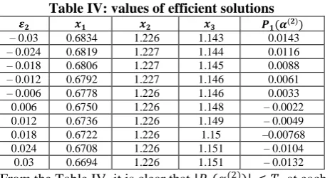
[image:5.595.321.532.48.131.2]Thus [𝜀2𝐿, 𝜀2𝑈] = [−2.01,1.37] and [−𝑇2, 𝑇2] ⊆ [𝜀2𝐿, 𝜀2𝑈]. So, we choose 𝜀2 ∈ [−𝑇2, 𝑇2]
Table IV: values of efficient solutions
𝜺𝟐 𝒙𝟏 𝒙𝟐 𝒙𝟑 𝑷𝟏(𝜶(𝟐))
– 0.03 0.6834 1.226 1.143 0.0143 – 0.024 0.6819 1.227 1.144 0.0116 – 0.018 0.6806 1.227 1.145 0.0088 – 0.012 0.6792 1.227 1.146 0.0061 – 0.006 0.6778 1.226 1.146 0.0033 0.006 0.6750 1.226 1.148 – 0.0022 0.012 0.6736 1.226 1.149 – 0.0049 0.018 0.6722 1.226 1.15 –0.00768 0.024 0.6708 1.226 1.151 – 0.0104 0.03 0.6694 1.226 1.151 – 0.0132
From the Table IV, it is clear that |𝑃1(𝛼(2))| < 𝑇1 at each efficient solution. Moreover, we can easily check that |𝑃2(𝛼(2))| ≤ 𝑇2 at each solution. Thus, Termination condition is satisfied by both 𝑃1(𝛼(2)) and 𝑃2(𝛼(2)). So, the
decision maker can choose any of the above find efficient solution as the best solution to the problem. The values of 𝑓1(𝑥) 𝑎𝑛𝑑 𝑓2(𝑥) which are evaluated at each above found
solution are :
Table V: values of objective functions
𝑥1 𝑥2 𝑥3 𝑓1(𝑥) 𝑓2(𝑥)
0.6834 1.226 1.143 0.4613 0.7304 0.6819 1.227 1.144 0.4603 0.73181 0.6806 1.227 1.145 0.3569 0.7328 0.6792 1.227 1.146 0.3567 0.7339
0.6778 1.226 1.146 0.3565 0.7340 0.6750 1.226 1.148 0.3561 0.7372 0.6736 1.226 1.149 0.3559 0.7372 0.6722 1.226 1.15 0.3557 0.7383 0.6708 1.226 1.151 0.3555 0.7394 0.6694 1.226 1.151 0.3551 0.7398
Comparative study of parametric method and fuzzy programming method:
Solution with the help of fuzzy goal programming is given by:
We know (𝑥11, 𝑥21, 𝑥31) = (0,1.281,1.31) and (𝑥12, 𝑥22, 𝑥32) = (1.13,0.619,1.05) are the individual optimal solutions of 𝑓1(𝑥) 𝑎𝑛𝑑 𝑓2(𝑥).
Also, (𝑓1)min = 0.2823 ≤ 𝑓1(𝑥) ≤ 1.065 = (𝑓1)max (𝑓2)min − 0.66 ≤ 𝑓2(𝑥) ≤ 1.511 = (𝑓2)max By solving the considered numerical example with fuzzy goal programming, best optimal solution comes out to be
(𝑓1(𝑥), 𝑓2(𝑥)) = (0.2842,0.9072)
Thus, we can see that the values of (𝑓1(𝑥), 𝑓2(𝑥)) calculated with the help of the proposed method and the fuzzy approach are comparable to each other and this validates the proposed method of parametric functions.
XI. CONCLUSION
This paper proposed an approach of solving MOQFPM by converting it into single objective non- fractional parametric programming Model with the help ofε-constraint method and this method can be extended for solving bi-level and multilevel fractional programming Models.The parametric approach used in the study makes it very easy to transform fractional objectives into non-fractional functions for which efficient solutions can be obtained easily. In the numerical example illustrated in the paper, the set of solutions obtained with the proposed method are comparable to those obtained with fuzzy approach, which validates the feasibility of our approach.
REFERENCES
1. Borza, M., Azmin Sham Rambely, and M. Saraj. ``Parametric approach for linear fractional programming with interval coefficients in the objective function." AIP Conference Proceedings. Vol. 1522. No. 1. AIP, 2013.
2. Emam, O. E. ``Interactive approach to bi-level integer multi-objective fractional programming problem." Applied Mathematics and Computation 223 (2013): 17-24.
3. Gupta1and, R., and M. C. Puri. "Extreme point quadratic fractional programming problem." Optimization 30.3 (1994): 205-214. 4. Heesterman, A. R. G. ``Parametric Methods In Quadratic
Programming." Matrices and Simplex Algorithms. Springer, Dordrecht, 1983. 516-555.
5. Hertog, Dick. Interior point approach to linear, quadratic and convex programming: algorithms and complexity. Springer, 1994.
6. Lachhwani, Kailash. ``On FGP Approach to Multiobjective Quadratic Fractional Programming Problem." International Journal of Applied and Computational Mathematics 3.4 (2017): 3443-3453.
7. Mishra, Savita, and Ajit Ghosh. "Interactive fuzzy programming approach to bi-level quadratic fractional programming problems." Annals of Operations Research143.1 (2006): 251-263.
8. Nayak, Suvasis, and Akshay Kumar Ojha. ``Solution approach to multi-objective linear fractional programming problem using parametric functions." OPSEARCH (2019): 1-17.
9. Nayak, Suvasis, and Akshay Ojha. ``Generating Pareto Optimal Solutions of Multi-Objective LFPP with Interval Coefficients Usingε -Constraint Method."
[image:5.595.55.287.495.620.2]oto
Author-3 Photo hor-1
10. Ojha, A. K., and K. K. Biswal. ``Multi-objective geometric programming problem with ε-constraint method." Applied mathematical modelling 38.2 (2014): 747-758.
11. Osman, M. S., O. E. Emam, and M. A. El Sayed. ``Multi-level Multi-objective Quadratic Fractional Programming Problem with Fuzzy Parameters: A FGP Approach." (2018).
12. Phillips, Andrew T. ``Quadratic fractional programming: Dinkelbach method." Encyclopedia of Optimization (2009): 3149-3153. 13. Salahi, Maziar, and Saeed Fallahi. ``Parametric approach for solving
quadratic fractional optimization with a linear and a quadratic constraint." Computational and Applied Mathematics35.2 (2016): 439-446.
14. Väliaho, Hannu. ``A unified approach to one-parametric general quadratic programming." Mathematical programming33.3 (1985): 318-338.
15. Zhong, Zhixia, and Fengqi You. ``Parametric algorithms for global optimization of mixed-integer fractional programming problems in process engineering." 2014 American Control Conference. IEEE, 2014.
AUTHORSPROFILE
Dr. Deepak Gupta is renowned personality working in the field of Operation Research. He is M.Sc., M. Phil., Ph.D. and working as a Professor & Head in the Department of Mathematics, Maharishi Markandeshwar Engineering College, Maharishi Markandeshwar (deemed to be University), Mullana, Ambala, Haryana, India. He is prolific author of over eighteen books of higher mathematics. He has had many statutory positions at Maharishi Markandeshwar University. He has to his credit more than two hundred research papers published in National/International Journal of repute. He has supervised eighteen candidates for Ph.D. and sixteen candidates for M. Phil. He has also written some books for under graduate students.
Dr. Suchet Kumar received his PhD in Mathematics at Guru Kashi University, Talwandi-Sabo (Bathinda), Punjab. He has cracked CSIR/UGC NET (June-2012) with AIR-18, GATE-2012 with AIR-52, Rajasthan State Eligibility Test-2012 for Lectureship and Haryana Teacher Eligibility Test-2016 for Post Graduate Teacher. Presently, he is working as teacher in Mathematics at Govt. Sen. Sec. School, Fatta Maloka (Mansa (PB)), India.