International Journal of Innovative Technology and Exploring Engineering (IJITEE) ISSN: 2278-3075,Volume-8 Issue-12, October 2019
Abstract: Forecasting paddy production is considered as a difficult problem in the real world due to in deterministic behavior of the nature. Specifically, rice production is forecasted for a leading year for overall planning of the crop, utilization of the agricultural resources and the rice production management. Likewise, the key challenge of the forecasting rice production is to create a realistic model that can able to handle the critical time series data and forecast with minor error. Prognostication of the Future data is highly correlated with the time series data set. If the accuracy of your prediction is more appropriate, then the value of the forecast will improve as well. This paper represents a new technique depends on Higher Order Fuzzy Logical Relationship. Here, Mean Square Error (MSE) and Mean Absolute Percentage Error (MAPE) are used to estimate the errors of predicted data. historical data relating to the rice production of 1981 to 2003 is used as secondary data and the error of the predicted data is further reduced using different soft computing technique.
Keywords: Fuzzy logical relationships, MSE, RMSE and Average Error.
I. INTRODUCTION
Time series forecasting is a crucial topic which deals with the various aspects of the future decision-making process in our everyday life. By set theory and linguistic variable presented by Zadeh [2, 3], Song and Chissom [1] developed the fuzzy time series concept. This is proficient of dealing with vague and imprecise data illustrated in terms of linguistic variables. Song and Chissom [4, 5] furthermore elongated this fuzzy time series theory to make it more efficient to deal with numerical data by adding the idea of fuzzification and defuzzification and applied it in the student enrollment forecasting program of Alabama university. Chen [6] analyzed the problem of large mathematical requirement of the Song and Chissom technique of calculating fuzzy relationships of max-min composition by replacing it with more simple arithmetic functions and applied this technique on the student enrollments of Alabama university. Different techniques of time series forecasting have been re-presented by Tsai and Wu [7], Huarng [8], Sullivan and Woodall [9]. Kim and Lee [10] developed a fuzzy time series
Revised Manuscript Received on September 05, 2019.
Surjeet Kumar* Engineering Technology and Management, University
of Kalyani, Kalyani, India. Email: [email protected].
Manas Kumar Sanyal, Engineering Technology and Management, University of Kalyani, Kalyani, India, Email: [email protected]
prognosticating technique on the basis of sequential values. Fuzzy time series forecasting is also structured as the time variant model by employing high-order techniques in fuzzy time series forecasting. Larger mathematical need is the main problem Song and Chissom [5] technique. To forecast the enrollments of upcoming years, the required numbers of past year’s the enrollments data were called the window basis The main purpose of this recent research work is to build a mathematical prediction model depends on the high-order (order 4 ) fuzzy logical relationship to reduce the average forecasting error of the existing fuzzy time series forecasting method and increases the accuracy of prediction value in agricultural production to help and support the farmers, producers or decision makers. The new approach is applied on the time series data of rice yield of Pantnagar farm G. B. Pant University of Agriculture and Technology, Pantnagar (INDIA). Rice crop production data has been enlisted with respect to quintal per hectare. This study comprises of a computational model construction and examining it on the rice yield production to verify its feasibility in forecasting over the other predictive techniques.
II. BASICSOFFUZZYTIMESERIES
Some fundamental concepts of the fuzzy time series models are summarized and is reproduced as [1,4,5].
Definition 2.1 A fuzzy set is a collection of entities with a continuation of grade of membership. Let ‘W’ be the Universe of discourse with W={ w1, w2, w3, …wn }, where Wi are viable semantic values of W, then a fuzzy set of semantic variables Xi of W is explained by Xi = μ Xi(w1)/( w1) + μ Xi(w2)/( w2) + μ Xi(w3)/( w3) +…….+ μ Xi(wn)/( wn) here, μ Xi is the membership function of the fuzzy set Xi , such that μ Xi : W→ [0,1]. If wj is the member of Xi, then μ Xi (wj) is the degree of belonging of wj to Xi (2).
II. I Prediction of Computational Procedures of Rice Yield Production
The execution of the given algorithm has been divided into four models: Chen’s arithmetic model (model-1), refined arithmetic model (model-2), Rajaram’s modified approach model (model-3) and a combined approach of Rajaram’s and Chen’s arithmetic model (model-4) for foretelling the rice production on the basis of time series data 1981 to 2003.
A Higher Order Fuzzy Logic Model with
Genetic Algorithm Used to Predict the Rice
Production in India
Process 1: The universe of discourse ‘W’ as [A min - A1, A max + A2] to accommodate the time series data, where A min and A max are the minimum and maximum historical production respectively. From table 1, we get A min = 3219 and A max = 4554. The variables A1 and A2 are just two positive numbers, properly chosen by the user. If we let A1 = 3219-19 = 3200 and A2 = 4554 + 46 = 4600, we get W = [3200-4600]. Process 2: Partition the universes of discourse into seven equal length intervals W1, W2, ,……..,W7 and each partition shows the range. W1 = [3200-3400], W2 = [3400-3600], W3 = [3600-3800], W4 = [3800-4000], W5 = [4000-4200], W6 = [4200-4400], W7 = [4400-4600].
Process 3: Define seven fuzzy sets X1, X2... X7 having some semantic values on the universe of discourse W. The semantic values to these fuzzy variables are as follows: X1: poor rice
production
X4: good rice production
X7: outstanding rice production X2: below avg rice
production
X5: very good rice production X3: avg rice
production
X6: excellent rice production
The membership grades to these fuzzy sets of linguistic variables are defined as -
X1= 1/w1 + 0.5/w2 + 0/w3 + 0/w4 + 0/w5 + 0/w6 + 0/w7 X2= 0.5/w1 + 1/w2 + 0.5/w3 + 0/w4 + 0/w5 + 0/w6 + 0/w7 X3= 0/w1 + 0.5/w2 + 1/w3 + 0.5/w4 + 0/w5 + 0/w6 + 0/w7 X4= 0/w1 + 0/w2 + 0.5/w3 + 1/w4 + 0.5/w5 + 0/w6 + 0/w7 X5= 0/w1 + 0/w2 + 0/w3 + 0.5/w4 + 1/w5 + 0.5/w6 + 0/w7 X6= 0/w1 + 0/w2 + 0/w3 + 0/w4 + 0.5/w5 + 1/w6 + 0.5/w7 X7= 0/w1 + 0/w2 + 0/w3 + 0/w4 + 0/w5 + 0.5/w6 + 1/w7 Process 4: Here, fuzzification helps to identify the relationships between the previous values in the dataset and define the fuzzy sets in the previous steps. Every previous value is fuzzified as stated by its highest degree of membership. If the highest degree of familiarity of a certain past time variable, says F(t-1), happens at fuzzy set Xk, then F (t-1) is fuzzified as Xk. In table 2, a general survey of fuzzification of the previous rice production data of different fuzzy time series models are shown. To give examples of this, year 1984 is fuzzified in model-1 and model-4. As table 1, rice yield of 1984 was 3455 (000’ tones) which lies within the boundaries of interval W2. Since the highest membership degree of W2 occurs at X2, the past time variable F (1984) is fuzzified as X2. The previous time series data [13] are fuzzified and are placed in table 1.
II. II The Actual and Fuzzified Data of Rice Production in Table. 1
Year Production Kg/
hect
Fuzzified production
Fuzzified Rang
Mid-point
1981 3552 X2 3400 – 3600 3500
1982 4177 X5 4000 – 4200 4100
1983 3372 X1 3200 – 3400 3300
1984 3455 X2 3400 – 3600 3500
1985 3702 X3 3600 – 3800 3700
1986 3670 X3 3600 – 3800 3700
1987 3865 X4 3800 – 4000 3900
1988 3592 X2 3400 – 3600 3500
1989 3222 X1 3200 – 3400 3300
1990 3750 X3 3600 – 3800 3700
1991 3851 X4 3800 – 4000 3900
1992 3231 X1 3200 – 3400 3300
1993 4170 X5 4000 – 4200 4100
1994 4554 X7 4400 – 4600 4500
1995 3872 X4 3800 – 4000 3900
1996 4439 X7 4400 – 4600 4500
1997 4266 X6 4200 – 4400 4300
1998 3219 X1 3200 – 3400 3300
1999 4305 X6 4200 – 4400 4300
2000 3928 X4 3800 – 4000 3900
2001 3978 X4 3800 – 4000 3900
2002 3870 X4 3800 – 4000 3900
2003 3727 X3 3600 – 3800 3700
II. III Higher Order Arrangement with Fuzzy Logical Relationship in Table. 2
1st order 2nd order 3rd order 4th order
X2→X5
X5→X1 X2, X5→X1
X1→X2 X5, X1→X2 X2, X5, X1→X2
X2→X3 X1, X2→X3 X5, X1, X2→X3 X2, X5, X1,
X2 → X3
X3→X3 X2, X3→X3 X1, X2, X3→X3 X5, X1, X2,
X3 → X3
X3→X4 X3, X3→X4 X2, X3, X3→X4 X1, X2, X3,
X3 → X4
X4→X2 X3, X4→X2 X3, X3, X4→X2 X2, X3, X3,
X4 → X2
X2→X1 X4, X2→X1 X3, X4, X2→X1 X3, X3, X4,
X2 → X1
X1→X3 X2, X1→X3 X4, X2, X1→X3 X3, X4, X2,
X1 → X3
X3→X4 X1, X3→X4 X2, X1, X3→X4 X4, X2, X1,
X3 → X4
X4→X1 X3, X4→X1 X1, X3, X4→X1 X2, X1, X3,
X4 → X1
X1→X5 X4, X1→X5 X3, X4, X1→X5 X1, X3, X4,
X1 → X5
X5→X7 X1, X5→X7 X4, X1, X5→X7 X3, X4, X1,
X5 → X7
X7→X4 X5, X7→X4 X1, X5, X7→X4 X4, X1, X5,
X7 → X4
X4→X7 X7, X4→X7 X5, X7, X4→X7 X1, X5, X7,
X4 → X7
X7→X6 X4, X7→X6 X7, X4, X7→X6 X5, X7, X4,
X7 → X6
X6→X1 X7, X6→X1 X4, X7, X6→X1 X7, X4, X7,
X6 → X1
X1→X6 X6, X1→X6 X7, X6, X1→X6 X4, X7, X6,
X1 → X6
X6→X4 X1, X6→X4 X6, X1, X6→X4 X7, X6, X1,
X6 → X4
X4→X4 X6, X4→X4 X1, X6, X4→X4 X6, X1, X6,
X4 → X4
X4→X4 X4, X4→X4 X6, X4, X4→X4 X1, X6, X4,
X4 → X4
X4→X3 X4, X4→X3 X4, X4, X4→X3 X6, X4, X4,
X4 → X3
II. IV Fuzzy Logical Relationship without Repetition in Table. 3
X2→ X5 X3 → X3 X1 → X3 X7 → X4 X1 → X6
X5 → X1 X3 → X4 X4 → X1 X4 → X7 X6 → X4
X1 → X2 X4 → X2 X1 → X5 X7 → X6 X4 → X4
X2 → X3 X2 → X1 X5 → X7 X6 → X1 X4 → X3
II. V Fuzzy Relationship Group in Table. 4
X1 → X2, X3, X5, X6 X5 → X1, X7
X2 → X1, X3, X5 X6 → X1, X4
X3 → X3, X4 X7 → X4, X6
X4 → X1, X2, X3, X4, X7
International Journal of Innovative Technology and Exploring Engineering (IJITEE) ISSN: 2278-3075,Volume-8 Issue-12, October 2019
II. VI The Available Data are Fuzzified Based on Gaussian Function Given in Table. 5
Actual value
X1 X2 X3 X4 X5 X6 X7
3552 0.24 1 0 0 0 0 0
4177 0 0 0 0.115 1 0.885 0
3372 1 0.86 0 0 0 0 0
3455 0.725 1 0.275 0 0 0 0
3702 0 0.49 1 0.51 0 0 0
3670 0 0.65 1 0.35 0 0 0
3865 0 0 0.675 1 0.325 0 0
3592 0.04 1 0.96 0 0 0 0
3222 1 0.89 0 0 0 0 0
3750 0 0.25 1 0.75 0 0 0
3851 0 0 0.745 1 0.255 0 0
3231 1 0.845 0 0 0 0 0
4170 0 0 0 0.15 1 0.85 0
4554 0 0 0 0 0 0.23 1
3872 0 0 0.64 1 0.36 0 0
4439 0 0 0 0 0 0.805 1
4266 0 0 0 0 0.67 1 0.33
3219 1 0.905 0 0 0 0 0
4305 0 0 0 0 0.475 1 0.525
3928 0 0 0.36 1 0.64 0 0
3978 0 0 0.11 1 0.89 0 0
3870 0 0 0.65 1 0.35 0 0
3727 0 0.365 1 0.635 0 0 0
III. BASICSOFGENETICALGORITHM Genetic Algorithm (GA) is a procedure for solving both constrained and unconstrained optimized problems which is based on natural selection. This Process is driven from Biological Evolution. At each step, the genetic algorithm randomly selects individuals from the current population (parents) and uses them to produce children of the next generation.
The three basic rules of GA are –
1.Selection - Select process is more important about the next generation, it’s totally depends on parents, which contribute to the population at the next generation. 2.Crossover – Randomly selects the pair of the bestsolution
(parents’ chromosome) and then interchanges to form a next generation.
3.Mutation – Depends on bit-wise probabilistic changing methods like 0 to 1 and vice versa.
Here, the Genetic Algorithm has been used to predict rice production data in India based on Fuzzy Logic Model. This rice production data set is a secondary data set. First, we predict data using first order fuzzification. Then the prediction accuracy is improved using Genetic Algorithm. Commonly, GA uses binary alphabet (0, 1) as notation. Hence, the data have to convert into binary form and that is called chromosomes. When the decimal to binary conversion happens, we manage the equality of bit for each data set. Chromosomes are represented into the decision variable domain. It helps to assess the performance, or fitness, of individual members of a population (9, 10).
In selection procedure, we have applied Roulette Wheel method. A fixed point is chosen on the wheel circumference and the wheel is rotated. The region of the wheel which comes in front of the fixed point is chosen as parent. For the second parent, the same process is repeated. It is clear that a fitter individual has a greater pie on the wheel and therefore a greater chance of landing in front of the fixed point when the wheel is rotated. Therefore, the probability of choosing an individual depends directly on its fitness.
In Crossover Method, after reproduction simple cross over may proceed in the steps. First, members of the newly reproduced strings in the mating pool are mated at random. Second, each pair of strings undergoes crossing over as follows: an integer with position k along the string is selected uniformly at random between 1 and string length less than one [1, l-1]. Two new strings are created by swapping all characters between positions k+1 and l inclusively. For example, two strings S1 and S2 are considered. Initial position, S1=0110101, S2=1100001. The resulting cross over yields two new string where the prime means the strings are part of new generations:
S1 = 0 1 1 0 0 0 1
S2 = 1 1 0 0 1 0 1
Mutation is a process of changing of the bit from 0 to 1 and vice versa with a small mutation probability pm. The bitwise mutation is performed as bit by bit by flipping a coin with the probability of pm.
Fitness Function: The fitness function must not only correlate closely with the designer's goal it must also be computed quickly. A fitness function is a particular type of objective function that is used to summarize, as a single figure of merit, how close a given design solution is to achieving the set aims. In this paper Mean Absolute Percentage Error (MAPE) is used as fitness function. The general equation of MAPE is as follow:
MAPE = 1/n ∑ [ (│Actual Value – Forecasted Value│) / Actual Value] * 100.
Where n is number of fitted point of data set.
IV. ERRORCALCULATIONTECHNIQUE
Accuracy of prediction error calculated in the basis of mean square error (MSE), root mean square error and average error.
1. Mean Square Error (MSE) = ∑ni=1(Actual Value(i) – Forecast Value(i))2 /n
2. Average Forecasting error = ∑ni=1[mod (Ei-Fi) / Ei] / n Where Ei =Actual value and Fi = forecast value
3. Residual Analysis –
Absolute Residual = mod [Actual value – Forecast value] Mean Absolute Residual = mod [Actual value – Forecast value]/Actual value.
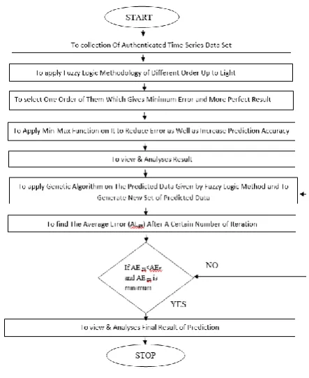
V. PROPOSEDMODEL
VI. RESULTANDDISCUSSION
[image:4.595.58.280.47.318.2]In this paper we have to use soft computing technique like fuzzy logic as an order wise. Fuzzified productions are selected as the midpoint from the universes of discourse depends on fuzzy logic of different order. The result then further fuzzified based on Gaussian function and produced ultimate result in the purposed model shown as table 6. Fourth ordered fuzzy logic gives optimized result and minimum error. Result accuracy of each order is better as compare to the using normal method of fuzzified.
Table 6. Actual data and higher order predicted data
We have to show that performance of accuracy at different order and proposed methods in the table below. Accuracy of predictions is calculated by using mean square error, root mean square error and average error.
Erro r calc ulat ion
1st order Prop osed meth od
2nd order
Prop osed meth od
3rd order
Prop osed meth od
4th order
Prop osed meth od
MS E
3092.5 9
3071 .60
2957 .524
2935 .55
2846 .2
2823 .127
2889 .42
2868 .52 RM
SE
55.61 55.4
2
54.3 83
54.1 80
53.3 49
53.1 33
53.7 4
53.5 5 Ave
rage Erro r
0.0133 0.01
329 0.01 309
0.01 305
0.01 268
0.01 263
0.01 242
0.01 29
Error calculation techniques are used in table 7. The rice productions juxtaposition of different fuzzy order, actual data, and proposed method are shown in graph 1. And graph 2. Shows the performance of accuracy and error calculation.
Graph 1. Accuracy of prediction is shows in different order
[image:4.595.48.292.458.770.2]International Journal of Innovative Technology and Exploring Engineering (IJITEE) ISSN: 2278-3075,Volume-8 Issue-12, October 2019
Table 8. Actual Data to Predicted Data Using Fuzzy Logic with Genetic Algorithm
Year Actual Data First Order
Fuzzy Logic Data
Proposed First order Data
Genetic Algorithm
1981 3552
1982 4177 4100 4100 4177.9
1983 3372 3300 3300 3372.8
1984 3455 3500 3499.27 3454.5
1985 3702 3700 3699.51 3702.1
1986 3670 3700 3699 3672.8
1987 3865 3900 3899.32 3864.8
1988 3592 3500 3500 3592.5
1989 3222 3300 3299.11 3222.2
1990 3750 3700 3700 3750.7
1991 3851 3900 3899.25 3852
1992 3231 3300 3300 3228.1
1993 4170 4100 4100 4170.7
1994 4554 4500 4500 4554.6
1995 3872 3900 3900 3873.1
1996 4439 4500 4500 4439.9
1997 4266 4300 4299.67 4266.1
1998 3219 3300 3300 3220.7
1999 4305 4300 4300 4306.8
2000 3928 3900 3900 3927.5
2001 3978 3900 3901 3978.3
2002 3870 3900 3901 3871.7
2003 3727 3700 3699.36 3727
Table 9. Accuracy of Prediction Error Comparison
Error Calculation MSE RMSE Average Error
First Order Fuzzy Logic
3092.59 55.61 0.0133
Modified Fuzzy Data
3071.60 55.42 0.01329
Genetic Algorithm 32.02 5.658 0.00502
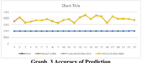
In the above table we have to show the only first order fuzzy logic with genetic algorithm comparison and get more accurate. In graph 3, show the accuracy of prediction. I have to applied same procedure in all the higher order and genetic algorithm always gives better accuracy.
Graph. 3 Accuracy of Prediction
VII. CONCLUSIONANDFUTURESCOPE In this study, time series data of rice production from 1981 to 2003 is used for prediction. Soft computing techniques like higher order Fuzzy logic are used to predict the simple and modified data set by using Gaussian function. Proposed methods are given more accurate prediction data for higher order compare to the general methods are used and I have also shown the individually accuracy of error using error calculation techniques in table 7. Further, we have to apply in genetic algorithm and get accuracy of prediction is more accurate as compare to the proposed fuzzy logic. Predicted data and error calculation shows in table 8, 9. In future, we will use different soft computing technique may give better
prediction accuracy at the same data set and also applying for different data set of crops and weather-related data.
REFERENCES
1. Q. Song and B. S. Chissom, “Fuzzy time series and its models”, Fuzzy
Sets and Systems, Volume- 54, page (269-277), 1993.
2. L. A. Zadeh, “Fuzzy Set, Information and Control”, Volume- 8, page
(338-353), 1965.
3. L. A. Zadeh, “The concept of a linguistic variable and its application to
approximate reasoning”, Information Sciences, Volume- 8, page (199–249), 1975.
4. Q. Song and B. S. Chissom, “Forecasting enrolments with fuzzy time
series”, Fuzzy Sets and Systems, Volume- 54, page (1-9), 1993.
5. Q. Song and B. S. Chissom, “Forecasting enrolments with fuzzy time
series”, Fuzzy Sets and Systems, Volume- 64, page (1-8), 1994.
6. S. M. Chen, “forecasting enrolments based on fuzzy time series”, Fuzzy
Sets and Systems, Volume- 8, page (311-319), 1996.
7. C. C. Tsai and S. J. Wu, “A study for second-order modelling of fuzzy
time series”, IEEE-1999.
8. S. M. Chen and J. R, “Hwang, Temperature prediction using fuzzy time
series”, IEEE Transactions on Systems, man, and Cybernetics, page (263-275), 2000.
9. K. Huarng, “Heuristic models of fuzzy time series for forecasting”, Fuzzy Sets and Systems, page (369-386), 2001.
10. J. Sullivan and W. H. Woodall, “A comparison of fuzzy forecasting and
Markov modelling”, Fuzzy Sets and Systems, Volume- 64, page (279- 293), 1994.
11. Kim and S.R. Lee, “A fuzzy time series prediction method based on consecutive values”, IEEE International Fuzzy Systems Conference, page (703-707), 1999.
12. Satyendra Nath Mandal, J Pal Choudhury and Dilip De, “Roll of
membership functions in fuzzy logic for prediction of shoot length of mustard plant based on residual analysis”, Journal World academy of science, engineering and technology, Volume- 38 pages (378-384), 2008.
13. Abhishekh Singh, “A Computational Method for Rice Production
Forecasting Based on High Order Fuzzy Time Series”, 2017.
AUTHORSPROFILE
Surjeet Kumar University Research Scholar (JRF), University of Kalyani West Bengal, Pursuing Ph.D (ETM), M.Tech (CSE), B.Tech (CSE).
[image:5.595.45.293.485.595.2]