Combining Testing and Proof to Gain High Assurance in Software: a Case Study

City, University of London Institutional Repository

Citation

: Bishop, P. G., Bloomfield, R. E. and Cyra, L. (2013). Combining Testing and

Proof to Gain High Assurance in Software: a Case Study. Paper presented at the IEEE

International Symposium on Software Reliability Engineering (ISSRE 2013), 4 - 7 Nov 2013,

Pasadena, CA, USA.

This is the unspecified version of the paper.

This version of the publication may differ from the final published

version.

Permanent repository link:

http://openaccess.city.ac.uk/2608/

Link to published version

:

Copyright and reuse:

City Research Online aims to make research

outputs of City, University of London available to a wider audience.

Copyright and Moral Rights remain with the author(s) and/or copyright

holders. URLs from City Research Online may be freely distributed and

linked to.

City Research Online:

http://openaccess.city.ac.uk/

[email protected]

Combining Testing and Proof to Gain High

Assurance in Software: a Case Study

Peter Bishop, Robin Bloomfield

London, UK {pgb,reb}@csr.city.ac.uk

{pgb,reb}@adelard.com

Lukasz Cyra

European Commission - Joint Research Centre Institute for the Protection & Security of the Citizen

Ispra, Italy

[email protected]

Abstract— Dynamic software test methods are generally easy to use, but the results only apply to the specific input values tested. Static analysis produces results which are more general, but can require more effort to perform. There are potential benefits in combining both types of techniques because the results obtained can be more general than standalone dynamic testing but less resource-intensive than standalone static analysis. This paper presents a specific example of this approach applied to the verification of continuous monotonic functions. This approach combines a monotonicity analysis with a defined set of tests to demonstrate the accuracy of a software function over its entire input range. Unlike “standalone” dynamic methods, our approach provides full coverage, and guarantees a maximal error. We present a case study of the application of our approach to the analysis and testing of the software-implemented transfer function in a smart sensor. This demonstrated that relatively low levels of effort were needed to apply the approach. We conclude by discussing future developments of this approach.

Keywords— test strategies, dynamic analysis, static analysis, formal proof

I. INTRODUCTION

Software systems can be analysed using both static and dynamic methods. Dynamic tests are easy to implement but only demonstrate correctness at specific inputs, while static analysis can be resource-intensive but the results can apply to all the possible inputs. There are potential benefits in combining both types of techniques because the results obtained can be more general than standalone dynamic testing but less resource-intensive than standalone static analysis.

In this paper we present a specific combination of static and dynamic analysis techniques that can be used to verify the accuracy of software which implements monotonic functions. Continuous monotonic functions are often implemented in the software of real-time embedded systems (e.g. when sensor measurements are converted into process state values) so the approach described in this paper can be applied to actual industrial systems. We describe how to guarantee the maximal error of the software over the entire input space using a combination of static analysis and systematic tests. We also show that application of our method requires much less effort than full formal analysis and far fewer test cases than extensive testing. The technique was developed as part of continuing

research funded by the UK nuclear industry that is developing methods for assessing the behaviour of commercial off the shelf smart devices.

In Sections II and III we discuss static and dynamic techniques, and methods of their combination. Section IV presents our approach to analysing monotonic functions. Section V generalises the approach to functions of multiple variables. Section VI gives examples of applicability of the approach. In Section VII we discuss the level of support provided by the available tools. In Section VIII we present a case study of application of the method. Finally, we conclude and discuss our future plans in Sections IX and X.

II. STATIC AND DYNAMIC ANALYSIS

Static analysis is the analysis of computer software which does not require execution of the software. It is commonly considered that the use of static analysis to verify program correctness requires specialist expertise and considerable computational resources but provides sound (though possibly conservative) results. However, there are more limited forms of static analysis that are widely used, e.g. all the compilers are

static code analysers, many software development

environments have tools to compute certain code metrics (e.g. cyclomatic complexity) and check simple soundness properties (such as type checking, data flow analysis or control flow analysis).

Static methods of software verification are very often applied in development of safety and security related systems, systems with high reliability requirements and in development of hardware [1]. To this end, methods are provided for specifying properties of systems formally, which are then demonstrated by analysis of the code using a formal proof tool [2]. Another approach is to analyse abstract models of systems and infer properties of the systems from the models (e.g., using model checking) [3]. Some inferences can be fully automatic (e.g. using model checkers or code analysis tools based on automatic Satisfiability Modulo Theories (SMT) solvers like SAL and SMV). For more complex problems, the analysis requires manual intervention and guidance (e.g., using proof tools like PVS and HOL).

Dynamic analysis techniques, by contrast, depend on analysis of the behaviour of programs through their execution

and are routinely used in software development. Correct functionality cannot usually be demonstrated over the entire input space, but only at selected test points in the input space (e.g. chosen to achieve full code coverage) [4]. However, they can be applied to complex systems and they are supported by mature, industrial quality tools. Dynamic analysis techniques are also supported by tools for test coverage estimation (like LDRA Testbed and Cantata++). Dynamic techniques also provide confidence in the tool chain between the code analysed with static techniques and the actual executed firmware.

Although, static and dynamic analyses differ significantly, combination of both approaches is tempting. It offers the prospect of more effective forms of verification, either by reducing test effort, or by increasing the coverage achieved by the tests.

III. METHODS OF COMBINATION

Efforts to combine static and dynamic analysis are being made by two different communities, i.e. hardware and software developers. Currently, there are only a limited number of combination strategies and it is recognised that further research is needed [1] to realise the full potential.

Currently, several approaches and tools exist, which take advantage of these ideas. Depending on the level of integration the advantages can differ. To present the differences we distinguished four levels of combination.

In the most basic form of integration developers decide which parts of the system should be analysed using either static or dynamic approaches. Both approaches have different advantages and disadvantages and they suit different problems. Therefore, in large systems development, static and dynamic methods can be applied together in an ad-hoc way to support each other or to analyse different parts of the same system. There even exist solutions which make mutual application of both approaches easy. JNuke [5], for instance, provides an interface for writing the analysis logic regardless of the type of analysis, and defines a framework in which dynamic analysis can be used to confirm the findings of static analysis.

At the next level of integration, static analysis can be used to support dynamic analysis of systems; or vice versa. Static analysis can help define comprehensive test suites, or it can be used to increase efficiency of testing, like:

• Conformance testing – this is a commonly used

approach (especially to test telecommunication

protocols implementation) to demonstrate conformity of protocols with their specifications [6]. Appropriate test cases are derived automatically from a formal model of the protocol and then are used to test the protocol implementation.

• Automatic test case generation – different approaches

to automatic test case generation exist, which provide for definition of test case suites with certain properties (e.g. path coverage) [8] [9] [10] [11].

Detection efficiency during testing can also be improved by formally defined run-time checks including:

• Assertions – these are commonly used to provide for

more efficient testing, and increase the coverage of testing [7]. Assertions are manually specified by developers in the code and then they are dynamically verified during execution. Assertions can also be used to specify properties of interfaces of different modules so that interface consistency can be checked during integration.

• Automatic invariants/assertions discovery – there exists

a set of approaches [12] [13] [14] [15] which provide methods for monitoring the application during execution in order to discover possible code invariants. This information is then used at the stage of selecting objectives for the static analysis.

At the third level of integration we can use static analysis not only to plan testing but also to analyse the results. Test results of the system are combined with static analysis results of modules of the system and then the analysis coverage is estimated by performing static analysis of the code. The ‘0-In Formal Verification’ method [17] is an example of this level of integration.

Finally at the fourth level, static and dynamic methods can be fully combined. A precisely selected set of tests are identified and the test results are enhanced by formal analysis to demonstrate that some property holds for the whole domain of possible inputs, see, for example [16]. More formally, we can regard a program f(⋅) as an implementation of a specification f′(⋅) that performs a mapping between an input domain I and an output range O. The combination of static and dynamic analysis comprises:

• a formal proof of some property P of program f(⋅)

• a specific set of test inputs T drawn from the input domain I that meet some success criterion C between the test input and the result.

This combination of test and proof is designed to show that some behavioural predicate B of the function f(⋅) is true over the whole input domain I, i.e.

)) ( , ( ))

( ), ( , ( ))

( (

, C t f t f t B i f i f

P

I i I

T T

t∈∀⊂ ′ ⇒∀∈

∧

⋅ (1)

The method presented in this paper belongs to this fourth group and we think it is an innovative example of this integrated approach. In this specific example, the behavioural property B we need to demonstrate is accuracy, i.e. that the implemented program f(⋅) meets some maximal error bound relative to the specification f′(⋅). This is achieved by combining a proof of monotonicity with a carefully selected set of tests.

IV. COMPOSITE VERIFICATION TECHNIQUE FOR

MONOTONIC FUNCTIONS

knowledge of the implementation, we cannot interpolate the response between test points as software behaviour might be discontinuous. To generalise test results to cover the whole input domain, we use a combined verification approach.

Firstly, we must show that the function implemented in the firmware is monotonic. A monotonic function is a function

f(⋅)which takes its input from I and fulfils either condition (2) or (3) below.

) ( ) (

,y Ix y f x f y

x ≥

⇒

≥

∀_∈ (2)

) ( ) (

,y Ix y f x f y

x ≤

⇒

≥

∀_∈ (3)

Secondly, we select test points using the specification of the function f′(⋅) and the desired maximal error guarantee. If testing confirms proper implementation of the function for the selected inputs we can deduce that the maximal error of the implementation for any other input is not greater then the desired maximal error guarantee. If we relate this to the formal definition of composite verification given earlier, the predicate P(f(⋅)) is monotonicity as defined in (2) or (3), the success criterion C is f′(t)=f(t) for all tests t and the behaviour predicate B is │f′(x)-f(x)│≤maxfor all input values x.

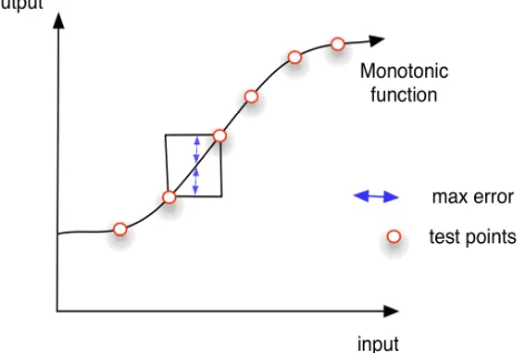
A graphical illustration of the composite verification method is given in Fig. 1. The points on the curve represent test points, where the correctness of the implemented function is checked. If we know that the implemented function is monotonic increasing (which is demonstrated formally by static analysis or manually by inspection of the code) then the values of the implemented function for inputs between two adjacent test points is bounded by the values of the function in the test points. It follows that the graph of the implemented function at intermediate points must be within the rectangle shown in Fig. 1.

Fig. 1. Composite verification technique for monotonic functions

The maximal error cannot exceed the absolute difference between the values in the two test points and for the whole

function the maximal error of implementation cannot exceed the maximal absolute difference between the values of the function in two adjacent test points.

More formally, if we assume that we have tested function

f(⋅) in two points: x and y and we have demonstrated formally that the function is increasing monotonically, then for any point between x and y, the value of the function has to be between

f(x) and f(y). Therefore, the maximal error of the

implementation of the function cannot exceed | f(x)− f(y)| for any of the inputs between x and y.

For example, let us take function f(x) = x + 1 which takes as input a value from the range <0, 5>. Implementation of the function in C is presented in Fig. 2.

int f(int x) { return x+1; }

Fig. 2. Implementation of a linear function

We can easily prove monotonicity of this function. We can do this by writing a specification of this code in a formal language and using a static analyser to prove it automatically; or we can do it manually.

Examples of code specifications and discussion of their automatic verification are presented in the following sections. Equation (4) contains a manual proof of monotonicity of this function.

) ( ) (

1 1

y f x f

y x

y x

≥

=> + ≥ +

=> ≥

(4)

Now, let us assume that we have tested the implementation of the function for 6 inputs: 0, 1, 2, 3, 4, and 5; and that the outputs were correct.

As the difference between the values of two adjacent test inputs is not greater than 1 for any pair, the composite verification technique provides us immediately with the information that the maximal implementation error of

f(x) = x + 1 for any input from the range <0, 5>is not greater than 1.

We would not be able to obtain the same result using dynamic analysis (even if we tested the implementation for thousands of inputs). We would be able to prove correctness of the implementation statically (but using proof alone does not give us confidence in the implementation within the firmware); however, for more sophisticated functions such a proof would be much more difficult than a proof of monotonicity.

A. Assumptions

This method can be applied when the following assumptions hold:

• We know the specification of the function f′. • The specified function is monotonic.

• We are able to test the implementation of the function f, and conclude whether the response for a given input is correct or not.

B. Analysis of Monotonicity

In comparison to proving correctness, demonstration of monotonicity of a function implementation f is a fairly easy task.

For most of the software it can be done manually, while still giving high level of assurance. To this end we can analyse the software functions implementing the transfer function in isolation, proving monotonicity of each of them separately. Then from the superposition of monotonic functions we can deduce monotonicity of the end-to-end program function.

Alternatively, if we aim at a very high level of confidence, we can provide a formal proof of monotonicity, whose correctness is automatically verified by static analysis tools. The principle idea of the proof is the same as for the manual approach. Formal demonstration of monotonicity in theory is a relatively easy task, i.e. it is much easier than formal demonstration of correctness of implementation. In particular, to specify correctness, we would require a complete and correct formal specification for each program function, which can be difficult to construct and certify. By contrast the specification of monotonicity is easy to specify and is the same for all functions. We, however, encountered certain difficulties in practical implementation of this idea caused by missing functionality in the static analysis tools available on the market (see Section VI).

C. Testing

The next step of the method is to define a test schedule, which specifies test input values that are sufficient to demonstrate a particular maximal error. These tests rely on the existence of an independent “reference function” f′ that can be used to derive independent test cases for the implemented function. Different test generation options that satisfy the maximal error condition are described below.

Function-based approach. If test inputs are evenly spaced

across the input range, it can be shown that if r is the required accuracy (expressed as a proportion of full-scale), you need 1 + (1/r)(amax/amean) test points, where amax is the maximum

slope of the continuous function on the range considered, and

amean is the average slope of the function on the range

considered. The maximum and mean slopes are derived from the specified function f_′. For example for 1% accuracy, where the maximum slope of the transfer function was twice the average slope, we would need 201 test points evenly spaced over the smart sensor input range.

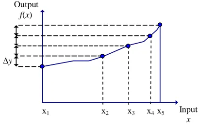
Inverse function. The test values are defined by x= f′−1(y) where f′−1 is the inverse of the specified function y=f(x) and the output values y are evenly spread over the output range. It can be shown that the minimum number of tests needed for a given accuracy r is 1+1/r. For example for 25% output accuracy, the minimum number of tests is 5. To compute the test values, the output range is evenly split by 5 output values and the equivalent test input values are calculated by inverting the specified transfer function f′). This approach is illustrated in Fig. 3. The interval Δy is the maximal error (r times full-scale)

and x1… x5 are the derived test points.

Input

x

∆y

x1 x2 x3 x4

Output

f(x)

x5

Fig. 3. Defining test points – inverse function

V. GENERALISATION TO FUNCTIONS OF MULTIPLE VARIABLES

The composite verification technique for monotonic continuous functions can be generalised to functions of multiple variables. This is an important issue as functions of this type are commonly used in firmware of smart sensors, e.g. as averaging filters to process the input values.

For functions of multiple variables the monotonicity analysis must prove that the functions are monotonic in respect to each of the variables.

Let us consider function f(p1,…,pn) of n parameters. The monotonicity analysis must prove that each of the functions

f1(),…,fn() defined in (5), where x1,…,xn can be any point from the input ranges, is monotonic.

) , ,..., ( ) ( ...

) ,..., , ( ) (

1 1

2 1

z x x f z f

x x z f z f

n n

n

−

= =

(5)

Proving monotonicity for an n parameter function will be more time-consuming, but the proofs of monotonicity share a lot of content, making the formal analysis easier to repeat.

i i i p f R R a ∂ • ∂ =max '( )

*max (6)

The normalised spacing ri (∆xi/Ri) for the grid of test points along input axis i depends on the worst case gradient on that axis ai*max and the required maximal normalised error r. When the grid spacing on each axis makes a maximal error contribution r/n, the normalised grid spacing on each axis i is:

max

*

a

n

r

r

⋅

≤

With this n-dimensional test grid, the required number of test points, ntest is:













⋅

_

+



∏

=

r

a

n

n

*

1

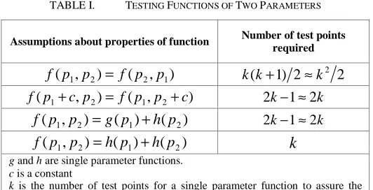
So if k tests are needed for a single parameter function we need ≈ (nk)n tests for n parameters, however, tests may be reduced if we take account of the specific properties of the function. Table 1 below gives examples of additional properties of commonly used two parameter functions that reduce the required number of test points.

TABLE I. TESTING FUNCTIONS OF TWO PARAMETERS

Assumptions about properties of function Number of test points required

)

,

(

)

,

(

p

p

f

p

p

f

=

, ( ) ,

(p₁ c p₂ f p₁ p₂ c

f + = + 2k−1≈2k

)

(

)

(

)

,

(

p

p

g

p

h

p

f

=

+

)

(

)

(

)

,

(

p

p

h

p

h

p

f

=

+

k

g and h are single parameter functions. c is a constant

k is the number of test points for a single parameter function to assure the maximal error is not greater than r

An example proof of this test reduction is given for the following function (which might typically be used for averaging successive input signals).

) ( ) ( ) ,

(p1 p2 h p1 h p2

f = + (9)

Equation (10) shows that the output of the function for any test point can be derived from the outputs for (x1,x1),…,(xk,xk).

) , ( ) , ( )) ( ) ( ( )) ( ) ( ( ) ( ) ( ) , ( 2 1 2 1 2 1 2 1 j j i i j j i i j i j i x x f x x f x h x h x h x h x h x h x x f + = + + + = + = (10)

Therefore, if k tests are sufficient for testing function h, k tests are also sufficient to test function f. Clearly the same result would apply to an arbitrary number of parameters for a function of this type.

VI. FORMAL DEMONSTRATION OF MONOTONICITY

Traditionally static analysis tools model software as machines with operations and state variables, with certain invariants and initialisation parameters. The definition of an operation, according to this viewpoint, is defined as a tuple composed of [18]:

• a name

• input parameters

• output parameters

• restrictions on parameters and the states from which the operation may be called

• variables that may be modified

• the effects or behaviour of the operation

This strict state-based approach is well suited to program specifications and can successfully be applied to a wide range of problems. Industrial implementations of this approach exist for analysis of program logic, concurrency, timing, mobility, security, etc.

While this approach is powerful, there are limitations to a strict state-based approach. To specify some properties of a function we have to compare two invocations of the same function, e.g. for non-interference analysis [19]. The same requirement exists when specifying monotonicity—we would like to specify the property directly as shown in equations (2) and (3). Unfortunately ACSL (the ANSI/ISO C Specification Language which defines the syntax for writing specifications for programs in C) [20] does not support specifications of this type.

After reviewing around twenty possible code analysis tools, we decided to use Frama-C [21], which fulfilled all our requirements (apart from the specifications involving the comparison of function calls). Frama-C is a tool which is being actively developed by Commissariat a l’Energie Atomique and INRIA. Frama-C has a range of plug-ins that can perform a variety of analyses including

• code safety checking including pointers dereferencing and divisions by zero

• observation of possible values of the application variables at each point of execution

• slicing the original program into simplified ones

• proving formal specifications of particular C functions or the whole application

• integration with the most popular automatic theorem provers and proof assistants

ACSL. ACSL provides good support for expressing relationships between functions’ input and output, provides for specifying functions entry conditions, and supports formal specifications of data structures.

As we have already mentioned Frama-C did not meet all our requirements. To be able to apply it successfully we had to find a work-around for the tool limitations. To specify monotonicity, we had to add extra code to the program, which invokes the function twice and compares the results. By adding this extra code we were able to specify monotonicity not as a property of a function (dependant on its two invocations) but as a property of the input and output values of the new function we added to the code. For example, to specify monotonicity of function f(x) we add another function monotonicity_check(x,y) that compares the result of two invocations of f(x) with ACSL annotations that specify the expected result of the comparison if f(x) is monotonic (see Fig. 4 below).

// the function of interest

int f(int x) { // body of f() }

/*@ behaviour monotonicity: @ ensures x > y ==> \result == 1; @*/

int monotonicity_check(int x, int y) { return f(x) >= f(y) ? 1 : 0;

}

Fig. 4. Monotonicity specification

The comment lines with a “@” prefix are ACSL specification statements.

VII. CASE STUDY

This section contains the description of a case study, in which we applied our method of monotonicity analysis using the composite verification approach to a real-world device used in the nuclear industry.

A. Objectives

For the case study we selected a commercially available smart sensor device from a number of instruments that we have been assessing for deployment on nuclear power plants. This smart sensor was a programmable alarm unit that can measure plant parameters, transmit the measured value and raise an alarm if a programmable limit is violated.

The alarm unit smart sensor considered in this study can monitor a wide range of plant parameters; for instance temperature, pressure, flow, position, etc. and can handle anything from simple annunciation to shut down of an entire process. The device can handle up to four relay outputs. The relays can control such devices as warning lights, bells, pumps, motors, shut down systems, and so on.

The smart sensor can be configured to:

• read in different types of plant input signal

• transmit the converted plant value in different formats

• raise an alarm on high or low measured values

• raise an alarm if internal errors are detected.

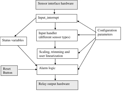
The smart sensor software comprises around 12 000 lines of C source code (excluding blank lines and comments). It is written in a generic way and is used on several models of the device. Analysis of the software shows that the data processing is implemented using a sequence of functions as shown in Fig 5.

Input_interrupt

Input handler (different sensor types)

Scaling, trimming and user linearization

Alarm logic

Sensor interface hardware

Relay output hardware Status variables

Configuration parameters

Reset Button

Fig. 5. Processing functions and data flows

The blocks in the diagram are described in more detail below.

Sensor interface hardware – is a piece of hardware that

receives input and makes it available to the software

Status variables – are variables set by hardware which

among other things provide information about the device failure

Reset button – is a button on the device which when

pressed resets the alarm if the device is working in a “latching” mode

Configuration parameters – are values in memory which

store information about the model of device and mode of operation of the alarm, e.g. “high-trip”, “low-trip”, “latching”, etc.

Relay output hardware – is a piece of hardware which

transforms a decision of the firmware whether to set an alarm or not into an electric signal

Input_interrupt – is an interrupt function called whenever

there are new readings available. It reads the device registers, and copies the values to a selected memory location

Input handler – is a very complex function (over 1000 lines

Scaling, trimming and linearization – are three functions

performing transformation of the input signal according to the device configuration

Alarm logic – is a set of functions implementing the alarm

logic, which based on the value of the transformed input decide whether to set the alarm or not.

The objective of the study was to demonstrate that the maximal error of the software implementation of data processing of the sensor in a given configuration is no more than 1% of the input range. To this end we decided to perform a static analysis to show monotonicity of the transfer function, and to define and perform tests assuring satisfaction of the analysis objective in the given configuration.

B. Monotonicity Argument

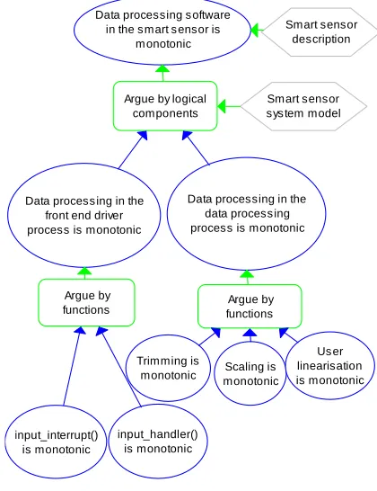
To demonstrate that the smart sensor firmware provides an output conversion that is monotonic with respect to its input, a safety argument [23] was constructed to identify which pieces of the code must be demonstrated to be monotonic (see Fig. 6).

Scaling is monotonic Trimming is

monotonic

Data processing in the data process ing process is monotonic

Us er linearisation is monotonic Argue by

functions

input_handler() is monotonic input_interrupt()

is monotonic Argue by functions Data process ing in the

front end driver process is monotonic

Argue by logical components Data processing s oftware

in the s mart s ensor is m onotonic

Smart sensor description

Smart sensor sys tem model

Fig. 6. Monotonicity argument

To demonstrate that the data processing software in the smart sensor is monotonic, we have to consider two stages of data processing, which correspond to two parts of the argument:

• The data input – which is responsible for conversion of the input signals into normalised form. This is implemented by input_interrupt() and input_handler() which must be demonstrated to be monotonic.

• Subsequent data conversion – this is implemented by functions: trimming(), scaling() and linearisevalue() which must also be demonstrated to be monotonic

C. Analysis Approach

To demonstrate monotonicity of the code we had to use the workaround for the tool limitations identified in Section VII. This, however, had significant impact on the analysis and difficulty of this task.

First and foremost, the workaround makes it possible to demonstrate monotonicity of a function by defining an additional one, whose properties are equivalent to the claim we want to prove (see Section VI for details). While this approach is valid, it makes reuse of the specification impossible. For example in Fig 7, we are not able to infer properties of f(⋅) using a superposition g(⋅) and h(⋅) properties.

int f(int x) { return g(x) + h(x) }

Fig. 7. Superposition of functions

If we were to use a tool which supports monotonicity analysis, we would be able to specify and prove monotonicity of g(⋅) and h(⋅). Then, very easily we would prove monotonicity of f(⋅), referring to the specifications of g(⋅) and h(⋅). However, because of the limitations of the available tools, we are not able to specify that g(⋅) and h(⋅) are monotonic in a way that can be utilised to demonstrate monotonicity of f(⋅). To be able to reach any conclusions we had to use one of the following strategies:

• partly switch to manual proofs,

• specify the functions implemented by g(⋅) and h(⋅) (which is a much more resource intensive task). In our case study we made use of both of the solutions.

In the smart sensor case study:

• We demonstrated manually that monotonicity of each of the functions identified in Subsection B implies monotonicity of the whole transfer function of the device.

• We analysed each of the functions in isolation.

The proofs we performed are summarised in the following sections.

D. Front-end Driver Functions

Input_interrupt() is a simple function and its monotonicity

was demonstrated formally in Frama-C.

Creating a complete formal proof for input_handler(), on the other hand, was not possible due to complexity of the function (over 1000 lines of code) and lack of resources. Therefore, the following approach was applied:

• Assumptions about the device type were written in the form of ACSL assumptions (using the “ensure” keyword).

• Monotonicity of certain intermediate variables derived by the function was formally demonstrated.

• Manual proofs for the monotonicity of all the sub-functions invoked by input_handler() was provided.

• A manual proof was created to show that the rest of the function applies monotonic transformations on the process variables.

E. Data Processing Functions

To demonstrate monotonicity of trimming() and scaling() we applied the following process:

• Certain assumptions were made about values of global variables, when trimming() and scaling() are invoked. We assumed that certain configuration variables contain certain values, e.g. that trimming and scaling is on. We also assumed that certain function parameters are in certain relations, e.g. that the upper bound value is greater than the lower bound value in the definition of the scaling parameters.

• An additional function was added to the code in order to make monotonicity specification feasible (see Fig. 8).

/*@ requires @ x > y &&

@ SCALING_ENABLED && @ TRIMMING_ENABLED &&

@ SC_UPPER_BOUND > SC_LOWER_BOUND && @ TR_UPPER_BOUND > TR_LOWER_BOUND @ ensures

@ \result >= 0.0; @*/

float scaling_monotonicity(float x, float y) { PV = x;

Trimming(); Scaling();

float rx = PV_Scaled; PV = y;

Trimming(); Scaling();

float ry = PV_Scaled; return rx - ry;

Fig. 8. Trimming() and scaling() monotonicity specification

• The code was annotated in a way which expresses the properties to be demonstrated.

• Assertions and lemmas required to complete the proof were added. This step was necessary, because to demonstrate compliance of the code with the specification we used automatic theorem provers. Automatic provers are quite powerful, however, they are not ideal and sometimes require some help to be able to do their work. In particular, we had to specify some invariants of the key variables in the code. We also had to add some lemmas relating to basic mathematical theorems, as automatic theorem provers do not support calculations on floating point variables very well. Fig. 9 is an example of such a lemma.

/*@ lemma multiplication: \forall float x,y,z; (x > y && z >= 0.0) ==> x*z >= y*z; */

Fig. 9. Lemma example

• Monotonicity of superposition of the two functions was specified formally. We demonstrated formally all the monotonicity specifications. We executed Frama-C, which generated a set of verification conditions. All the verification conditions (apart from the lemmas) were demonstrated formally by using one of the Frama-C automated theorem provers (alt ergo 0.8). A screenshot of the results of proving monotonicity of trimming() and

scaling() is shown in Fig. 10.

•

Fig. 10.Frama-C analysis results

The red triangles indicate that the lemmas are unverified. The green ticks indicate that all the verification conditions for the functions have been satisfied. This demonstrates that superposition of the two functions is monotonic, given that the lemmas are correct. It states that multiplication of both sides of an inequality by a non-negative value preserves this relationship.

Due to limitations of Frama-C and lack of resources for complete formal verification of the code the linearisation function was demonstrated to be monotonic manually.

F. Testing

tests on the code. Test execution was implemented in the form of integration tests and executed automatically using the CUnit framework. This step completed our analysis, which demonstrated that the firmware of the smart sensor provides output within a 1% error band, i.e. that the alarms are guaranteed to work given the input value exceeds the limit by more than 1% of the input range.

G. Analysis Effort

The static analysis took 15 days to perform, which seems to be a reasonable expenditure considering the extra confidence that was gained from the quite limited testing. The effort required to perform the analysis was hampered by lack of off-the-shelf tools that could directly perform a monotonicity analysis. Otherwise, we could have obtained the same results in a significantly shorter time. We estimate that manual static analysis could have been undertaken in 2 days (but with a lower confidence that the analysis is correct).

The effort required to perform the testing was only one day. Since the tests were automated, it would have been feasible to test at much finer resolutions (e.g. 0.1%) in a similar amount of time.

VIII. DISCUSSION

The use of proof applied to the actual code to demonstrate a behavioral property is not a common approach. Typically, static analysis is used to automate test case generation from either the code, a formal specification or a formal behavioural model.

There are some examples that are similar to our approach where the code is subjected to static analysis to prove some property or invariant. For example in [24] a simplified approximation function in a navigation system is proved to guarantee some maximum level of error in a trajectory. This is similar to our own approach where the invariant we seek to demonstrate is the maximal error. The main difference, is that our approach combines testing at selected points with a relatively weak code property (monotonicity) to demonstrate the required invariant (maximal error)

Our method can be successfully applied to situations which require high confidence in a given level of accuracy (e.g. the level necessary to guarantee safety rather than optimal performance). This means that the approach is well suited to cases where software is used to process values from analogue inputs or values sent to analogue outputs (such as the smart sensor software used in our case study). We can always select a set of test points to guarantee the maximal error to be significantly lower than the accuracy level of the analogue hardware of the device.

The approach to the problem we presented in this paper is based on formal analysis and formal verification tools. The formal verification tools available did not directly support this type of analysis, which impeded the monotonicity analysis. Nonetheless, this analysis was still easier to perform than a complete proof of correctness.

There is, however, an alternative. We could have performed the whole analysis manually by inspecting the

conversion equations within the software (which could be assisted by code slicing tools). This would be much easier to perform than a formal analysis (e.g. probably only two days of effort to manually assess the monotonicity of the conversion functions within the smart sensor software would be needed). This alternative form of analysis would still provide high level of confidence in the correctness of the results as the monotonicity of a function is relatively easy to determine by code inspection.

The approach to analysing monotonic functions’

implementations has been generalised to functions of multiple variables, which is presented in Section V. This provides a whole set of new applications. The number of tests required remains reasonable and for many types of functions is the same as for functions of single variables.

Apart from the method presented in this paper we have also been considering enhancements to our approach. For instance:

We could divide the input range into sub-ranges and consider them in isolation. This in certain situations may be much easier, as definitions of software functions over the whole input domain tend to be very complex. Division of the range into sub-ranges may reduce the number of parameters considered in each proof step. In this case, however, apart from proving monotonicity of the function on each of the ranges we would also need to provide a proof of monotonicity of the function on combination of the sub-ranges, i.e. to show that monotonicity on the endpoints is preserved and that the type of monotonicity on each of the sub-ranges is identical (where the sub-range functions are either all increasing or all decreasing).

For the special case where the function is linear, the number of tests can be reduced even further. Provided that the formal analysis can demonstrate linearity, it is only necessary to test the two end points.

More generally, the use of static analysis to generalise some property from individual test points to a whole domain can have much wider application.

For instance, in nuclear applications, another property important to safety is that a trip relay will actuate when the linearised value reaches a trip limit, i.e.:

trip x

f I x

⇒

>

∀_∈, ( ) lim (11)

So if the relatively short section of trip logic code is formally proved to satisfy the trip property in (11), this can be combined with maximal error property, namely that

│f′(x)−f(x)│≤ max to show that:

trip x

f I x

⇒

+ > ′

∀_∈ ( ) lim max (12)

This safety-related property specifies the trip behaviour relative to the actual state of the process over the whole input range.

could be verified using a combination of dynamic and static analysis. This need not be limited to purely functional properties as the approach can also be applied to non-functional properties like worst case timing [16].

IX. CONCLUSIONS

In this paper we presented a verification approach based on a combination of testing and static analysis—the verification of the accuracy of monotonic functions. We described the theory which lies behind the approach and presented a case study of successful monotonicity analysis of a smart sensor used in the nuclear industry. We conclude that:

• A verification technique that combines monotonicity analysis with testing at selected inputs has been successfully demonstrated on an industrial software example.

• The approach enables test results made at selected test points to be generalised to a claim about the accuracy of the software over the whole input space.

• The approach is more rigorous than testing alone, but less expensive than full formal proof and could be an efficient technique for enhancing confidence in software with finite accuracy requirements.

• The monotonicity analysis effort could be reduced further if code analysis tools were available that could directly check for monotonicity (or more generally can compare different invocations of a function).

We think that there is scope for further research in this area, in particular:

• Enhancing code analysis tools to directly check for the required properties (like monotonicity).

• Identifying other combinations of analysis and testing that enable functional properties to be demonstrated with a limited number of tests.

REFERENCES

[1] M. Ernst, “Static and Dynamic Analysis: Synergy and Duality”, Proc. ICSE Workshop on Dynamic Analysis (WODA ’03), 2003.

[2] J. Filliatre, C. Marche, “The Why/Krakatoa/Caduceus Platform for Deductive Program Verification”, Lecture Notes in Computer Science, vol. 4590, pp. 173-177, Berlin: Springer-Verlag, 2007.

[3] J. Grunbauer, H. Hollmann, J. Jurjens, G. Wimmel, “Modelling and Verification of Layered Security Protocols: A Bank Application”, Lecture Notes in Computer Science, vol. 2788, pp. 116-129, Berling: Springer-Verlag, 2003.

[4] M. Hennell, D. Hedley, M. Woodward, “Quantifying the Test Effectiveness of Algol 68 Programs”, Proc. The Strathclyde ALGOL 68 Conference, pp. 36-41, 1977.

[5] C. Artho, A. Biere, “Combined Static and Dynamic Analysis”, Proc. Abstract Interpretation of Object-oriented Languages (AIOOL) ’05, Paris, France, 2005.

[6] L. Garstecki, “Generating Reliable Conformance Test Suites for Parallel and Distributed Languages, Libraries, and APIs”, Lecture Notes in Computer Science, vol. 3038, pp. 74-81, Berlin: Springer-Verlag, 2004. [7] J. Bormann, A. Fedeli, R. Frank, K. Winkelmann, “Combined Static and

Dynamic Verification”, Research Report, Version 2, PROSYD FP6-IST-507219, 2005.

[8] N. Williams, B. Marre, P. Mouy, M. Roger, “PathCrawler: Automatic Generation of Path Tests by Combining Static and Dynamic Analysis”, Proc. Dependable Computing (EDCC ’05), vol. 3463/2005, 2005, pp. 281-292, 2005.

[9] A. Gotlieb, B. Botella, M. Reuher, “A CLP Framework for Computing Structural Test Data”, Lecture Notes in Artificial Inteligence, vol. 1891, Berlin: Springer-Verlag, pp. 399-413, 2000.

[10] S. Gouraud, A. Denise, M. Gaudel, B. Marre, “A New Way of Automating Statistical Testing Methods”, Proc. ASE 2001, 2001. [11] N. Sy, Y. Deville, “Consistency Techniques for Interprocedural Test

Data Generation”, Proc. ESEC/FSE ’03, 2003.

[12] J. Nimmer, M. Ernst, “Static Verification of Dynamically Detected Program Invariants: Integrating Daikon and ESC/Java”, iProc. RV ’01, 2001.

[13] C. Flanagan, R. Joshi, K. Leion, “Annotation Inference for Modular Checkers”, Information Processing Letters, 2(5):97-108, 2001. [14] C. Flangan, K. Leino, “Houdini, an Annotation Assistant for

ESC/Hava”, Proc. International Symposium of Formal Methods Europe 2001: Formal Methods for Increasing Software Productivity, Lecture Notes in Computer Science, vol. 2021, pp. 500-517, Berlin, 2001. [15] T. Win, M. Ernst, “Verifying Distributed Algorithms via Dynamic

Analysis and Theorem Proving”, Technical report MIT-LCS-TR-841, 2002.

[16] E Mera, P López-García, G Puebla, M Carro and M V. Hermenegildo. “Combining Static Analysis and Profiling for Estimating Execution Times”, Lecture Notes in Computer Science, 2007, Volume 4354/2007, 140-154,

[17] Mentor Graphics, “0-In Formal Verification DataSheet”, http://www.mentor.com/products/fv/0-in_fv/upload/0-In-formal-datasheet.pdf. (URL link 2010)

[18] C. Morgan, “Programming from Specifications”, Prentice Hall International Series in Computer Science, Hertfordshire, 1990. [19] M. Alba-Castro, M. Alpuente, S. Escobar, “Automated Certification of

Non-Interference in Rewriting Logic”, vol. 5596, Berlin: Springer-Verlag, 2009.

[20] P. Baudin, P. Cuoq, J. Filliatre, C. Marche, B. Monate, Y. Moy, V. Prevosto, “ACSL: ANSI/ISO C Specification Language, version 1.6”, CEA, http://frama-c.com/download/acsl_1.6.pdf. (URL link 2013) [21] Frama-C, “Software Analyser”, http://frama-c.com/index.html. (URL

link 2013)

[22] Frama-C, “Jessy Plug-in”, http://frama-c.com/jessie.html. (URL link 2013)

[23] Adelard, “ASCAD - The Adelard Safety Case Development Manual”, ISBN 0 9533771 0 5, 1998.