An adaptive recurrent neural-network controller using a stabilization matrix and predictive inputs to solve a tracking problem under disturbances

City, University of London Institutional Repository

Citation: Fairbank, M., Li, S., Fu, X., Alonso, E. and Wunsch, D. C. (2014). An adaptive

10.1016/j.neunet.2013.09.010

This is the accepted version of the paper.

This version of the publication may differ from the final published

version.

Permanent repository link: http://openaccess.city.ac.uk/5180/

Link to published version: http://dx.doi.org/10.1016/j.neunet.2013.09.010

Copyright and reuse: City Research Online aims to make research

outputs of City, University of London available to a wider audience.

Copyright and Moral Rights remain with the author(s) and/or copyright

holders. URLs from City Research Online may be freely distributed and

linked to.

City Research Online: http://openaccess.city.ac.uk/ [email protected]

An Adaptive Recurrent Neural-Network Controller

using a Stabilization Matrix and Predictive Inputs to

Solve a Tracking Problem under Disturbances

Michael Fairbanka, Shuhui Lib, Xingang Fub, Eduardo Alonsoa, Donald Wunschc

a_{School of Informatics, City University London, London EC1 V0B, UK.} b_{Department of Electrical & Computer Engineering, the University of Alabama,}

Tuscaloosa, AL 35487, USA.

c_{Department of Electrical & Computer Engineering, Missouri University of Science and}

Technology, Rolla, MO 65409-0040, USA.

Abstract

We present a recurrent neural-network (RNN) controller designed to solve the tracking problem for control systems. We demonstrate that a major difficulty in training any RNN is the problem of exploding gradients, and we propose a solution to this in the case of tracking problems, by introducing a stabilization matrix and by using carefully constrained context units. This solution allows us to achieve consistently lower training errors, and hence allows us to more easily introduce adaptive capabilities. The resulting RNN is one that has been trained off-line to be rapidly adaptive to changing plant conditions and changing tracking targets.

The case study we use is a renewable-energy generator application; that of producing an efficient controller for a three-phase grid-connected converter. The controller we produce can cope with random variation of system param-eters and fluctuating grid voltages. It produces tracking control with almost instantaneous response to changing reference states, and virtually zero

oscil-I_{This work was supported in part by the U.S. National Science Foundation under Grant}

EECS 1059265/1102159, the Mary K. Finley Missouri Endowment, and the Missouri S&T Intelligent Systems Center.

Email addresses: [email protected](Michael Fairbank),

[email protected](Shuhui Li),[email protected](Xingang Fu),

lation. This compares very favorably to the classical proportional integrator (PI) controllers, which we show produce a much slower response and settling time. In addition, the RNN we propose exhibits better learning stability and convergence properties, and can exhibit faster adaptation, than is achievable with adaptive critic designs.

Keywords: Tracking Problem, Stabilization Matrix, Recurrent Neural

Networks, Exploding Gradients, Vector Control

1. Introduction

In this paper we propose a recurrent neural-network controller to solve the tracking problem. We consider a real-world test problem from electrical power and energy applications, and this forms the motivation for develop-ment of the neural-controller presented in this paper. The energy application we consider is that of a three-phase grid-connected dc/ac voltage-source con-verter, or grid-connected converter (GCC) for short.

A GCC is usually employed to interface between the dc and ac sides of an electric power system. Typical converter configurations containing a GCC include: 1) a dc/dc/ac converter for solar, battery and fuel cell applications (Figueres et al., 2009; Wang and Nehrir, 2007), 2) a dc/ac converter for STATCOM applications (Luo et al., 2009; Carrasco et al., 2006), and 3) an ac/dc/ac converter for wind power and HVDC applications (Carrasco et al., 2006; Xu and Wang, 2007; Mullane et al., 2005; Pena et al., 1996; Rabelo et al., 2009).

In all these applications, controlling the GCC efficiently and making it maintain a desired state (a tracking problem) is crucial for the reliability and stability of both the ac and the dc subsystems. The controller must be able to track any reference command variations quickly. For example, these might occur in wind power and photovoltaic applications as a result of sudden variations in the wind speed or solar irradiation levels.

difficulties, in this control problem and related ones (Qiao et al., 2008b, 2009a; Li et al., 2012; Venayagamoorthy et al., 2002; Park et al., 2004; Qiao et al., 2008a; Venayagamoorthy et al., 2003).

These neural-network approaches have mainly been based on Adaptive Critic Designs (ACDs) (Wang et al., 2009; Prokhorov and Wunsch, 1997; Werbos, 1992). ACDs use two neural networks: an action network and a critic network. The critic network provides feedback to the action net-work, allowing the action network to be trained on-line and in real-time, and therefore to be continually learning and adaptive during plant operation. However useful this double network design may be, proving convergence of the two continually learning networks at once is challenging. In fact, just proving the convergence of the critic network on its own is not trivial, since critic learning algorithms generally are not true gradient descent (Barnard, 1993). The general instability in this case is proven by Werbos (1998), and divergence examples of concurrent actor-critic learning exist (Fairbank and Alonso, 2012). In practice, the best course of action is not to allow such a system to be continually autonomously learning while controlling a delicate or critical industrial system. Qiao et al. (2008b, 2009a) and Venayagamoor-thy et al. (2003) overcome this problem by first training the action and critic networks concurrently off-line, and then freezing the action neural network and dispensing with the critic network for on-line operation of the plant. This solution of course neutralizes the adaptive benefits of the ACD archi-tecture. Adaptive behavior is often recreated by using lagged state inputs for the action network (e.g. Venayagamoorthy et al., 2003), effectively creating a time-delay neural network. Modest improvements over PI controllers are made using ACDs, for example, see Qiao et al. (2008b, 2009a).

To improve on this situation further, we are using an architecture that uses an action network only, but which is trained off-line through backpropa-gation through time (BPTT) (Werbos, 1990). This approach has the advan-tage that the learning algorithm is true gradient descent on the cost-to-go function, and so convergence is assured (assuming a smooth error minimiza-tion surface, and a sufficiently small learning rate). Also, since the BPTT algorithm is true gradient descent, learning is guaranteed to find a true lo-cal minimum of the training error. In contrast, the ACD learning algorithms used by the aformentioned references are not true gradient descent, and hence the learning progress appears stochastic, and the minimum obtained is often not as low as that obtained by BPTT.

BPTT to control a GCC under fixed plant behavior (Li et al., 2012). How-ever, for real-life applications, the plant behavior can change; system parame-ters can exhibit random variations; voltages coming into the system from the power grid can fluctuate; short circuits can occur. Hence the action network needs to become more adaptive than demonstrated by Li et al. (2012).

Adaptive behavior can be enabled by modifying the action network to have neural-context units which respond to the changing behavior of the plant, thus making the action network into a RNN. This design for adaptation is potentially much faster than the adaptation carried out by ACDs, in that the weights of the RNN do not need to change to accommodate adaptation. This is referred to as fixed-weight adaptive behavior by Prokhorov et al. (2002), and can produce almost instantaneous adaptation. In contrast, ACD adaptive behavior takes place by retraining the two neural networks involved, and this kind of learning is slow.

A major difficulty with using a RNN for the controller is that because data cycles around the RNN many times, learning gradients may decay rapidly to zero, or alternatively, the learning gradients may rapidly become exces-sively large, and both of these problems cause difficulties for learning by gradient descent. These problems are known as “vanishing” or “exploding” gradients, respectively, in the RNN literature (Hochreiter and Schmidhuber, 1997). While Hochreiter and Schmidhuber (1997) address the problem of vanishing gradients, our paper attempts to minimize the problem of explod-ing gradients for the trackexplod-ing problem domain, through the introduction of a “stabilization matrix”, and carefully constrained context units.

The novelties of this paper include: 1) the stabilizing matrix, which is a hand-picked neural weight matrix which represents some pre-learned basic control behavior, allowing the learning algorithm to concentrate on learning the more advanced nuances of behavior and thus to acquire improved solu-tions than otherwise possible, 2) a theoretical discussion on the importance of handling the problem of exploding gradients in RNNs, and 3) a design for using predicted as well as previous inputs that allows the neural network to behave adaptively on-line, despite the training process having taken place entirely off-line.

fixed. Section 4 presents how a RNN is trained to behave adaptively on-line when these matrices vary, which relies upon novel extra context inputs to the neural controller. Simulation experiments are given in Section 5. These include GCC experiments for the neural vector controller, under variable and dynamic conditions, and a comparison to two conventional control methods, showing the advantages of our method. Also an experiment is included that demonstrates how the stabilization-matrix method can be extended to the case of non-invertible matrices. The paper concludes in Section 6 with a summary and a discussion of further work, and Appendix A which proves that the method for adaptation which we used is flexible enough to work in a greater variety of applications than just our chosen experiments.

2. Neural-Network Vector-Control Architecture

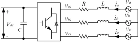
Fig. 1 shows schematics of the GCC, in which a dc-link capacitor appears on the left, and a three-phase voltage source, representing the voltage at the Point of Common Coupling (PCC) of the ac system, appears on the right. In this diagram the capacitor would be connected to the electrical generator (for example the wind turbine, or photovoltaic array) and has a dc voltage represented by Vdc, and the three voltages va, vb and vc would represent the

three-phase voltage of the electric power grid.

Figure 1: Grid-connected converter schematic.

The powers transferred between the grid and the converter include active power and reactive power. The purpose of the GCC controller is to control the active and reactive power transferred between the grid and the GCC.

The circuit contains 3-phase ac-voltagesva,vb, andvc, with corresponding

3-phase ac-currents ia, ib and ic. By transforming to a rotating frame of

vq. In this simpler d-q reference frame, the voltages and currents evolve

according to the following 2-dimensional vector differential equation (see Li et al. (2011, 2012) for further derivation):

vd vq =R id iq

+L∂ ∂t

id iq

+ωsL

−iq id

+

vd1

vq1

(1)

Here ωs is the angular frequency of the PCC voltage (i.e. the angular

fre-quency of the rotating dq reference frame, which is also the angular frefre-quency of the ac grid), and L and R are the inductance and resistance of the grid filter. vd1 andvq1 are the “control voltages” which are added into the system,

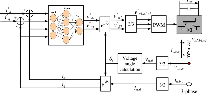
in the dq reference frame, through the GCC controller. The purpose of these control voltages is to influence the current transferred between the grid and the GCC, a process referred to asvector control. Fig. 2 shows schematics for the GCC controller, with a neural network to make the control decisions, plus circuits to transform both to and from the dq reference frame, as necessary, and a pulse-width-modulation (PWM) scheme to convert the neural-network control decisions to the high voltage control signals in the system. In the figure,θeis the instantaneous rotating angle of the three-phase grid voltage in the space vector domain.

PWM 3/2 3-phase supply 2/3 -

+ _v*

a1,b1,c1

v, v*1

v*1 v*d1

i*d

Vdc va,b,c e j

e

v*q1

3/2 i,

ia,b,c e j

e

From now on we will just consider the voltage and current variables in the simpler dq reference frame. The job of the GCC neural-controller is to output control voltages vd1 and vq1 which will make the actual dq-axis currents, id

and iq match as closely as possible some externally set reference currents, i∗d

and i∗_q.

Since the state variables areid and iq, Eq. (1) can be rearranged to give:

∂ ∂t id iq =−

R/L −ωs ωs R/L

id iq − 1 L

vd1−vd vq1−vq

(2)

For digital control implementations, a discrete-time equation is required:

id(kTs+Ts) iq(kTs+Ts)

=A

id(kTs) iq(kTs)

+B

vd1(kTs)−vd vq1(kTs)−vq

(3)

wherek is an integer time step,A is the system matrix, andB is the matrix associated with the control voltage. Our experiments used a zero-order-hold mechanism (Franklin et al., 1998) with sampling time Ts = 0.001 to obtain

the discrete-time equation (Eq. (3)) from the continuous-time one (Eq. (2)). This means the components of the matrices A and B are only available numerically.

Using conventional control-system notation, we define the state vector to be~x:=id

iq

, and the control vector to be~u:=vd1

vq1

(the “control voltages”), and~cto be a system vector (the “grid voltage”) defined by~c:=vd

vq

. Then, the system state evolution Eq. (3) can be written in a more concise form:

~xk+1 =A~xk+B(~uk−~c). (4)

2.1. A Basic NN Controller and Optimization Function

The tracking objective is to make the actual current state, ~xk, track the

given (possibly moving) target state ~x∗_k :=i∗_d

i∗

q

. Actions are chosen by

~

uk =kpwmπ(~xk, ~x∗k−~xk, ~w), (5)

between all pairs of layers. All nodes had a bias weight, and a hyperbolic tan-gent activation function. The input vectors were rescaled to be tanh(~xk/1000)

and tanh((~x∗_k−~xk)/100), respectively. We define the functionπ(·) to include

these input rescalings.

kpwm =Vdc/2 is a scalar constant, referred to as the gain of the voltage

source dc/ac PWM converter (Mohan et al., 2002). From a neural-network point of view, kpwm can be understood simply to be a constant for rescaling

the neural-network output. This will ensure each component of the action vector, ui, lies in the following range:

ui ∈[−kpwm, kpwm]. (6)

We train the weights of the action network to solve the tracking problem by doing gradient descent with respect to w~ on the following cost function:

J(~x0, ~w) := K−1

X

k=0

γkU(~xk, ~x∗k, ~uk) (7)

where

U(~xk, ~x∗k, ~uk) :=|~xk−~x∗k| m

(8)

andmis some constant power (we usedm= 1 in our experiments),|·|denotes the modulus of a vector, andγ ∈[0,1] is the constant discount factor (we used

γ = 1 throughout). The trajectory duration used for training was K = 1000 time steps (i.e. 1 second of real time). Lines 1-7 of Alg. 1 illustrate how Eqs. (4)-(8) can be used to simulate a single trajectory and calculate its total cost,

J.

To train the action network, we used BPTT, as described in the following subsection.

2.2. Backpropagation Through Time Algorithm

The action network was trained to minimize the cost in Eq. (7) by using BPTT (Werbos, 1990). BPTT efficiently calculates the gradient of J(~x0, ~w)

with respect to the weight vector of the action network, w~, for a given tra-jectory with arbitrary initial state ~x0. This gradient can thus be used to

Algorithm 1 BPTT for tracking control problem, with fixed A and B ma-trices

1: J ←0

2: {Unroll a full trajectory:}

3: for k = 0 to K−1 do

4: ~uk←kpwmπ(~xk, ~x∗k−~xk, ~w) {Neural-network output}

5: ~xk+1 ←A~xk+B(~uk−~c) {Calculate next state}

6: J ←J+γkU(x~k, ~x∗k, ~uk)

7: end for

8: {Backwards pass along trajectory:}

9: J ~w←~0

10: J ~xK ←~0

11: for k =K−1 to 0 step −1do

12: J ~uk ←(BT)J ~xk+1+γk

_∂U(~x

k,~x∗k,~uk)

∂~uk

13: J ~xk ←kpwm

_dπ(~x

k,~x∗k−~xk, ~w)

d~xk

J ~uk+ (AT)J ~xk+1+γk

_∂U(~x

k,~x∗k,~uk)

∂~xk

14: J ~w←J ~w+kpwm

_∂π(~x

k,~x∗k−~xk, ~w)

∂ ~w

J ~uk

15: end for

which accumulates the gradient-descent derivative. Alg. 1 gives pseudocode for both stages of this process.

The second half of the algorithm calculates the desired gradient, _{∂ ~}∂J_w. In this code, the variables J ~xk,J ~uk and J ~w are workspace column vectors of

dimension 2, 2, and dim(w~), respectively. These variables hold the “ordered partial derivatives” of J with respect to the given variable name, so that for example J ~xk = ∂

+_J

∂~xk. This ordered partial derivative, as defined by Werbos (Werbos, 1990; Werbos et al., 1992), represents the derivative of J with respect to~xk, assuming all other variables which depend upon~xk in lines 3-7

of Alg. 1 are not fixed, and thus their derivatives will influence the value of

∂+J

∂~xk via the chain rule. The derivation of the gradient computation part of the algorithm (lines 8-16) is exact, using the method known as generalized backpropagation (Werbos, 1990), or automatic-differentiation (Werbos, 2005; Rall, 1981). For full details of this derivation, see Werbos et al. (1992).

The vector and matrix notation is such that all vectors are columns and differentiation of a scalar by a vector gives a column. Differentiation of a vector function by a vector argument gives a matrix defined by the transpose of the usual Jacobian notation, such that for example, _{∂ ~}∂π_wij := ∂π_{∂ ~w}ji.

The algorithm refers to the derivatives ∂π_∂~x and _{∂ ~}∂π_w. These would be cal-culated by ordinary neural-network backpropagation. These derivatives are only required as an inner product with the vector J ~uk, and thus each

evalu-ation of these derivatives could be performed in asymptotic time O dim(w~). These neural-network backpropagation calculations should be considered as a sub-module necessary to implement Alg.1, and should not be confused with the BPTT backpropagation itself, which is what the rest of Alg. 1 imple-ments. Therefore the asymptotic running time for the whole BPTT algorithm applied to a full trajectory with K time steps will be O Kdim(w~).

The algorithm also refers to the derivatives ∂U_∂~x and ∂U_∂~u. By differentiating Eq. (8) directly, these are given by

∂U ∂~xk

=m(~xk−~x∗k)U 1−2/m

and,

∂U ∂~uk

2.3. Training the Neural Controller

We first trained the network to control the plant in a situation where the

A and B matrices were fixed. To choose these constants, we employed a standard arrangement for the integrated GCC and grid system, as used in renewable energy conversion system applications (Mullane et al., 2005; Pena et al., 1996; Li et al., 2011). These include 1) a three-phase 60Hz, 690V voltage source signifying the grid (i.e. ωs = 120π,

vd

vq

= 690V 0V

), 2) a reference voltage of 1200V for Vdc, and 3) a normal resistance ofR = 0.012Ω

and a normal inductance L= 0.002H for the grid filter. These constants are used to calculate the fixed A and B matrices in Eq. (3).

For training purposes, the reference current~x∗ :=i∗d

i∗

q

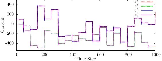
was changed every 0.05s (i.e. every 50 time steps), within the range [−500A,500A], in a fixed pattern. Fig. 3 shows this reference-current trajectory used for training. The objective of training is to make the actual trajectory match this reference trajectory, by minimization of Eq. (7). The actual trajectory was made to start from a fixed point, chosen arbitrarily to be ~x= [120

10 ].

-400 -200 0 200 400

0 200 400 600 800 1000

Curren

t

Time Step

i∗

d i∗

q id iq

Figure 3: Training data and neural-network output in the GCC tracking problem. The dotted lines indicate the reference currents that were used during training, and how these varied over the one-second training trajectory. The solid lines show the performance of the trained neural network (trained using a stabilization matrix, as described in Sec. 3.2) in controlling the actual currents, which lie very closely on top of the reference current curve, indicating that the tracking performance is good.

sta-bilization matrix). This was repeated for 10 different experiments. Each experiment started with a different initial neural-weights randomization in the range [−0.1,0.1].

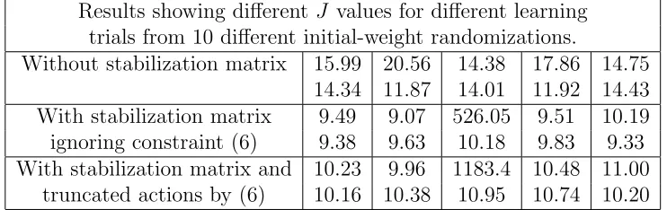
Table 1: Results with and without the “stabilization matrix”, with fixed knownAandB

matrices.

Results showing different J values for different learning trials from 10 different initial-weight randomizations.

Without stabilization matrix 15.99 20.56 14.38 17.86 14.75 14.34 11.87 14.01 11.92 14.43 With stabilization matrix 9.49 9.07 526.05 9.51 10.19 ignoring constraint (6) 9.38 9.63 10.18 9.83 9.33 With stabilization matrix and 10.23 9.96 1183.4 10.48 11.00

truncated actions by (6) 10.16 10.38 10.95 10.74 10.20

The neural controllers obtained by the best results in the first row of Table 1 replicate the neural controller performance described by Li et al. (2012), which can outperform PI and ACD methods in tracking ability (as we will show in the experiments of Section 5.1). As can be seen in the table, the results are not as good as when the stabilization-matrix method, described in the next section, is used.

3. Training Neural Network with a Stabilization Matrix

As indicated in Section 1, the control of a GCC normally faces the chal-lenges of rapidly changing target states, random variation of system param-eters, and oscillation of grid voltage. These issues cause a difficulties in training the action network to meet a variety of GCC control requirements. In this section we consider RNN action networks, and look at making more robust RNN controllers by trying to solve the problem of “exploding gradi-ents”, through the introduction of the stabilization matrix.

3.1. Why is training the action network so hard?

~ xk+1

k←k+ 1

~ xk ~ uk ~

xk

Action

Net

w

ork:

equation

(5)

Plan

t

Mo

del:

equation

(4)

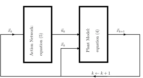
Figure 4: Power plant recurrence

is that each changed action (∆~uk) will consequently change the next state

(∆~xk+1) the system passes through, by Eq. (4). And each changed state

will further change the next action chosen, ∆~uk+1, by Eq. (5). Clearly this

creates an on-going cascade of changes. Hence changing one component of

~

w, even by the tiniest finite amount, can completely scramble the trajectory generated by Eqs. (4)-(5). This feedback is shown in Fig. 4. This difficulty is analogous to one of the major difficulties in training RNNs, since the model Eq. (4) can be interpreted to be just another layer of a neural network. In that case Fig. 4 becomes identical to the schematics of a RNN.

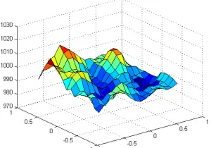
Consequently the function J(~x, ~w) can be over-sensitive to tiny changes inw~, chaotic even. In other words, the surface of the function inw~-space can be extremely crinkly, as illustrated by Fig. 5(a). Gradient-descent methods find it hard to traverse such a rugged surface, and hence it is difficult to train the action network effectively. This is one major reason why training the action network, or any recurrent network, is hard. This is referred to as the problem of “exploding” gradients by Hochreiter and Schmidhuber (1997). Our approach of using a stabilization matrix attempts to smooth out the surface of Fig. 5(a).

3.2. Using the stabilization matrix

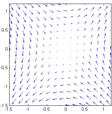
Fig. 6 shows the way the state vector would evolve if the action ~u ≡~0 and if ~c ≡ ~_{0, i.e. if the action network chose completely passive actions.}

In this case the state vector would drift around the state space like a cork floating on an ocean current.

(a) An error surface that is difficult for gradient-descent algorithms.

(b) A smooth error surface that is easy for gradient-descent algo-rithms.

Figure 5: Types of error surfaces commonly encountered. In our problem this is the surface of the function J(~x, ~w) inw~ space.

which will most likely take the state away from the target state ~x∗. Then, secondly, to actively head towards the tracking target point ~x∗. The idea of the stabilization matrix is to make the first of these two objectives automatic. This should make the action network’s task much simpler. The presence of the stability matrix should make the arrows in Fig. 6 vanish.

To achieve this, we first find the fixed point of Eq. (4) with respect to the control action by:

~

x=A~x+B(~u−~c)

~_{0 = (A−I)~x+B(~u−~c)}

~

u−~c=−B−1(A−I)~x

~

u=−B−1(A−I)~x+~c

where Iis the identity matrix.

Choosing this action will keep the plant in exactly the same state. Hence we change the action chosen by the action network from Eq. (5) into Eq. (9):

~

Figure 6: The motion which would occur from the equation∂~_∂kx =A~x+B(u~−~c) if~u−~c≡~_0.

In this case the motion simplifies to ∂~_∂kx =A~x.

where

W0 =−B−1(A−I) (10)

is the constant “stabilization matrix”, andπ(~x, ~x∗−~x, ~w) is the output of the neural network. W0 acts like an extra weight matrix in the neural network

that connects the input layer directly to the output layer. By the phrase “the stabilization matrix”, we mean both the W0 and ~c terms in Eq. (9). This

combination can be justified since ~ccould be included into the stabilization matrix as a bias term, as is conventional in neural networks.

The stabilization matrix effectively is a hand-picked weight matrix which helps the neural network do its job more easily. It aims to give the controller a default behavior of being able to hold the system-state steady. This should minimize the on-going cascade of changes that was described in the previ-ous subsection as making training the action network difficult. Hence the stabilization matrix aims to smooth out the crinkles of the J(~x, ~w) surface; making the surface more like Fig.5(b) than Fig. 5(a).

Results for the stabilization-matrix method are shown in Table 1. The results corresponding to the middle row of this table are displayed graphically as the solid curves in Fig. 3.

costs using this constraint are given in the third row of the table. In this case, the same fully-trained neural networks created for row 2 of the table were used again, but in reporting the final trajectory costs, the trajectories were generated while enforcing Eq. (6) through direct truncation of each component of ~uk.

Comparing the results using the stabilization matrix in the third row of the table, to the results without the stabilization matrix (given in the first row of the same table) we can see that using the stabilization matrix has produced consistently lower J values (ignoring the single extreme outlier). This is thought to be for the reasons given above. Further results also showing the effectiveness of the stabilization matrix are presented in Section 4.2.

The stabilization-matrix method has improved learning performance, and it was designed to do this by making the optimization surface smoother and therefore easier to navigate. Of course more sophisticated learning optimizers might be able to navigate a crinkly surface better than RPROP did (such as the multi-stream extended Kalman filter algorithm (Feldkamp and Puskorius, 1998), or conjugate gradient descent), but it would be expected that the stabilization-matrix method would assist these second-order algorithms to achieve better RNNs than they otherwise would.

4. Producing Adaptive Behaviour: Learning off-line to be adaptive on-line

The previous results are valid for a fixed inductance constant,L, and fixed grid voltage~c. However, when Lor~c vary, theA and Bmatrices in Eq. (4) will also change, and so the fixed behavior learned by the action network will no longer be optimal, and not solve the tracking problem correctly. Fig. 7 shows the resulting constant tracking error in several cases when L differs from the L = 2mH value used in training. In this section we describe how to remedy this, by creating a neural network that can adapt to changing unknown A and B matrices.

4.1. Adaptive control with variable L

(a) d-axis current (b) q-axis current

Figure 7: Constant tracking-error problem. The curves are all meant to lie on top of the “reference” curve (the tracking target). However only the L= 2mH curve does this properly; theL= 2.6mH andL= 1.4mH curves show a constant tracking error, especially noticeable in theq-axis. This problem is caused by the action network’s inability to adapt to the unknown and changing value of the constant L.

retraining, unlike traditional ACD methods which require continuous on-line training. Hence we are training the controller off-line to be adaptive on-line, following Prokhorov et al. (2002).

In this experiment, to train an adaptive controller, we regularly cycle the L values through a sequence, such as L = 2mH, L = 2.6mH, and L = 1.4mH, changing every 0.1 seconds, so the controller can learn to adapt to a standard range of conditions. Since the L value depends on the time step

k, we can denote the time dependent L value as Lk, and the corresponding

time dependent A and B matrix values asAk and Bk.

The adaptive behavior tracking problem would easily be solved if we were allowed to define the action network as π(~xk, ~x∗k, Lk, ~w), but the value

of Lk is hard to observe in reality and thus the neural network must deduce

it for itself. In addition, we must not change the W0 stabilization matrix

depending on Lk; since Lk is unknown to the neural controller, W0 must

remain constant.

Summarizing, when we switch to variable Lk, the problem of

by a constant tracking error in Fig. 7.

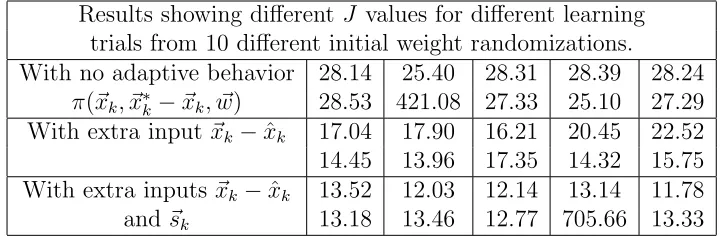
Table 2: Results for adaptive behavior controllers. All are using the fixed stabilization matrix, ignoring constraint (6), with changing unknownAk andBk matrices.

Results showing different J values for different learning trials from 10 different initial weight randomizations.

With no adaptive behavior 28.14 25.40 28.31 28.39 28.24

π(~xk, ~x∗k−~xk, ~w) 28.53 421.08 27.33 25.10 27.29

With extra input~xk−xˆk 17.04 17.90 16.21 20.45 22.52

14.45 13.96 17.35 14.32 15.75 With extra inputs~xk−xˆk 13.52 12.03 12.14 13.14 11.78

and~sk 13.18 13.46 12.77 705.66 13.33

To make the neural network become adaptive, it needs to have some idea on how the actual plant behavior is differing from its expected behavior, so that the controller can recalibrate its behavior intelligently during run time, and try to eliminate the constant tracking error shown in Fig. 7. For example, if we consider the situation of the controller representing a marksman shooting at a target under strong cross-wind conditions, then by observing the deflection the wind causes to the first shot, the marksman can make a compensatory adjustment to the subsequent shooting angle to try to cancel out the effect of the wind. Hence we give the neural network an extra input ~xk−xˆk which reflects the difference between the actual current state

(~xk) and the predicted current state (ˆxk) calculated with the fixed model,

such that ˆxk is defined by:

ˆ

xk := ¯A~xk−1+ ¯B(~uk−1−~c), (11)

where ¯Aand ¯Bare constant matrices of (4) chosen for the default L= 2mH value. In the real plant, Lk often differs from this default value, and so the Ak and Bk matrices will differ from ¯A and ¯B. Hence the difference~xk−xˆk

will be non-zero, and it will give useful feedback for telling the controller how to adapt to the dynamically changing plant conditions.

Adding this extra input~xk−xˆk to the neural network changes the

argu-ments of its function π(~xk, ~x∗k−~xk, ~w) into π(~xk, ~x∗k−~xk, ~xk−xˆk, ~w). This

2, which show a big improvement over the previous row. In this case, and in the following experiments, the stabilization matrix is defined by the fixed

¯

A and ¯B matrices, i.e. W0 :=−B¯−1( ¯A−I), since the changing Ak and Bk

matrices are not known to the controller. Also, the new input was rescaled into tanh ~xk−ˆxk

1000

and this extra vector input meant the neural-network ar-chitecture needed modifying to now have 6 input units.

Theorem 1 in Appendix A proves that adding this as an extra input is sufficient, in principle, to fix the constant tracking-error problem previously seen, under any mild unknown perturbations to the system and control ma-trices A and B, and under various tight assumptions stated in the theorem. In practice good action-network performance holds under more liberal con-ditions than those listed in the theorem, as the results in this section and the experiments of Section 5 show. Furthermore, Theorem 2 in the appendix shows that it is not possible to solve the problem if this extra input is re-moved.

Finally, to enhance performance further, an extra neural input pair is used to describe the previous action taken, ~uk−1. This allows the network

to observe whether this previous action led to the anticipated outcome in

~

xk −xˆk, and if not, an appropriate adjustment could be made to the next

action, ~uk, to compensate for this unexpected behavior. This is explicitly

to handle the uncertainty in the Bk matrix. To ensure this new input was

rescaled suitably, and also to avoid the scrambling effect of the stabilization matrix, we used the previous direct output of the neural-network function

π(·), instead of the output of Eq. (9). Lines 4, 5 and 8 of Alg. 2 give the exact details of how this new input was calculated.

We stress that this input, which we denote ~sk, was not intended to act

as a general purpose “context” unit such as is conventionally used in RNN architectures. Unlike a conventional context unit, our input~skis heavily

show. If a more complicated plant was to be controlled then more elaborate feedback units could be introduced, as and when required.

Combining all of these new features, i.e. the two extra neural input pairs to allow adaptive behavior, plus the stabilization matrix, means a trajectory can now be generated by lines 1-10 of Alg. 2. Adding these features changes the results to those shown in the final row of Table 2, which shows a further improvement over the previous row (ignoring the single extreme outlier re-sult). Of course, the performance under changing L is always going to be a bit worse than with fixed L (Table 1), since it is always going to take some time for the neural network to make enough observations of the plant’s actual behavior to deduce the values of the changing hidden matrices Ak and Bk.

However, we show in Section 5.2 that the neural controller is able to make an almost instantaneous adaptation to the plant’s changing conditions, and a virtual elimination of the constant tracking error previously shown.

The pseudocode in Alg. 2 gives the correct gradient calculation by BPTT, which was again generated using the method of Werbos et al. (1992). With both of the new extra neural input pairs, the final MLP has dimensions 8-6-6-2.

4.2. Effectiveness of the stabilization matrix in the adaptive control

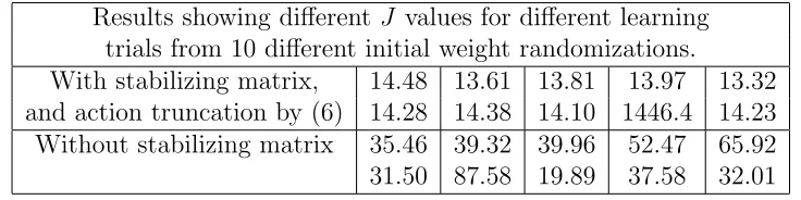
All of the experiments in the previous subsection used the stabilization-matrix method to enhance neural training– without it the results deteriorate significantly, as can be seen in Table 3. This is further evidence that the crinkly error surface is being smoothed out by the stabilization matrix.

Table 3: Effect of the stabilizing matrix on the adaptive behavior controllers. All are using the extra inputs ~xk−xˆk and~sk, for the vector-control problem with changing unknown Ak andBk matrices.

Results showing different J values for different learning trials from 10 different initial weight randomizations.

With stabilizing matrix, 14.48 13.61 13.81 13.97 13.32 and action truncation by (6) 14.28 14.38 14.10 1446.4 14.23 Without stabilizing matrix 35.46 39.32 39.96 52.47 65.92 31.50 87.58 19.89 37.58 32.01

Of course the stabilization matrixW0was only calculated for the constant

Algorithm 2Enhanced BPTT for tracking control problem, with time vary-ing A and B matrices, using a stabilization matrix and adaptive controller

1: J ←0, ˆx0 ←x~0,~s0 ←~0

2: {Unroll a full trajectory:}

3: for k = 0 to K−1 do

4: ~yk ←π(x~k, ~x∗k−~xk, ~xk−xˆk, ~sk, ~w) {Neural-network output}

5: ~uk←kpwm~yk+W0~xk+~c {Stabilized control action}

6: ~xk+1 ←Ak~xk+Bk(~uk−~c){Next state, using the time dependent Ak

and Bk matrices}

7: xˆk+1 ←A~¯xk+B¯(~uk−~c){Predicted next state, according to the fixed ¯

A and B¯ matrices}

8: ~sk+1 ←y~k {Previous network output}

9: J ←J+γkU(x~k, ~x∗k, ~uk)

10: end for

11: {Backwards pass along trajectory:}

12: J ~w←~0

13: J ~xK ←~0, J xˆK ←~0, J ~sK ←~0

14: for k =K−1 to 0 step −1do

15: J ~uk ←(Bk)TJ ~xk+1+B¯TJ xˆk+1+γk

_∂U(~x

k,~x∗k,~uk)

∂~uk

16: J ~y_k←kpwmJ ~uk+J ~sk+1

17: J ~xk ←

_dπ(~x

k,~x∗k−~xk,~xk−ˆxk,~sk, ~w)

d~xk

J ~y_k + W0TJ ~uk + (Ak)TJ ~xk+1 +

¯ AT_{J xˆ}

k+1+γk

_∂U(~x

k,~x∗k,~uk)

∂~xk

18: J xˆk ←

_∂π(~x

k,~x∗k−~xk,~xk−xˆk,~sk, ~w)

∂ˆxk

J ~y_k

19: J ~sk←

_∂π(~x

k,~x∗k−~xk,~xk−ˆxk,~sk, ~w)

∂~sk

J ~y_k

20: J ~w←J ~w+∂π(~xk,~x∗k−~xk,~xk−xˆk,~sk, ~w)

∂ ~w

J ~y_k

21: end for

different value. But it seems that the stabilization matrix was still effective in improving results on this problem. It remains to be seen how different the matrices Aand Bcan become before the stabilization matrix stops working. Fig. 8. shows the average cost per trajectory time step for successful trainings of the action network corresponding to the four conditions shown in Table 2 and 3, i.e., without stabilization matrix (case 1), with stabilization matrix (case 2), with extra input ~xk −xˆk (case 3), and with extra inputs ~

xk −xˆk and ~sk (case 4). As the figure indicates, without the stabilization

matrix, it is hard for the neural network to learn; but the overall average cost dropped to a small number very quickly with the stabilization matrix and the extra inputs~xk−xˆk and~sk.

Figure 8: Average cost per trajectory time step for training neural controller

5. Simulation Experiments

is included which demonstrates how the stabilization matrix can also be used when the B matrix is non-invertible.

5.1. Comparison of Neural Controller with Conventional Standard and DCC Vector-Control Mechanisms

In this comparison study, the performance of the neural controller is com-pared against standard PI controllers, under the same plant conditions as described in Section 2.3 (i.e. no adaptation to changing plant behavior was required). Fig. 9 shows the results. One of the result curves is for the neu-ral controller, another is for a tuned PI conventional GCC controller (Luo et al., 2009; Carrasco et al., 2006; Dannehl et al., 2009), and a third is for a “direct-current vector control” structure (DCC, (Li et al., 2010, 2011)). The PI controllers were tuned until the controller performance was acceptable (Li et al., 2011). The reference currents are given a step-change at 0.5s into the experiment, as shown in the figure.

(a) d-axis current (b) q-axis current

Figure 9: Comparison of two PI controllers (“conventional”, and “DCC”) with the neural vector controller.

5.2. Control Evaluation under Variable Parameters of GCC System

The previous experiment was for fixed A and B matrices. We now see how the controller can adapt when these matrices drift from their original values. Fig. 10 compares how the neural controller is affected when there is an increase or a decrease of inductanceLby 30% from its nominal value. For all the cases, a disturbance voltage ∆vd

∆vq

is also added to the grid voltage, and Eq. (9) is used to compute the final control voltage applied to the system. The results of Fig. 10 show a virtual elimination of the constant tracking error previously seen in Fig. 7, and the neural controller successfully making almost-instantaneous adaptation (with almost zero rise time and settling time) to the changing L, Ak and Bk system variables, with an adequate

overshoot. The results show successful tracking over a larger (and therefore more challenging) range of reference current values (i∗_d ∈ [−400,100], i∗_q ∈ [−100,0]) than was attempted in Fig. 7.

This experiment shows the RNN is successfully making adaptation to the changing plant behavior, while maintaining the tight tracking of the reference current that was seen in the previous experiment.

(a) L= 2.6mH, ∆vd =−0.3∗vd,

∆vq =−0.1∗vd

(b)L = 1.4mH, ∆vd =−0.3∗vd,

∆vq =−0.1∗vd

Figure 10: Performance of neural vector controller under variable grid-filter inductance and PCC voltage conditions.

5.3. Ability to Track Fluctuating Reference Current

such conditions, a variable d-axis reference current is generated while the q-axis reference current is set at zero (i.e., zero reactive power), with the standard fixed inductance value, L = 2mH. Fig. 11 shows that the neural network, with the stabilization matrix, predictive error signal ~xk−xˆk, and

control action history~sk, performs a near perfect match to the rapidly

chang-ing reference current. This kind of rapid close trackchang-ing would not be possible by PI controllers, as indicated by their sluggish performance in the previous experiments (e.g. Fig. 9).

Figure 11: Performance of neural vector controller under a variable reference current condition.

5.4. Experiment with Non-invertible Control Matrix

We now present an experiment where the matrix B is rectangular and non-invertible. The system considered here is taken from (Kirk, 2004, Ex.5.2-3):

∂~x ∂t =

0 1

2 −1

~ x+

0 1

u, (12)

for a state vector~x:=_x0

x1

and controlu∈ <. This equation was discretized using a sampling time Ts = 0.01, producing matrices A and B analogous

to those used in Eq. (3). Since B is square here, and therefore non-invertible, in order to use the stabilization matrix, we replaced the matrix inverse operation in Eq. (10) by the Moore-Penrose pseudoinverse (Golub and Van Loan, 1983) to obtain the results in the following experiment.

The problem is to optimize the cost-to-go functionJ (Eq. 7) for,

U(~xk, ~x∗k, ~uk) := x0(k)−1

2

Optimizing this cost function will move the state vector towards x0 _{= 1 as}

quickly as possible, while also penalizing excessively large actions u. Al-though this cost function does not explicitly specify a target for the state vector component x1_{, an implicit target for it is x}1 _{= 0, since the only way}

to obtain a fixed point of Eq. (12) is by achieving x1 _{= 0. Hence in this}

problem, the reference state can be considered to be~x∗ = [1 0].

The action network had a layered structure 4-6-1, with bias-weights for each node, extra short-cut connections from the input to the output layer, hyperbolic tangent activation functions at all network nodes, and weights initially randomized in the range [−.1, .1]. The 4 inputs to the neural network were tanh(~xk/10) and tanh(~x∗k−~xk). The output of the neural networkywas

used to generate the action via the relationshipu= 10ywhen no stabilization matrix was used, andu= 10y+W0~xwhen the stabilization matrix was used.

The trajectory start state was always~x= [2

1], and the trajectory duration

was 3 seconds (i.e. 300 time steps), with discount factor γ = 1. In this problem no adaptive behaviour was required, since theAandBmatrices are fixed and known. Training took place for 800 iterations, from 10 different random weight initializations, using BPTT with RPROP, both with and without a stabilization matrix. The exact derivatives of Eq. (13) were made available to the BPTT algorithm. Results are shown in Table 4 and Fig. 12 shows a trajectory generated with the stabilization matrix, i.e. effectively solving the problem by following the reference state ~x∗.

Table 4: Results with and without the “stabilization matrix”, for the problem defined in Sec. 5.4.

Results showing different J values for different learning trials from 10 different initial weight randomizations.

Without stabilization matrix 0.2508 0.2508 0.2508 0.2506 0.2507 0.2507 0.2508 0.2507 0.2509 0.2508 With stabilization matrix 0.2030 0.2030 0.2030 0.2029 0.2029 0.2039 0.2029 0.2028 0.2029 0.2029

6. Conclusions

-2 -1 0 1 2 3

0 50 100 150 200 250 300

~x

Time Step

x∗0

x∗1

x0

x1

Figure 12: Trajectory after training with a stabilization matrix, for the problem defined in Sec. 5.4.

electric power system applications. We described how conventional neural controllers, which require on-line retraining to achieve their adaptation, can have limitations in adaptation speed and convergence. In contrast, the con-troller we have proposed does not need any on-line retraining, and can adapt effectively and almost instantaneously to changing plant conditions and/or changing reference commands. Compared to standard vector-control meth-ods, including recently developed direct-current vector-control techniques, the neural vector-control approach produces good response time, low over-shoot, and in general, excellent performance.

We have proposed some novel RNN inputs that allow for rapid adap-tation and have discussed the motivations for using these unusual inputs as opposed to conventional generic context units. We have also introduced the stabilization-matrix method to ease RNN training in these experiments. The benefits of this method have been shown in numerical experiments, in Sections 3 to 5, in the case-study GCC problem and in a different problem domain demonstrating a situation with a non-invertible control matrix. It is our contention that this RNN controller architecture can have generic control applications to other kinds of plant, and produce a competitive alternative method to ACD and PI controllers.

“vanishing” gradients (Hochreiter and Schmidhuber, 1997), or superior opti-mizers (Feldkamp and Puskorius, 1998). We have described how the method we proposed can be used in conjunction with these more powerful optimizers. In this research we have concentrated on situations where the A and B

matrices are fixed or changing with small deviations over time. In future research, it will be necessary to investigate more problem domains including situations where the A and B matrices are functions of both~xand t.

Appendix A. Proof of sufficiency of the arguments chosen to solve the adaptive tracking problem

In this appendix, in Theorem 1 we prove that a neural network with inputs (~x∗_k−~xk) and (~xk−xˆk) is theoretically capable of solving the tracking

problem, under mildly perturbed system and control matrices, A and B. In Theorem 2 we show that it is not possible for a neural network with only the inputs ~xk and~x∗k to solve the same problem.

Theorem 1. A neural network of the form π(~xk, ~x∗k −x~k, ~xk −xˆk, ~w) can

solve the tracking problem for some unknown constant system matricesAand

B, which are suitably close approximations to some known constant system

matrices A¯ and B¯, if the following 4 conditions are all met:

1. The known constant matrices A¯ and B¯ are sufficiently close

approxi-mations to the unknown constant matrices A and B.

2. The matrix B¯ is square and invertible.

3. The tracking target ~x∗ is sufficiently slowly moving such that it can be

treated as constant.

4. The discrete-time matricesA¯ andB¯ were generated from an underlying

continuous-time process with sufficiently small sampling time.

Proof. The proof is split into two steps. Firstly, in “Proof Part-A”, it is proven that we can simplify the situation to the case where both A¯ and B¯

are equal to identity matrices. Secondly, in “Proof Part-B”, this simplified situation is analysed and a choice of action, constructed only from the argu-ments to the neural network, is proven to make the system state~xk converge

to the tracking target ~x∗.

thatA:=A¯+A∆andB:=B¯+B∆. Under this notation, the state-evolution

equation (4) changes into

~

xk+1 = (A¯ +A∆)~xk+ (B¯ +B∆)(~uk−~c). (A.1)

Also, by Condition 3, we can assume the tracking target ~x∗_k is fixed and hence drop the k subscript and just use~x∗.

The two main proof parts now follow:

Proof Part-A. We define a transformed control vector~vk, which is related

to the original control vector ~uk by the relationship:

~uk=B¯−1 ~vk−(A¯ −I)~xk

+~c. (A.2)

Substituting this into (A.1) gives:

~

xk+1 =(A¯ +A∆)~xk+ (B¯ +B∆)B¯−1 ~vk−(A¯ −I)~xk

(by (A.2))

=(A¯ +A∆)~xk+ (~vk−(A¯ −I)x~k) +B∆B¯−1 ~vk−(A¯ −I)~xk

=(A∆)~xk+ (~vk+~xk) +B∆B¯−1 ~vk−(A¯ −I)~xk

= I+A∆−B∆B¯−1(A¯ −I)

~

xk+ I+B∆B¯−1

~vk

= (I+A0_∆)~xk+ (I+B0∆)~vk (A.3)

where

A0_∆:=A∆−B∆B¯−1(A¯ −I), (A.4)

and

B0_∆:=B∆B¯−1. (A.5)

Therefore we only need consider control systems of the form (A.3). ~vk

is now the control vector. Next we must show that the two perturbation matrices, A0_∆ and B0_∆, in (A.3) are both small.

The matrices A¯ and B¯ were derived from an exact discrete-time system of the form of Eq. (4), i.e.

which itself was derived from an underlying continuous-time system, of the form of Eq. (2),

∂~x(t)

∂t =F~x(t) +G(~u(t)−~c), (A.7)

with sampling time Ts.

Note that the discrete-time system (Eq. (A.6)) is related to the continuous-time system (Eq. (A.7)) by a first-order Taylor-series expansion, as follows:

~xk+1 =~xk+ ∂~x

∂tTs+ O (Ts)

2

=~xk+ (F~xk+G(u~k−~c))Ts+ O (Ts)2

(by Eq. (A.7))

= (I+FTs)~xk+G(~uk−~c)Ts+ O (Ts)2

(A.8)

By comparing Eqs. (A.8) and (A.6), we can see that A¯ = I+FTs+

O (Ts)2

, and B¯ = GTs+ O (Ts)2

. Therefore as Ts → 0, we must have ¯

A→I and B¯ →0. Therefore by Condition 4, we have

¯

A−I≈0 (A.9)

Also, by Conditions 1 and 2, we have,1

B∆B¯−1 ≈0. (A.10)

We can now see thatA0_∆ is small, since all of the terms in equation (A.4) are small (by Eqs. (A.9) and (A.10) and Condition 1 which implies that both

A∆ and B∆ are small). Also, B0∆ is small too, by Eqs. (A.5) and (A.10).

So working with Eq. (A.3), we can relabelA0_∆ toA∆and B0∆ toB∆ and

~

v to~u, and therefore work with

~

xk+1 = (I+A∆)~xk+ (I+B∆)~uk, (A.11)

where both A∆ and B∆ are small. This equation is similar to (A.1), except

that we can now assume A¯ and B¯ are both identity matrices.

1_{This equation takes a bit of consideration, sinceT}

s→0 implies bothB∆ andB¯ have

magnitudes proportional toTs, and this will makeB¯−1large, implying a possible violation

of Eq. (A.10). However when the product B∆B¯−1 is formed, the two proportionalities

to Ts cancel each other, and therefore Ts does not influence the final magnitude of this

Proof Part-B. The simplified state-evolution equation is given by (A.11), or equivalently,

~

xk =(I+A∆)~xk−1+ (I+B∆)~uk−1. (A.12)

In this system (A.12), the “predicted” state defined by (11) simplifies down into:

ˆ

xk :=~xk−1+~uk−1. (A.13)

We now prove that it is possible to control the above system, assuming sufficiently small perturbation matrices A∆ and B∆, by making our action

choice a function of the inputs of the neural network, as follows. Consider the following choice of action, which is permitted because it is purely a function of the arguments of π(~xk, ~x∗k−~xk, ~xk−xˆk, ~w):

~

uk =(~x∗−~xk)−(~xk−xˆk) (A.14)

=~x∗−2~xk+x~k−1+~uk−1 (by (A.13))

=~x∗−2(~xk−1+A∆~xk−1+~uk−1+B∆~uk−1) +x~k−1+~uk−1 (by (A.12))

=~x∗−2~xk−1−2A∆~xk−1−2~uk−1−2B∆~uk−1+~xk−1 +~uk−1

=~x∗−~xk−1−2A∆~xk−1−~uk−1−2B∆~uk−1

=~x∗−(I+ 2A∆)~xk−1−(I+ 2B∆)~uk−1 (A.15)

Combining (A.12) and (A.15) into one discrete-time system gives:

~ xk ~ uk =E ~ xk−1

~ uk−1

+ 0 ~ x∗ (A.16) where E:=

(I+A∆) (I+B∆)

−(I+ 2A∆) −(I+ 2B∆)

. (A.17)

We must prove that (A.16) converges. Note that a fixed point of this is

~x∗ −(I+B∆)−1A∆~x∗

T

, because then

~ x∗

−(I+B∆)−1A∆~x∗

=E

~ x∗

−(I+B∆)−1A∆~x∗

This fixed point satisfies~xk=~x∗, so it is a correct solution to the tracking

problem.

So we next must show that this fixed point is an attractor. Substituting shifted coordinates~xk :=~x0k+~x

∗ _and~u

k :=~u0k−(I+B∆)−1A∆~x∗ into (A.16)

moves the fixed point to the origin:

~ x0_k+~x∗

~u0_k−(I+B∆)−1A∆~x∗

=E

~x0_k−1+~x∗

~u0_k−1−(I+B∆)−1A∆~x∗

+

0

~x∗

=E

~ x0_k−1 ~ u0_k−1

+E

~ x∗

−(I+B∆)−1A∆~x∗

+ 0 ~ x∗ =E ~ x0_k−1 ~ u0_k−1

+

~ x∗

−(I+B∆)−1A∆~x∗

(by Eq. (A.18))

⇒

~ x0_k ~ u0_k

=E

~ x0_k−1 ~ u0_k−1

(A.19)

Hence we just need to prove that (A.19) converges to the origin.

We split the matrix E in (A.17) into two parts: a core matrix C :=

I I

−I −I

and a small perturbation matrix P:= A∆ B∆ −2A∆−2B∆

, such that P+

C≡E, and also define ~yk :=

_~x0

k

~ u0_k

, so that (A.19) can be rewritten as

~

yk= (C+P)~yk−1.

Applying two steps of this iteration, and noting thatC2 ₌ I I

−I−I

_{I I}

−I−I

= (0 0

0 0), gives:

~

yk = (CP+PC+P2)~yk−2. (A.20)

Since every term in this product has a factor of P, which is assumed small, clearly this equation will converge to zero as k → ∞. This completes the proof that it is possible to solve the tracking problem using a function of the form π(~xk, ~x∗k−~xk, ~xk−xˆk, ~w), under the assumed conditions of the

theorem.

~

xk, ~xk−xˆk, ~w) is in any way optimal; just that this choice produces a possible

solution, which is guaranteed to converge to the tracking target, eventually, and under the given assumptions. In fact, the results in the third row of Table 2 show that additional inputs can improve tracking performance over the basic function considered in Theorem 1. These experiments also show the neural network can cope with fast-moving tracking targets (e.g. in Section 5.3), and finite Ts values, so the four strict conditions of this theorem may

be stretched, to a certain extent, in practical applications.

A key motivation of this proof has been to show that the disturbances to the A and B matrices can be to all matrix components, and tracking will still be possible provided those disturbances are sufficiently small.

Theorem 2. It is not possible for a feed-forward neural network with only

the inputs ~xk and ~x∗k to solve the tracking problem, when the system and

control matrices A and B have undergone a mild disturbance.

Proof. Suppose we had actions~uk generated by a function~uk :=π(~xk, ~x∗),

and suppose this control action was able to move the plant’s state vector to the tracking target ~x∗ and hold it there, so that ~xk = ~x∗ for all k > k0,

for some constant k0. At this target state, i.e. at ~xk+1 = ~xk = ~x∗, the

state-evolution equation, in the simplified frame of reference given by (A.11), becomes:

~

x∗ = (I+A∆)~x∗+ (I+B∆)~uk

⇒~uk =−(I+B∆)

−1

A∆~x∗

This is the action required to hold the plant at the target state, once there. So, when ~xk =~x∗, we must haveπ(~xk, ~x∗) equal to

π(~x∗, ~x∗) =−(I+B∆)

−1

A∆~x∗

The right-hand side (RHS) of this equation has a dependency on the pertur-bation matrices, A∆ and B∆. This means, in different plants with different

References

Barnard, E., 1993. Temporal-difference methods and markov models. IEEE Transactions on Systems, Man, and Cybernetics 23 (2), 357–365.

Bishop, C. M., 1995. Neural Networks for Pattern Recognition. Oxford Uni-versity Press.

Carrasco, J. M., Franquelo, L. G., Bialasiewicz, J. T., Galv´an, E., Guisado, R. C. P., Prats, M. A. M., Le´on, J., Moreno-Alfonso, N., August 2006. Power-electronic systems for the grid integration of renewable energy sources: A survey. IEEE Transactions on Industrial Electronics 53 (4), 1002–1016.

Dannehl, J., Wessels, C., Fuchs, F. W., October 2009. Limitations of voltage-oriented PI current control of grid-connected PWM rectifiers with lcl fil-ters. IEEE Transactions on Industrial Electronics 56 (2), 380–388.

Fairbank, M., Alonso, E., June 2012. The divergence of reinforcement learn-ing algorithms with value-iteration and function approximation. In: Pro-ceedings of the IEEE International Joint Conference on Neural Networks 2012 (IJCNN’12). IEEE Press, pp. 3070–3077.

Feldkamp, L. A., Puskorius, G. V., 1998. A signal processing framework based on dynamic neural networks with application to problems in adaptation, filtering, and classification. Proceedings of the IEEE 86 (11), 2259–2277.

Figueres, E., Garcer´a, G., Sandia, J., Gonzalez-Espin, F., Rubio, J. C., March 2009. Sensitivity study of the dynamics of three-phase photovoltaic invert-ers with an LCL grid filter. IEEE Transactions on Industrial Electronics 56 (3), 706–717.

Franklin, G. F., Workman, M. L., Powell, D., 1998. Digital control of dynamic systems, 3rd Edition. Addison-Wesley Longman Publishing Co., Inc.

Golub, G. H., Van Loan, C. F., 1983. Matrix Computations. Johns Hopkins University Press, Baltimore, Maryland.

Kirk, D. E., 2004. Optimal control theory: an introduction. Dover Publica-tions.

Li, S., Fairbank, M., Wunsch, D., Alonso, E., June 2012. Vector control of a grid-connected rectifier inverter using an artificial neural network. In: Proceedings of the IEEE International Joint Conference on Neural Networks 2012 (IJCNN’12). IEEE Press, pp. 1783–1789.

Li, S., Haskew, T. A., Hong, Y. K., Xu, L., February 2011. Direct-current vec-tor control of three-phase grid-connected rectifier-inverter. Electric Power Systems Research 81 (2), 357–366.

Li, S., Haskew, T. A., Xu, L., December 2010. Control of HVDC light sys-tem using conventional and direct current vector control approaches. IEEE Transactions on Power Electronics 25 (12), 3106–3118.

Luo, A., Tang, C., Shuai, Z., Tang, J., Xu, X. Y., Chen, D., July 2009. Fuzzy-PI-based direct-output-voltage control strategy for the STATCOM used in utility distribution systems. IEEE Transactions on Industrial Electronics 56 (7), 2401–2411.

Mohan, N., Undeland, T. M., Robbins, W. P., 2002. Power electronics: con-verters, applications, and design, 3rd Edition. John Wiley & Sons.

Mullane, A., Lightbody, G., Yacamini, R., November 2005. Wind-turbine fault ride-through enhancement. IEEE Transactions on Power Systems 20 (4), 1929–1937.

Park, J., Harley, R., Venayagamoorthy, G., 2004. New external neuro-controller for series capacitive reactance compensator in a power network. IEEE Transactions on Power Systems 19 (3), 1462–1472.

Pena, R., Clare, J. C., Asher, G. M., May 1996. Doubly fed induction generator using back-to-back PWM converters and its application to variable-speed wind-energy generation. In: Electric Power Applications, IEE Proceedings-. Vol. 143. IET, pp. 231–241.

Prokhorov, D. V., Feldkamp, L. A., Tyukin, I. Y., 2002. Adaptive behavior with fixed weights in RNNs: an overview. In: Proceedings of the 2002 In-ternational Joint Conference on Neural Networks, 2002. IJCNN’02. Vol. 3. IEEE, pp. 2018–2022.

Qiao, W., Harley, R., Venayagamoorthy, G., 2008a. Fault-tolerant optimal neurocontrol for a static synchronous series compensator connected to a power network. IEEE Transactions on Industry Applications 44 (1), 74–84.

Qiao, W., Harley, R. G., Venayagamoorthy, G. K., 2009a. Coordinated reac-tive power control of a large wind farm and a STATCOM using heuristic dynamic programming. IEEE Transactions on Energy Conversion 24 (2), 493–503.

Qiao, W., Venayagamoorthy, G. K., Harley, R. G., 2008b. Optimal wide-area monitoring and nonlinear adaptive coordinating neurocontrol of a power system with wind power integration and multiple FACTS devices. Neural Networks 21 (2), 466–475.

Qiao, W., Venayagamoorthy, G. K., Harley, R. G., 2009b. Real-time im-plementation of a STATCOM on a wind farm equipped with doubly fed induction generators. IEEE Transactions on Industry Applications 45 (1), 98–107.

Rabelo, B. C., Hofmann, W., da Silva, J. L., de Oliveira, R. G., Silva, S. R., October 2009. Reactive power control design in doubly fed induction gen-erators for wind turbines. IEEE Transactions on Industrial Electronics 56 (10), 4154–4162.

Rall, L. B., 1981. Automatic differentiation: Techniques and applications. Lecture Notes in Computer Science 120.

Riedmiller, M., Braun, H., 1993. A direct adaptive method for faster back-propagation learning: The RPROP algorithm. In: Proc. of the IEEE Intl. Conf. on Neural Networks. San Francisco, CA, pp. 586–591.

Venayagamoorthy, G. K., Harley, R. G., Wunsch, D. C., 2002. Comparison of heuristic dynamic programming and dual heuristic programming adaptive critics for neurocontrol of a turbogenerator. IEEE Transactions on Neural Networks 13 (3), 764–773.

Wang, C., Nehrir, M. H., November 2007. Short-time overloading capabil-ity and distributed generation applications of solid oxide fuel cells. IEEE Transactions on Energy Conversion 22 (4), 898–906.

Wang, F.-Y., Zhang, H., Liu, D., 2009. Adaptive dynamic programming: An introduction. IEEE Computational Intelligence Magazine 4 (2), 39–47.

Werbos, P. J., 1990. Backpropagation through time: What it does and how to do it. In: Proceedings of the IEEE. Vol. 78, No. 10. pp. 1550–1560.

Werbos, P. J., 1992. Approximating dynamic programming for real-time con-trol and neural modeling. In: White, Sofge (Eds.), Handbook of Intelligent Control. Van Nostrand Reinhold, New York, Ch. 13, pp. 493–525.

Werbos, P. J., 1998. Stable adaptive control using new critic designs. eprint arXiv:adap-org/9810001, sections 7.7–7.8.

Werbos, P. J., 2005. Backwards differentiation in AD and neural nets: Past links and new opportunities. In: B¨ucker, H. M., Corliss, G., Hovland, P., Naumann, U., Norris, B. (Eds.), Automatic Differentiation: Applications, Theory, and Implementations. Lecture Notes in Computational Science and Engineering. Springer, pp. 15–34.

Werbos, P. J., McAvoy, T., Su, T., 1992. Neural networks, system identi-fication, and control in the chemical process industries. In: White, Sofge (Eds.), Handbook of Intelligent Control. Van Nostrand Reinhold, New York, Ch. 10, sec. 10.6.1–10.6.2, pp. 339–343, version on author’s home-page with errata.

URL www.werbos.com