A novel algorithm for radar classification based on Doppler characteristics exploiting orthogonal pseudo-Zernike polynomials

A Novel Algorithm for Radar

Classification Based on

Doppler Characteristics

Exploiting Orthogonal

Pseudo-Zernike Polynomials

CARMINE CLEMENTE,Member, IEEE University of Strathclyde

Glasgow, UK

LUCA PALLOTTA,Student Member, IEEE ANTONIO DE MAIO,Fellow, IEEE Universit´a degli Studi di Napoli “Federico II” Naples, Italy

JOHN J. SORAGHAN,Senior Member, IEEE University of Strathclyde

Glasgow, UK

ALFONSO FARINA,Fellow, IEEE SELEX ES

Rome, Italy

Phase modulation induced by target micromotions introduces sidebands in the radar spectral signature returns. Time-frequency distributions facilitate the representation of such modulations in a micro-Doppler signature that is useful in the characterization and classification of targets. Reliable micro-Doppler signature classification requires the use of robust features that are capable of uniquely describing the micromotion. Moreover, future applications of micro-Doppler classification will require meaningful

representation of the observed target by using a limited set of values. In this paper, the application of the pseudo-Zernike moments for micro-Doppler classification is introduced. Specifically, the proposed algorithm consists of the extraction of the pseudo-Zernike moments from the cadence velocity diagram (CVD). The use of

pseudo-Zernike moments allows invariant features to be obtained

Manuscript received November 26, 2013; revised April 23, 2013, July 25, 2014; released for publication October 1, 2014.

DOI. No. 10.1109/TAES.2014.130762.

Refereeing of this contribution was handled by R. Adve.

This work is licensed under a Creative Commons Attribution 3.0 License. For more information, seehttp://creativecommons.org/licenses/by/3.0/.

Authors’ addresses: C. Clemente, University of Strathclyde, Dept. of Electronic and Electrical Engineering, 204 George Street, Glasgow, G1 1XW United Kingdom. E-mail: ([email protected]); L. Pallotta, A. De Maio, Universit´a degli Studi de Napoli, “Frederico II, via Claudio 21, Naples, Italy 80125. E-mail: ([email protected], [email protected]); A. Farina, SELEX ES,

via Tiburtina, Km.12.4, Rome I-00131, Italy. (E-mail: [email protected]).

0018-9251/15/$26.00C 2015 IEEE

that are able to discriminate the content of two-dimensional matrices with a small number of coefficients. The analysis has been conducted both on simulated and on real radar data, demonstrating the effectiveness of the proposed approach for classification purposes.

I. INTRODUCTION

Moving targets illuminated by a radar system introduce frequency modulations caused by the

time-varying delay that occurs between the target and the sensor. The main bulk translation of the target, towards or away from the sensor, induces a frequency shift of the echo as a result of the well-known Doppler effect. However, the target may contain parts that have additional movements with respect to the target main motion. These movements can contribute with frequency modulations around the main Doppler shift and they are commonly referred to as micro-Doppler modulations. It is important to underline that, in the open literature, an unambiguous definition of micro-Doppler effect is not present (see for instance [1–3,5]); consequently, within this paper we prefer to associate to the term micro-Doppler all the frequency modulations due to small displacement, rotation, or vibration of secondary parts of the object. The analysis of radar micro-Doppler was introduced by Chen in [4] and widely treated in [5], demonstrating the potential of micro-Doppler information for target classification and micromotion analysis. Over the last decade, the analysis of micro-Doppler signatures has been investigated for different families of radar systems [7], demonstrating the effectiveness of models and potential of such information source.

Micro-Doppler can be regarded as a unique signature of the target that provides additional information that is complementary to existing methods for target recognition. Specific applications include the recognition of space, air, and ground targets. Recently, novel technologies and techniques have opened a wider set of applications for micro-Doppler signatures, such as passive radar and acoustic micro-Doppler [8,9]. For example, micro-Doppler signatures can be used for human identification under different weather conditions. In particular, specific components of micro-Doppler gait signature can be related to parts of the body for

profile (MFP) based approach has been presented achieving good results with low complexity.

In this paper, we present a novel micro-Doppler signature extraction method that is based on the use of pseudo-Zernike moments [16]. The family of geometric moments represented by Hu [17], Zernike [18], and pseudo-Zernike [16], has been widely used in image processing for pattern recognition and image reconstruction [19–21]. These moments can provide potentially useful properties such as position, scale, and rotational invariance. Zernike moments, unlike Hu moments, are obtained using a set of orthogonal

polynomials, namely Zernike polynomials that comprise independent moments. This is an important property as independent moments allow us to obtain more information considering the same number of coefficients.

Pseudo-Zernike moments, introduced by Bhatia in [16], improve Zernike moments by reducing the noise sensitivity compared with Zernike moments and increasing the number of moments available for a given order of the polynomial. Consequently, the

pseudo-Zernike moments were selected as features to discriminate different micro-Doppler signatures, in the novel approach described in this paper.

The use of the pseudo-Zernike moments allows the introduction of important characteristics in the

representation of a micro-Doppler signature, in order to fit different requirements. In particular translational

invariance allows the unique identification of targets with different main Doppler shifts but belonging to the same class. The scale invariance allows us to provide features invariant with respect to variations of the aspect angle, making the algorithm applicable in a multistatic scenario without the requirement of a multistatic training dataset. The scale invariance can be also exploited to use a database acquired at a carrier frequency in an automatic target recognition (ATR) working with a slightly different one. Another advantage of the scale invariance for this specific problem is the capability of mitigating physical differences between targets of the same class (e.g. two people walking, a tall and a short one that would introduce different micro-Doppler shift that might lead to wrong classification). Moreover, in the proposed algorithm the pseudo-Zernike polynomials are computed starting from the CVD, thus introducing the advantage of robustness with respect to the initial phase of the micromotion and the opportunity to introduce the scene invariance by removing the zero periodicity component before computing the pseudo-Zernike moments.

The remainder of the paper is organized as follows. Section II introduces the pseudo-Zernike moments theory, and describes the novel feature extraction algorithm. The effectiveness of the proposed approach is demonstrated in Section III, where simulated data are used to justify the choice of the pseudo-Zernike moments, and in Section IV where accurate classification results on real Ku and X band data are presented. Section IV concludes the paper.

II. PSEUDO-ZERNIKE MOMENTS BASED FEATURES

In this section, a novel feature for radar micro-Doppler classification is introduced. The approach is based on the use of pseudo-Zernike moments [16], in order to obtain reliable feature vectors with relatively small dimension and low computational complexity. The novel feature benefits the specific properties of the pseudo-Zernike moments such as invariance with respect to translation and rotation. Moreover, the scale invariance can be included if required by the specific applications.

In the next subsections, the theory defining the pseudo-Zernike moments is introduced, followed by the novel feature extraction algorithm.

A. Pseudo-Zernike Moments

Letf(x, y) be a nonnegative real defined image, i.e.,

f(x, y)≥0. The moments off(x,y) of order (or degree)

n + lare defined as the projection of the functionf(x,y) on the monomialsxn_yl_{, by the integral [17]}

Mn,l =

R2

xnylf(x, y)dxdy. (1)

Notice that the low order moments share important properties that allow us to characterize an image. More specifically, the zero order moment defined as

M0,0 =

R2

f(x, y)dxdy, (2)

and the first order moments, given by

M1,0=

R2

xf(x, y)dxdy (3)

and

M0,1=

R2

yf(x, y)dxdy, (4)

are useful to represent the position of the image centroid [18], whose coordinates within the image can be computed as

Cx =M1,0/M0,0 and Cy =M0,1/M0,0. (5)

The moments described by(1)–(4)are not orthogonal because of the dependence on the family of monomials

{xn_yl_{}, which in general do not share orthogonality} properties.

Zernike polynomials are a set of orthogonal functions, with simple rotation properties [16,18], that can be written in the form

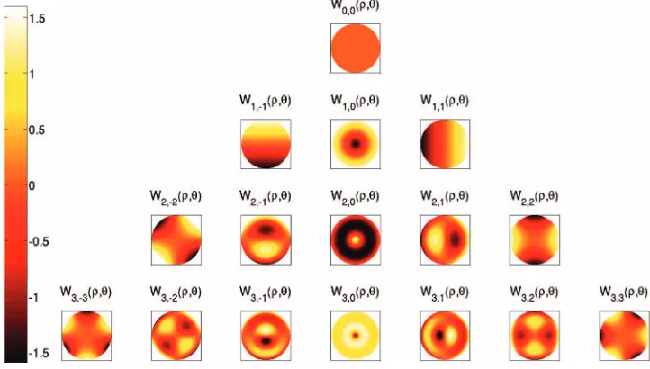
Vn,l(x, y)=Vn,l(ρcosθ, ρsinθ)=Rn,l(ρ)ej lθ, (6)

Fig. 1. Pseudo-Zernike polynomials for orders 0 to 3.

unit circle (i.e., forx2 + y2≤1), the orthogonality relation [16]

x2_+y2_≤1

V_n,l∗ (x, y)Vm,k(x, y)dxdy = π

n+1δmnδkl, (7)

where the symbol (·)∗indicates the complex conjugate operator, andδmnis the Kronecker delta function, i.e.,

δmn=

1 if m=n

0 if m=n.

As highlighted in [16], the radial polynomialsRn,l(ρ) exhibit the following explicit expressions

Rn,l(ρ)= (n−|l|)/2

k=0

(−1)k (n−k)!

k!

n+|l| 2 −k

!

n−|l|

2 −k

! ρn−2k,

(8) wheren≥0 andlare integers such thatn– |l| is even and

n≥|l|. Finally, the complex Zernike moments (obtained by projectingf(x,y) on the Zernike polynomials) are defined as

ζn,l =

n+1

π

x2_+y2_≤1

V_n,l∗ (ρ(x, y), θ(x, y))f(x, y)dxdy

=ζ_n,−l∗ . (9)

In a similar manner, in place of polynomials inxandy, as given in(6), it is also possible to consider polynomials in

x,y, andρ =x2_+y2_{[16]. In such a case, the} polynomials of orderncan be written in the following form

Wn,l(x, y, ρ)=Wn,l(ρcosθ, ρsinθ, ρ)=Sn,l(ρ)ej lθ, (10) wheren≥0 andlare integers such thatn≥|l|. For a more clear understanding,Fig. 1shows the pseudo-Zernike polynomialsWn,l(θ,ρ) with order fromn=0 ton=3.

Exploiting expression(10), the pseudo-Zernike moments are defined as

ψn,l =

n+1

π 2π

0 1

0

W_n,l∗ (ρ, θ)f(ρcosθ, ρsinθ)ρdρdθ,

(11) where the radial polynomials [16] are now expressed as

Sn,l(ρ)= n−|l|

k=0

(−1)k (2n+1−k)!

k! (n+|l|+1−k)! (n−|l|−k)!ρ n−k_.

(12) Notice that the number of linearly independent

pseudo-Zernike polynomials of degree≤nis (n + 1)2_, whereas for the Zernike polynomials, it is only

1

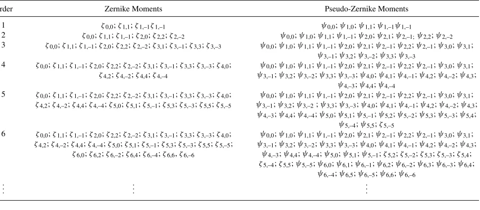
2(n+1)(n+2).Hence, having fixed the degree of the polynomial, the number of pseudo-Zernike moments (or coefficients) is much greater than that of Zernike. This is an important property of the pseudo-Zernike moments, as at parity of order much more information is provided using the pseudo-Zernike moments. Indeed, to obtain the same degree of information, a higher order of Zernike moments, with respect to pseudo-Zernike, is required, which reflects in a higher noise sensitivity. For each fixed orderTable Ishows the corresponding Zernike and pseudo-Zernike moments. Clearly the moments of a certain order contain all the moments of the lowest orders.

An important characteristic of Zernike and pseudo-Zernike moments is the simple rotational transformation property, as a result of the fact that computing the moments only requires a phase factor on the rotation of axes [16,18]. The latter is due to the fact that the polynomials can be written in the forms(6)and

TABLE I

Zernike and Pseudo-Zernike Moments for Different Polynomial Orders

Order Zernike Moments Pseudo-Zernike Moments

1 ζ0,0;ζ1,1;ζ1,–1ζ1,–1 ψ0,0;ψ1,0;ψ1,1;ψ1,–1ψ1,–1

2 ζ0,0;ζ1,1;ζ1,–1;ζ2,0;ζ2,2;ζ2,–2 ψ0,0;ψ1,0;ψ1,1;ψ1,–1;ψ2,0;ψ2,1;ψ2,–1;ψ2,2;ψ2,–2

3 ζ0,0;ζ1,1;ζ1,–1;ζ2,0;ζ2,2;ζ2,–2;ζ3,1;ζ3,–1;ζ3,3;ζ3,–3 ψ0,0;ψ1,0;ψ1,1;ψ1,–1;ψ2,0;ψ2,1;ψ2,–1;ψ2,2;ψ2,–1;ψ3,0;ψ3,1;

ψ3,–1;ψ3,2;ψ3,–2;ψ3,3;ψ3,–3

4 ζ0,0;ζ1,1;ζ1,–1;ζ2,0;ζ2,2;ζ2,–2;ζ3,1;ζ3,–1;ζ3,3;ζ3,–3;ζ4,0;

ζ4,2;ζ4,–2;ζ4,4;ζ4,–4

ψ0,0;ψ1,0;ψ1,1;ψ1,–1;ψ2,0;ψ2,1;ψ2,–1;ψ2,2;ψ2,–1;ψ3,0;ψ3,1;

ψ3,–1;ψ3,2;ψ3,–2;ψ3,3;ψ3,–3;ψ4,0;ψ4,1;ψ4,–1;ψ4,2;ψ4,–2;ψ4,3;

ψ4,–3;ψ4,4;ψ4,–4

5 ζ0,0;ζ1,1;ζ1,–1;ζ2,0;ζ2,2;ζ2,–2;ζ3,1;ζ3,–1;ζ3,3;ζ3,–3;ζ4,0;

ζ4,2;ζ4,–2;ζ4,4;ζ4,–4;ζ5,0;ζ5,1;ζ5,–1;ζ5,3;ζ5,–3;ζ5,5;ζ5,–5

ψ0,0;ψ1,0;ψ1,1;ψ1,–1;ψ2,0;ψ2,1;ψ2,–1;ψ2,2;ψ2,–1;ψ3,0;ψ3,1;

ψ3,–1;ψ3,2;ψ3,–2;ψ3,3;ψ3,–3;ψ4,0;ψ4,1;ψ4,–1;ψ4,2;ψ4,–2;ψ4,3;

ψ4,–3;ψ4,4;ψ4,–4;ψ5,0;ψ5,1;ψ5,–1;ψ5,2;ψ5,–2;ψ5,3;ψ5,–3;ψ5,4;

ψ5,–4;ψ5,5;ζ5,–5

6 ζ0,0;ζ1,1;ζ1,–1;ζ2,0;ζ2,2;ζ2,–2;ζ3,1;ζ3,–1;ζ3,3;ζ3,–3;ζ4,0;

ζ4,2;ζ4,–2;ζ4,4;ζ4,–4;ζ5,0;ζ5,1;ζ5,–1;ζ5,3;ζ5,–3;ζ5,5;ζ5,–5;

ζ6,0;ζ6,2;ζ6,–2;ζ6,4;ζ6,–4;ζ6,6,ζ6,–6

ψ0,0;ψ1,0;ψ1,1;ψ1,–1;ψ2,0;ψ2,1;ψ2,–1;ψ2,2;ψ2,–1;ψ3,0;ψ3,1;

ψ3,–1;ψ3,2;ψ3,–2;ψ3,3;ψ3,–3;ψ4,0;ψ4,1;ψ4,–1;ψ4,2;ψ4,–2;ψ4,3;

ψ4,–3;ψ4,4;ψ4,–4;ψ5,0;ψ5,1;ψ5,–1;ζ5,2;ζ5,–2;ζ5,3;ζ5,–3;ζ5,4;

ζ5,–4;ζ5,5;ψ5,–5;ψ6,0;ψ6,1;ψ6,–1;ψ6,2;ψ6,–2;ψ6,3;ψ6,–3;ψ6,4;

ψ6,–4;ψ6,5;ψ6,–5;ψ6,6;ψ6,–6

. . .

. . .

. . .

Fig. 2. Block scheme of proposed feature extraction algorithm.

B. Feature Extraction Algorithm

The proposed micro-Doppler feature extraction algorithm is shown inFig. 2. It involves a few steps that lead to low computational complexity. The starting point is the signals(n),n=0,. . .,N– 1, containing

micro-Doppler components, withNthe number of signal samples. Its expression can be modeled as the

superposition of the returns from the different components introducing micromotion [14]

s(n)= I

i=1 γiexp

−j4π

λ (vin+αicos(2π θin+φi)+βi) , (13) whereIis the total number of scatterers,γiis the

amplitude related to the scatterer electromagnetic

reflectivity,vi is the bulk motion velocity,αiis the micromotion spatial displacement,θiis the micromotion frequency,φiis the initial phase of the micromotion (e.g. the initial position of a swinging arm), andβiis the initial phase relative to the target range. The first step is to converts(n) into a zero mean and unit variance signal ˜s(n).

The spectrogram of the signal ˜s(n) is computed

χ(ν, k)=

N−1

n=0 ˜

s(n)h∗(n−k)e−j2π νn/N

2

, k=0, . . . , K−1,

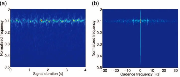
(14) wherevis the normalized frequency andh(·) is the smoothing window. The choice of the spectrogram, rather than other time-frequency distributions, is motivated by its robustness with respect to interference terms present in the so-called energy distributions [22]. An example of the spectrogram ofs(n) for a running human observed with a 16 GHz carrier frequency radar [23–25] is shown in

Fig. 3(a). The CVD, introduced in [13,26] to extract micro-Doppler features, is defined as the Fourier transform of the spectrogram along each frequency bin. An example of the CVD obtained from the spectrogram in

Fig. 3(a)is shown inFig. 3(b). The CVD provides a measure of how often the different velocities repeat (i.e., cadence frequencies) [13]. Hence, from the CVD useful information can be extracted such as the period of each of the components and their maximum micro-Doppler shifts. Specifically, all the components with a specific cadence are visible along the cadence frequency axis, while their micro-Doppler shift amplitude is visible along the normalized frequency axis. The CVD is computed as a second step of the proposed algorithm indicated inFig. 2

(ν, ε)=

K−1

k=0

χ(ν, k)e−j2π kε/K

Fig. 3. Spectrogram (a) and CVD (b) from returns relative to running man. Observation time is 4 s.

whereεis the cadence frequency.

The third step of the algorithm is the projection of the CVD onto basis constituted by the pseudo-Zernike polynomials. They depend on the CVD size only and can be precomputed through(12)and used to populate a look-up table. As the pseudo-Zernike polynomials are defined on the unit circle the CVD dimension is scaled, before the coefficient is computed, to avoid information loss. Applying(11)to(v,ε), the pseudo-Zernike expansion is obtained as

ψn,l =

n+1

π 2π

0 1

0

W_n,l∗ (ρ, θ)(ρcosθ, ρsinθ)ρdρdθ.

(16) The output of this stage is the set of (n + 1)2_magnitudes of the pseudo-Zernike coefficients; the modulus is used in order to ensure rotational invariance of the coefficients. Hence, the feature vector results are

F=|ψ0,0|, . . . ,|ψN,−N|

. (17)

Finally, the feature vectorFis normalized using the following linear rescaling

F = F−μF σF

, (18)

whereμFandσFare the mean and standard deviation of the feature vector. These values are then used to populate the micro-Doppler feature to be used as input to a classifier.

The last step of the algorithm, clearly, consists of the classification procedure. In particular, the classification has been performed using a K-nearest neighbour (KNN) classifier, to assign each element to a class, for simulated data. Moreover, on real radar data, the classification of extracted feature vectors is performed using a support vector machine (SVM) classifier with a radial basis function (RBF) kernel, employing a cross-validation grid search for selection of cost function and kernel

parameters. The one-against-all approach [27] was used to perform multiclass classification.1

III. EXPERIMENTAL RESULTS ON SIMULATED RADAR DATA

To study the behaviour of the proposed classification algorithm based on pseudo-Zernike moments, and to experimentally validate the choice of this kind of

approach, a dataset of simulated observations is considered first. Specifically, the returns from helicopter rotor blades have been simulated [6,28,29]. However, more

sophisticated and accurate models can be found in [30]. The time domain signature of rotor blades [6] is defined as

s(t)=L˜exp

−j4π

λ [R0+z0sinβ]

× NB−1

k=0

sinc (k(t)) exp{−j k(t)}

, (19)

where ˜Lis the scattering coefficient of the blade (for simplicity we consider it equal to the dimensionless length of the bladeL[5]),λis the radar operative wavelength,R0 is the distance from the radar to the origin of the reference coordinates,z0is the z-coordinate of the scattering center, βis the radar observed elevation angle,NBis the number of blades, sinc(x)=sin(x)/x, andk(t) is the phase function given by

k(t)= 4π

λ L

2cosβcos (t+φ0+k2π/N),

k=0, . . . , NB−1, (20)

withthe angular rotation rate andφ0the initial rotation angle.

Notice that the returns from helicopter rotor blades could not perfectly match with the definition of micro-Doppler, because of the corresponding high

1_{The objective of the analysis on simulated data is to show the}

Doppler shift. Consequently, terms like macro-Doppler could sound better than micro-Doppler for this case study. Nevertheless, we prefer to let the scientific community choose the more appropriate terminology.

In particular, 4 classes have been provided, each comprises 100 observations of helicopter rotor blade returns simulated using(19). Here, the parameters representing the simulated classes for a total of 400 observations are reported.

Class 1. Helicopter withNB=2 blades,L=4 m main blade length, and=10π rad/s angular rotation rate.

Class 2. Helicopter withNB=2 blades,L=6 m main blade length, and=6πrad/s angular rotation rate.

Class 3. Helicopter withNB=3 blades,L=4 m main blade length, and=10π rad/s angular rotation rate.

Class 4. Helicopter withNB=3 blades,L=6 m main blade length, and=6πrad/s angular rotation rate.

The other parameters, needed to compute(19)that are used to simulate the helicopter data, are range resolution

Rr=0.5 m, signal durationT=1 s, number of time samplesnt=10240, radar operative frequencyf0= 5 GHz, blade wideW=1 m, one end (root) of bladeL1= 0.5 m, other end (tip) of bladeL2=L + L1m, rotor center location (0,0,0), and radar location (500,0,500).

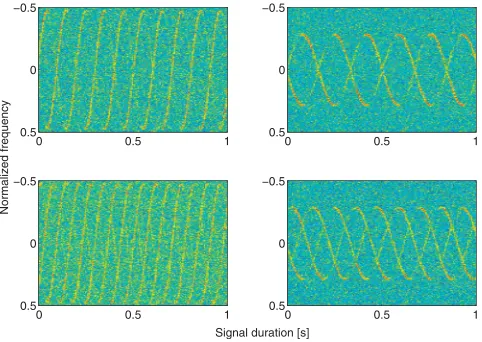
To obtain the 100 observations for each class, once the spectrogram is computed, additive zero-mean Gaussian noise has been added to it. Specifically, the spectrograms have been computed considering a number of points for the discrete Fourier transform (DFT) computationNDFT= 256, a Hamming window of lengthM=128, and with 50% overlap (notice that for the computation of the spectrogram the overlap and save method was utilized [31]).Fig. 4shows an example of a spectrogram obtained for each class and with a signal-to-noise power ratio (SNR) of 5 dB. As the figure shows, the 4 classes exhibit a different time-frequency response, representing a good test case for the proposed algorithm. Again, inFig. 5, an example of spectrogram for each class is given with an

SNR=–5 dB.

The analyses have been conducted considering 70% of data for training, while the other 30% are used for testing. In order to statistically characterize the classifier and its performance, a Monte Carlo approach has been applied, using different selections of the training and test sets of the data chosen randomly for each class. To estimate the classifier performance, 50 different experimental cases have been performed, evaluating the average correct classification (defined as the number of correct classified observations over their total number). The simulations have been performed comparing the proposed algorithm based on pseudo-Zernike moments with the one that uses the Zernike moments.

Normalized frequency

0 0.5 1

−0.5

0

0.5

0 0.5 1

−0.5

0

0.5

Signal duration [s]

0 0.5 1

−0.5

0

0.5

0 0.5 1

−0.5

0

0.5

Fig. 4. Examples of spectrogram (with SNR=5 dB) for 4 classes of returns from helicopter rotor blades. Figures on top refer to class 1 and 2,

respectively, figures on bottom refer to class 3 and 4.

Normalized frequency

0 0.5 1

−0.5

0

0.5

0 0.5 1

−0.5

0

0.5

Signal duration [s]

0 0.5 1

−0.5

0

0.5

0 0.5 1

−0.5

0

0.5

Fig. 5. Examples of spectrogram (with SNR=–5 dB) for 4 classes of returns from helicopter rotor blades. Figures on top refer to class 1 and 2

respectively, figures on bottom refer to class 3 and 4.

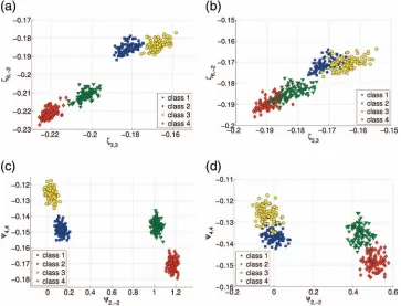
Fig. 6reports the scatter plots related to the 8th order moments of index 9 versus index 24, for all the data of the 4 classes. Note that both the Zernike and pseudo-Zernike moments have been considered. Following the rule given inTable I, it is easy to see that the above-mentioned 9th and 24th moments areζ3,3andζ6,–2for Zernike, andψ2,–2 andψ4,4for pseudo-Zernike, respectively.2The scatter plots demonstrate that for SNR=0 dB, both Zernike and pseudo-Zernike moments give a certain degree of separation within the classes. However for SNR=–5 dB the Zernike moments present a less evident separability between the elements of different classes. This behaviour is also confirmed by the results illustrated inFig. 7, where the average correct classification is plotted versus the moments order both for Zernike (dot-dashed curves) and

2_{Notice that the moments as reported in scatter plots can assume both}

Fig. 6. Scatter plot of 9th vs 24th moments of 4 helicopter rotor blades classes, for different SNR values. Figures on top refer to Zernike, figures on bottom refer to pseudo-Zernike moments both of order 8.

1 2 3 4 5 6 7 8 9 10

20 30 40 50 60 70 80 90 100

Moments Order

Correct classification [%]

SNR = −10 dB SNR = −5 dB SNR = 0 dB SNR = 5 dB

Fig. 7. Correct classification (%) versus moments order for simulated helicopter rotor blades data for different values of SNR. Solid lines represent average correct classification (over 50 runs) of algorithm based

on pseudo-Zernike moments, dot-dashed lines refer to algorithm based on Zernike moments.

pseudo-Zernike (solid curves) moments based algorithms. It is clear that, as expected, an increment in the SNR leads to higher performance; moreover, higher moments orders ensure higher percentages of correct classification, thanks to the availability of more coefficients. Finally, the curves show the different performance between Zernike and pseudo-Zernike moments based algorithms. For instance, in the case of SNR=–5 dB the 7th order pseudo-Zernike moments based algorithm reaches a correct classification

of 99.08%, while the Zernike one needs to be of order 8 to ensure the same level of correct classification. Thus, having fixed the moments order, the pseudo-Zernike framework assures a higher level of correct classification than the Zernike counterpart. Consequently, as conclusion to this analysis, it can be claimed that the use of

pseudo-Zernike moments is preferred to that of Zernike, due to their higher level of independent information at parity of order.

IV. EXPERIMENTAL RESULTS ON REAL RADAR DATA

In this section the performance of the proposed classification algorithm is assessed using real radar data. Two different dataset are used, namely, 1) the former is a Ku band radar dataset obtained in a real controlled scenario (Subsection IV-A), and 2) the latter is an X band radar dataset acquired in a more realistic environment with the target area at more than 4 km range from the radar (Subsection IV-B), both of them with an unknown level of SCR (signal-to-clutter power ratio). Moreover, this second dataset represents a good test-bench for the proposed feature due to its uncontrolled and realistic nature.

A. Experimental Results on Ku Band Radar Data

−1 −0.5 0 0.5 1 −1

−0.8 −0.6 −0.4 −0.2 0

ψ_4,−3

ψ 3,−2

class 1 class 2 class 3 class 4 class 5

Fig. 8. 5th order pseudo-Zernike momentsψ3,–2vsψ4,–3for 5 classes.

entire 4 s time observation window and on shorter time windows (2, 1, and 0.5 s), extracted from the beginning of the 4 s sequence. In this way, it is possible to test the algorithm with respect to the variation of the available observation time.

Attention has been focused on 5 different classes of data, included in the same class the case of a target moving toward and away from the radar location. A summary of the classes and acquisitions is reported below for a total of 362 acquisitions.

Class 1. Person running toward/away from the radar (284 s - 71 samples).

Class 2. Person walking toward/away from the radar (396 s - 99 samples).

Class 3. Person crawling (72 s - 18 samples). Class 4. Group of people running toward/away from

the radar (200 s - 50 samples).

Class 5. Group of people walking toward/away from the radar (496 s - 124 samples).

As used previously, from all the available samples, 70% are used for training, while the other 30% are used for testing. In order to statistically characterize the classifier and its performance, a Monte Carlo approach has been applied, using different selections of the training and test sets of the data chosen randomly for each class. To estimate the classifier performance, 50 different experimental cases have been evaluated, reporting the mean and standard deviation (or degree of reliability). The spectrogram is computed usingNDFT=512 points for the

DFT computation, and a Hamming window of lengthM=

256, with 50% overlap. Notice that the choice of the number of DFT points depends on the acquisition system [i.e., pulse repetition frequency (PRF) and the expected time dynamic of the targets (e.g. humans, animals rather than helicopters)].

Fig. 8shows the scatter plot representing the 5th order pseudo-Zernike momentsψ3,–2vsψ4,–3for all the available data. The figure shows how the objects form a quite well-defined cluster for each class that,

consequently, facilitates the separation (or classification) of the different objects. The result shown inFig. 8is confirmed by the entire analysis performed on the

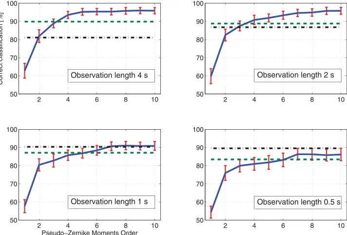
considered dataset.Fig. 9shows the average correct classification versus the pseudo-Zernike moments order for different durations of the signal, and with the corresponding degree of reliability. The average correct classification values are also summarized inTable II.

Analyzing the result ofFig. 9andTable II, it is clear that performances increase with the pseudo-Zernike moments order. In particular, it is sufficient to consider the pseudo-Zernike moments of order 5 (36 coefficients) to achieve 95% correct classification. Furthermore, as expected, as the acquisition time of the considered signals reduces, the classification performance experiences a reduction due to the reduced amount of micro-Doppler information contained in the analyzed signal [see Figs.9(a)to9(d)]. Finally, for comparison purposes, the 20-components MFP based classifier suggested in [15] and the time-frequency distribution - direction features (TFD-DF) technique proposed in [14] are considered. As the curves ofFig. 9show, the proposed classification algorithm can achieve better performance than the MFP based, if a sufficiently high moments order is chosen. The TFD-DF classifier outperforms the pseudo-Zernike based one if a 0.5 s signal length is considered; however, as the duration of the signals increases, the proposed algorithm achieves a higher probability of correct classification than the TFD-DF.

B. Experimental Results on X Band Radar Data

For a more complete analysis, the classification algorithm proposed in Section II-B was also applied to X band radar data of moving humans and animals. The dataset was generated during a single test using a Selex ES PicoSAR system operating in DMTI (dismount moving target indicator) mode (with a carrier frequency of 9.2 GHz and PRF of 2 kHz) [32]. The radar was used to target a fixed scene from a ground-based platform; in this specific scenario the SCR is low due to the extension of the observed area. Humans and/or horses were then introduced to the scene to act as targets. Data were collected for targets performing each of the following 6 classes of motion.

Class 1. Horse with rider walking (fast). Class 2. Horse with rider walking (medium). Class 3. Horse and human both present. Class 4. Human walking (fast).

Class 5. Human walking (medium). Class 6. Human walking (slow).

Fig. 9. Correct classification (%) versus pseudo-Zernike moments order. Solid line represents average correct classification (over 50 runs) with its corresponding degree of reliability, dashed curve is related to MFP based classifier proposed in [15], dot-dashed curve refers to TFD-DF classifier

given in [14]. Subplots refer to different signal lengths (i.e., 4, 2, 1, 0.5 s, respectively).

TABLE II

Average Correct Classification (%) for Different Observation Time Windows and Pseudo-Zernike Moment Orders

Pseudo-Zernike Moments Order

Observation Length [s] 1 2 3 4 5 6 7 8 9 10

4 62.8 81.8 88.8 93.5 95.2 95.3 95.3 95.7 95.9 95.8

2 59.7 82.4 87.4 90.8 91.8 93.3 94.6 94.8 95.7 95.8

1 57.6 80.4 82.7 85.7 86.8 88.4 90.6 91.0 90.8 90.8

0.5 54.3 75.9 79.9 80.9 81.7 83.1 86.2 86.2 85.7 86.1

Note:The analysis has been conducted on real Ku band radar data.

class number 3 (namely horse and human both present) represents an exception to this analysis because there are 28, 56, and 112 observations for duration of the signal 2, 1, and 0.5 s, respectively.

As already done both for simulated data and real Ku band radar data, 70% of the available data has been used for training, and the remainder 30% for testing. Again, a 50 trials Monte Carlo approach3_{has been used to} statistically characterize the proposed classification algorithm, evaluating the average correct classification and the corresponding standard deviation for each moments order and for several spectrogram configurations. Specifically, the analysis has been performed considering different settings for the spectrogram computation, to evaluate the impact of the dependency of the algorithm on the spectrogram from which the CVD and, consequently, the pseudo-Zernike moments are computed. InTable III, 4

3_{Notice that the number of Monte Carlo trials is clearly limited by the}

number of available real data.

TABLE III

Spectrogram Configurations Used for the Analyses on X Band Radar Data

Configuration Type NDFT M Overlap

a 256 256 88%

b 256 256 72%

c 256 512 70%

d 256 256 50%

combinations of the number of DFT pointsNDFT, Hamming window lengthM, and the signal’s overlap are summarized.

InFig. 10, the average correct classification is given versus the pseudo-Zernike moments order for different durations of the signal (also summarized in TablesIVand

V), and with the corresponding degree of reliability. The curves ofFig. 10and the values of TablesIVand

Vshow that for very low moments order the performances are poor, but the latter strongly increase for higher

2 4 6 8 10 40

60 80 100

2 4 6 8 10

40 60 80 100

Correct classification [%]

2 4 6 8 10

40 60 80 100

2 4 6 8 10

40 60 80 100

2 4 6 8 10

40 60 80 100

2 4 6 8 10

40 60 80 100

Pseudo−Zernike Moments Order

Observation length 2 s Observation length 2 s

Observation length 1 s

Observation length 0.5 s Observation length 0.5 s

Observation length 1 s

Fig. 10. Correct classification (%) versus pseudo-Zernike moments order. Solid line represents average correct classification (over 50 runs) with its corresponding degree of reliability, dashed curve is related to MFP based classifier proposed in [15], dot-dashed curve refers to TFD-DF classifier

given in [14]. Figures from top to bottom refer to different signal lengths (i.e., 0.5, 1, 2 s, respectively). Three figures on left are obtained from spectrograms (a), (b), and (c) ofTable III, figures on right refer to spectrogram configuration (d) ofTable III.

TABLE IV

Average Correct Classification (%) for Different Observation Time Windows and Pseudo-Zernike Moment Orders

Pseudo-Zernike Moments Order

Observation Length [s] 1 2 3 4 5 6 7 8 9 10

0.5 58.9 65.4 72.3 77.5 80.8 84.4 85.8 85.5 85.1 84.0

1 49.1 68.1 78.1 78.7 82.0 83.6 84.7 85.8 85.6 84.9

2 59.8 76.2 88.8 87.8 90.4 90.0 87.2 86.0 83.8 83.1

Note:The analysis has been conducted on real X band radar data and with the spectrogram configurations (a)-(c) ofTable III.

TABLE V

Average Correct Classification (%) for Different Observation Time Windows and Pseudo-Zernike Moment Orders

Pseudo-Zernike Moments Order

Observation Length [s] 1 2 3 4 5 6 7 8 9 10

0.5 46.9 61.7 67.2 72.8 75.7 80.1 80.1 81.0 81.4 80.9

1 46.7 63.0 72.1 76.2 78.1 80.0 82.4 84.4 83.9 82.9

2 52.4 72.4 81.4 81.5 84.2 84.1 84.3 81.5 79.3 77.2

Note:The analysis has been conducted on real X band radar data and with the spectrogram configurations (d) ofTable III.

of duration 2 s and with the spectrogram configuration (c) ofTable III, the maximum value of correct classification (90.4%) is attained with the 5th order of pseudo-Zernike moments. Thus, the analysis conducted on Ku band radar data is confirmed in the case of X band data, even if in this case the scenario utilized to acquire data is more realistic: long range, lack of clutter mitigation, and longer

wavelength are the main reasons of loss in overall

performances. Again, the classification algorithm based on pseudo-Zernike moments has been compared with the

V. CONCLUSIONS

In this paper a novel approach for micro-Doppler feature extraction has been presented. The proposed algorithm exploits the properties of the pseudo-Zernike moments to extract robust features with a limited number of values. The moments are applied to the CVD of the micro-Doppler signature in order to minimize the feature acquisition dependence. Moreover the invariant properties of the novel feature, together with the opportunity to extract a desired accuracy from the data, open to many ATR applications.

Simulated data have been used to motivate the selection of the pseudo-Zernike moments rather than the Zernike ones, besides showing good results also with uncontrolled SCR. Moreover, the novel features have been tested on real micro-Doppler data in Ku and X bands, producing high classification accuracy. The proposed approach introduces interesting elements of robustness with respect to unwanted dependencies in micro-Doppler signatures, such as translational and scale independence. These properties make the pseudo-Zernike based micro-Doppler feature potentially applicable in different scenarios, e.g. multistatic micro-Doppler ATR. Future work will involve the development of a strategy for the selection of the best order of the pseudo-Zernike moments to be used.

ACKNOWLEDGMENT

The work of C. Clemente and J. Soraghan was supported by the Engineering and Physical Research Council (Grant EP/K014307/1), the MOD University Defence Research Collaboration in Signal Processing. The authors would like to thank Selex ES Edinburgh for providing the X band data.

REFERENCES

[1] Setlur, P., Amin, M., and Ahmad, F.

Urban target classification using time-frequency micro-Doppler signatures.

International Symposium on Signal Processing and Its Applications, Sharjah, United Arab Emirates, Feb. 2007, pp. 1–4.

[2] Thayaparan, T., Abrol, S., Riseborough, E., Stankovic, L., Lamothe, D., and Duff, G.

Analysis of radar micro-Doppler signatures from experimental helicopter and human data.

IET Radar, Sonar and Navigation,1, 4 (2007), 289–299. [3] Smith, G. E., Woodbridge, K., and Baker, C. J.

Radar micro-Doppler signature classification using dynamic time warping.

IEEE Transactions on Aerospace and Electronic Systems,46, 3 (2010), 1078–1096.

[4] Chen, V. C.

Analysis of radar micro-Doppler with time-frequency transform.

InProceedings of the Tenth IEEE Workshop on Statistical Signal and Array Processing, 2000, 463–466.

[5] Chen, V. C., Li, F., Ho, S. S., and Wechsler, H.

Micro-Doppler effect in radar: Phenomenon, model, and

simulation study.

IEEE Transactions on Aerospace and Electronic Systems,42, 1 (2006), 2–21.

[6] Chen, V. C.

Micro-Doppler Effect in Radar. Boston: Artech House, 2011. [7] Clemente, C., Balleri, A., Woodbridge, K., and Soraghan, J. J.

Developments in target micro-Doppler signatures analysis: Radar imaging, ultrasound and through-the-wall radar.

EURASIP Journal on Advances in Signal Processing,47(Mar. 2013).

[8] Clemente, C., and Soraghan, J. J.

GNSS based passive bistatic radar for micro-Doppler analysis of helicopter rotor blade.

IEEE Transactions on Aerospace and Electronic Systems,50, 1 (Jan. 2014).

[9] Balleri, A., Chetty, K., and Woodbridge, K.

Classification of personnel targets by acoustic micro-Doppler signatures.

IET Radar, Sonar and Navigation,5, 9 (2011), 943–951. [10] Tahmoush, D., and Silvious, J.

Radar micro-Doppler for long range front-view gait recognition.

IEEE International Conference on Biometrics: Theory, Applications, and Systems, Washington, DC, 2009, 1–6. [11] Fogle, O. R., and Rigling, B. D.

Micro-range/micro-Doppler decomposition of human radar signatures.

IEEE Transactions on Aerospace and Electronic Systems,48, 4 (Oct. 2012), 3058–3072.

[12] Smith, G. E., Woodbridge, K., and Baker, C. J.

Template based micro-Doppler signature classification. InEuropean Radar Conference, Manchester, UK, Sept. 2006, 158–161.

[13] Bjorklund, S., Johansson, T., and Petersson, H.

Evaluation of a micro-Doppler classification method on mm-wave data.

InIEEE Radar Conference, Atlanta, GA, May 2012, 934–939.

[14] Molchanov, P., Astola, J., Egiazarian, K., and Totsky, K. Classification of ground moving radar targets by using joint time-frequency analysis.

InIEEE Radar Conference, Atlanta, GA, May 2012, 366–371.

[15] Zabalza, J., Clemente, C., Di Caterina, G., Ren, J., Soraghan, J. J., and Marshall, S.

Robust micro-Doppler classification using SVM on embedded systems.

IEEE Transactions on Aerospace and Electronic Systems, unpublished.

[16] Bhatia, A. B., and Wolf, E.

On the circle polynomials of Zernike and related orthogonal sets.

Mathematical Proceedings of the Cambridge Philosophical Society,50, 1 (1954), 40–48.

[17] Hu, M. K.

Visual pattern recognition by moment invariants.

IRE Transactions on Information Theory,8, 2 (Feb. 1962), 179–187.

[18] Teague, M.

Image analysis via the general theory of moments.

Journal of the Optical Society of America,70, 8 (Aug. 1980).

[19] Teh, C. H., and Chin, R. T.

On image analysis by the methods of moments.

IEEE Transactions on Pattern Analysis and Machine Intelligence,10, 4 (July 1988), 496–513.

[20] Bailey, R. R., and Srinath, M.

IEEE Transactions on Pattern Analysis and Machine Intelligence,18, 4 (Apr. 1996), 389–399.

[21] Khotanzad, A., and Hong, Y. H.

Invariant image recognition by Zernike moments.

IEEE Transactions on Pattern Analysis and Machine Intelligence,12, 5 (May 1990), 489–497.

[22] Cohen, L.

Time-Frequency Analysis (Signal Processing Series). Upper Saddle River, NJ: Prentice Hall, 1995.

[23] The database of radar echoes from various targets. Available: http://cid-3aaf3e18829259c0.skydrive.live.com/home. aspx.

[24] Andric, M. S., Bondzulic, B. P., and Zrnic, B. M. The database of radar echoes from various targets with spectral analysis.

Symposium on Neural Network Applications in Electrical Engineering, Belgrade, Serbia, Sept. 2010,

187–190.

[25] Andric, M. S., Bondzulic, B. P., and Zrnic, B. M.

Feature extraction related to target classification for a radar Doppler echoes.

Telecommunications Forum, 2010, 725–728. [26] Ghaleb, A., Vignaud, L., and Nicolas, J.

Micro-Doppler analysis of wheels and pedestrians in ISAR

imaging.

IET Signal Processing,2, 3 (2008), 301–311. [27] Vapnik, V. N.

Statistical Learning Theory. New York: Wiley, 1998. [28] Tait, V. N.

Introduction to Radar Target Recognition(IET Radar, Sonar and Navigation Series 18). London: IET, 2005.

[29] Stankovic, L., Djurovic, I., and Thayaparan, T.

Separation of target rigid body and micro-Doppler effects in ISAR imaging.

IEEE Transactions on Aerospace and Electronic Systems,42, 4 (Oct. 2006), 1496–1506.

[30] Martin, J., and Mulgrew, B.

Analysis of the theoretical radar return signal from aircraft propeller blades.

IEEE Radar Conference, Arlington, VA, May 1990, 569–572.

[31] Quatieri, T. F.

Discrete-Time Speech Signal Processing: Principles and Practice. Upper Saddle River, NJ: Prentice Hall, 2001. [32] Kinghorn A. M., and Nejman, A.

PicoSAR - An advanced lightweight SAR system.

European Radar Conference, Rome, Italy, Oct. 2009, 168–171.

Carmine Clemente(S ’09—M ’13) received the Laurea cum laude (B.Sc.) and Laurea Specialistica cum laude (M.Sc.) degrees in telecommunications engineering from Universita’ degli Studi del Sannio, Benevento, Italy, in 2006 and 2009, respectively. In 2012, he received the Ph.D. degree in the Department of Electronic and Electrical Engineering, University of Strathclyde, Glasgow, UK.

Currently he is a Research Associate in the Department of Electronic and Electrical Engineering, University of Strathclyde, Glasgow, U.K working on advanced radar signal processing algorithm, MIMO radar systems, and micro-Doppler analysis. His research interests include synthetic aperture radar (SAR) focusing and bistatic SAR focusing algorithms development, micro-Doppler signature analysis and extraction from multistatic radar platforms, micro-Doppler classification, and statistical signal processing.

Luca Pallotta(S’12) received the Laurea Specialistica degree (cum laude) in telecommunication engineering in 2009 from the University of Sannio, Benevento, Italy, and the Ph.D. degree in electronic and telecommunication engineering in 2014 from the University of Naples Federico II, Naples, Italy.

His research interest lies in the field of statistical signal processing, with emphasis on radar signal processing and radar targets classification.

Antonio De Maio(S’01—A’02—M’03—SM’07—F’13) was born in Sorrento, Italy, on June 20, 1974. He received the Dr.Eng. degree (with honors) and the Ph.D. degree in information engineering, both from the University of Naples Federico II, Naples, Italy, in 1998 and 2002, respectively.

From Oct. to Dec. 2004, he was a visiting researcher with the U.S. Air Force Research Laboratory, Rome, NY. From Nov. to Dec. 2007, he was a visiting researcher with the Chinese University of Hong Kong, Hong Kong. Currently, he is an Associate Professor with the University of Naples Federico II. His research interest lies in the field of statistical signal processing, with emphasis on radar detection, optimization theory applied to radar signal processing, and multiple-access communications.

Dr. De Maio is the recipient of the 2010 IEEE Fred Nathanson Memorial Award as the young (less than 40 years of age) AESS Radar Engineer 2010 whose performance is particularly noteworthy as evidenced by contributions to the radar art over a period of several years.

John J. Soraghan(S ’83—M ’84—SM ’96) received the B.Eng. (Hons.) and M.Eng.Sc. degrees in electronic engineering from University College Dublin, Dublin, Ireland, in 1978 and 1983, respectively, and the Ph.D. degree in electronic engineering from the University of Southampton, U.K., in 1989.

After graduating, he worked with the Electricity Supply Board in Ireland and with Westinghouse Electric Corporation in the United States. In 1986, he joined the Department of Electronic and Electrical Engineering, University of Strathclyde, Glasgow, U.K., as a Lecturer and became a Senior Lecturer in 1990, a Reader in 2000, and a Professor in Signal Processing in September 2003, within the Institute for Communications and Signal Processing (ICSP). In Dec. 2005, he became the Head of the ICSP. He currently holds the Texas Instruments Chair in Signal Processing with the University of Strathclyde. He was a Manager of the Scottish Transputer Centre from 1988 to 1991, and a Manager of the DTI Parallel Signal Processing Centre from 1991 to 1995. His main research interests are signal processing theories, algorithms and architectures with applications to remote sensing, telecommunications, biomedicine, and condition monitoring.

Prof. Soraghan is a member of the IET.

Alfonso Farina(M’95—SM’98—F’00) received the doctor degree in electronic engineering from the University of Rome (I), Italy, in 1973.

In 1974, he joined Selenia, now SELEX Electronic Systems, where he has been a Manager since May 1988. He was Scientific Director in the Chief Technical Office. He was the Director of the Analysis of Integrated Systems Unit. He was also the Director of Engineering in the Large Business Systems Division. In 2012, he was the Chief Technology Officer of the Company (SELEX Sistemi Integrati). Today he is Senior Advisor to CTO of SELEX ES. In his

Dr. Farina is the author of more than 500 peer-reviewed technical publications and the author of books and monographs:Radar Data Processing(Vol. 1 and 2) (translated into Russian and Chinese), (Researches Studies Press, and Wiley, 1985-1986);

Optimized Radar Processors, (on behalf of IEE, Peter Peregrinus, 1987); andAntenna Based Signal Processing Techniques for Radar Systems, 1992. He wrote the chapter “ECCM Techniques” in theRadar Handbook(2nd ed., 1990, and 3rd ed., 2008), edited by Dr. M. I. Skolnik (NRL, USA). Dr. Farina has been session chairman at many international radar conferences. In addition to lecturing at universities and research centers in Italy and abroad, he also frequently gives tutorials at the International Radar Conferences on signal, data, and image processing for radar; in particular on