Quantitative data graphics in 3D desktop-based virtual environments – an evaluation

City, University of London Institutional Repository

Citation

: Dykes, J. and Bleisch, S. (2015). Quantitative data graphics in 3D

This is the accepted version of the paper.

This version of the publication may differ from the final published

version.

Permanent repository link:

Link to published version

: http://dx.doi.org/10.1080/17538947.2014.927536

Copyright and reuse:

City Research Online aims to make research

outputs of City, University of London available to a wider audience.

Copyright and Moral Rights remain with the author(s) and/or copyright

holders. URLs from City Research Online may be freely distributed and

linked to.

Pre-proof copy: Bleisch, S., & Dykes, J. (2014). Quantitative data graphics in 3D desktop-based virtual environments – an evaluation. International Journal of Digital Earth, 1–17. doi:10.1080/17538947.2014.927536

Quantitative data graphics in 3D desktop-based virtual environments - an

evaluation

Susanne Bleisch1 _{and Jason Dykes}2

1_{Geomatics Engineering, FHNW University of Applied Sciences and Arts Northwestern Switzerland,}

Muttenz, Switzerland; 2_{giCentre, City University London, London, UK}

3D desktop-based virtual environments provide a means for displaying quantitative data in context. Data that is inherently spatial in three-dimensions may benefit from visual exploration and analysis in relation to the environment in which they were collected and to which they relate. We empirically evaluate how effectively and efficiently such data can be visually analyzed in relation to location and landform in 3D versus 2D visualizations. In two experiments, participants performed visual analysis tasks in 2D and 3D visualizations and reported insights and their confidence in them. The results showed only small differences between the 2D and 3D visualizations in the performance measures that we evaluated: task completion time, confidence, complexity, and insight plausibility. However, we found differences for different data sets and settings suggesting that 3D visualizations, or 2D representations respectively, may be more or less useful for particular data sets and contexts.

Keywords: 3D, geovisualization, quantitative data graphics, visual data analysis, empirical evaluation

Introduction

Geovisual analytics considers spatial characteristics as an important dimension in making sense of data (Andrienko et al. 2010). Thus, data that are inherently spatial in three-dimensions may benefit from being visually explored and analyzed in the context of the landscape or other three-dimensional aspects of the environment to which they relate. Earlier research (Bleisch, Dykes, and Nebiker 2008; Bleisch 2011) has shown some potential for displaying quantitative data as data graphics in 3D desktop-based virtual environments. The study presented here evaluated the performance of this 3D geovisualization technique for visual data analysis by integrating the results from two experiments employing quantitative data graphics with different data sets and tasks.

Background

Research aim

As Shepherd (2008, 200) notes, we may need to overcome the “3D for 3D’s sake” tendency and consider when 3D is more appropriate than 2D in particular contexts. One such case could be when the data to be analyzed has a clear relation to the dimensional landscape in which it was collected. As this case has inherent three-dimensional spatial properties we may make use of a three-three-dimensional representation even though we are less effective at analyzing the depth dimension than the up-down or sideways dimensions of three-dimensional representations (Ware 2008). Any deficiencies may be mitigated by the ability to change viewpoint in 3D, perhaps at the cost of time spent making such changes. This study aims to help us better understand how well three-dimensional representations perform in comparison to more traditional 2D representations, with a particular emphasis on such three-dimensional patterns and relationships. The evaluation presented here is based on a comparison of quantitative and qualitative analytical task performance measures between different data sets (and the environment to which they relate) displayed in 2D representations and 3D desktop-based virtual environments. These conditions are termed `2D' and `3D' subsequently. North (2006) claims that insight is the purpose of visualization. Consequently, the study described here follows North’s (2006) definition of qualitative, complex, and relevant insights for the qualitative task performance measures. We hypothesize that 3D representations facilitate data analysis in relation to the 3D landform and vice versa 2D representations facilitate data analysis in relation to location. Specifically, we want to evaluate whether exploratory data analysis tasks that have a direct reference to either location (a 2D concept) or altitude (including landforms and height differences) are more efficiently (time) and effectively (confidence, complexity and plausibility) solved in the 2D or 3D representations respectively.

Evaluation methods

We planned and conducted two experiments to evaluate the usefulness of data graphics in 3D desktop-based virtual environments - E1 and E2. The experiments used data sets and tasks of varying complexity to compare participants' task performance between the 2D and 3D environments. The data in both experiments were displayed as single bars (univariate data) or bar charts (multivariate data) without (2D environment) or with reference frames (3D environment) following earlier experimental results (Bleisch et al. 2008). To facilitate broad participation at different spatial locations both experiments were administered through online questionnaires that could be completed remotely.

Visual analysis tasks

The definition of tasks is a complex issue in geovisualization evaluations (Tobon 2005). Interaction taxonomies (e.g., Yi et al. 2007) often combine navigation, data display manipulation, and analysis tasks. For 3D visualizations, which are interactive by nature, it is helpful to separate between the different types as we did not test or control for navigation tasks but focused solely on analysis. Additionally, the hypotheses stated required task definitions in which exploration and data analysis were performed in relation to the surrounding landscape - specifically those in which location and altitude/landform were considered with the source data either independently or in combination. Frequently used data analysis tasks include identify, compare, or categorize as defined in task taxonomies by Wehrend and Lewis (1990) or Zhou and Feiner (1998). However, they do not intuitively support specific definitions of references for the analysis of data, which were core to the current hypotheses. The alternative functional view of data and tasks (Andrienko and Andrienko 2006) allows analysis tasks to be defined in terms of two components of data: characteristic and reference. Thus, tasks either referring to location and/or altitude could be defined. Additionally, the Andrienko and Andrienko (2006) task framework allows a wide range of tasks to be defined at different levels of complexity (elementary and synoptic) as is relevant to data exploration. This framework was thus used in our experiments to define directed exploratory tasks to facilitate ideation (Marsh 2007).

Experiment E1

each of two 2D representations and two 3D representations. The seven tasks (Table 1) used were of varying complexity (elementary and synoptic) and had different reference sets (Andrienko and Andrienko 2006). Two tasks referred to location, three tasks referred to altitude and two tasks referred to location and altitude in combination (Table 1). The visualizations were arranged in a balanced order in the different questionnaires to counter confounding carry-over effects such as familiarization with a setting, getting used to the tasks or tiredness occurring towards the end of a series of several tasks. The questionnaires contained instructions, a test task to ensure Google Earth was installed on the system and that JavaScript was enabled, in addition to the different visualizations and tasks. They were implemented to be completed online with a current web browser. The questionnaires connected to a database and in total 932 insight reports were collected – 468 in the 2D condition, 464 in 3D. On average each participant spent 45 minutes on the questionnaire, including reading the instructions, testing the installations and completing the seven tasks in each of two 2D and two 3D representations.

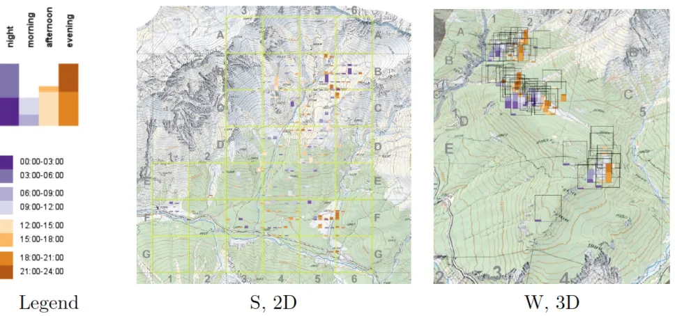
Experiment E2

Experiment E2 extends experiment E1 to multivariate data displays in virtual environments. Two data sets consisting of the aggregated four summer and four winter data sets from experiment E1 were used to prepare four visualizations in 3D and 2D. Once again we used Google Earth for the 3D condition and HTML, SVG and JavaScript for the 2D condition. Both conditions allowed interaction such as zooming and panning, and viewpoint change was available in the 3D case (Figure 2). Data analysis showed that the seven tasks used in E1 strongly influenced the participants in their analysis as indicated, for example, by their use of words in the reported insights that were similar to those used in describing the task. Thus, experiment E2 employed one synoptic exploratory task (referring to location, altitude and time of the day, cf. Table 1, task E2.1) in which participants were asked to report all insights gained from visually analyzing the data (Rester et al. 2007) and thus resulting in a less guided data exploration session. In a within-subject design, 38 informed participants reported insights and judged their confidence in each insight when visually analyzing one 2D and one 3D representation. Participants were final year Geomatics students – from a different but comparable cohort to those who had participated in E1. The representations, together with experiment instructions and a test task to ensure that Google Earth and JavaScript were working, were implemented as online questionnaires that could be completed in a web browser. Once again, the questionnaires contained the representations in a balanced order to counter confounding factors. The questionnaires connected to a database and in total 522 insights were collected – 260 in the 2D case and 262 in the 3D case. On average each participant spent 50 minutes completing the questionnaire, including reading the instructions, testing installations and working on the task with the two data sets and representations.

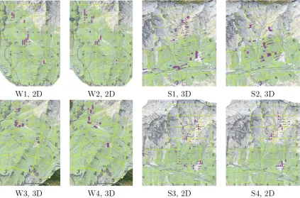
The data used for the different settings in E1 and E2 were different subsets and aggregations of tracking data associated with a single deer (eight different settings in E1, cf. Figure 1, and two different settings in E2, cf. Figure 2). To account for the influence of different topographies on the analysis, the subset of the data collected during the winter months was spatially shifted to a nearby area that is also frequented by roaming deer. These settings are labeled `W' (winter) in Figures 1 and 2, with settings in which the deer data are displayed in their original environment labeled `S' (summer). This procedure could have resulted in the loss of some of the connection the deer tracks have with the environment. However, this influence is likely to be minimal as the area into which the data was shifted is also frequented by deer and their movements are generally more limited during wintertime.

Figure 2: Quantitative data and map background (1:25000 © 2014 swisstopo (BA14010)) of the two different settings (W and S) either in 2D (HTML, SVG and JavaScript) or 3D (Google Earth)

Data analysis

# task reference(s) E1.1 Which area is most often visited by the deer? location (L) E1.2 Which altitude/altitude range is most often visited by the deer? altitude (A) E1.3 Generally, compare the number and distribution of deer visits in

the lower areas to the number of deer visits in higher areas?

altitude (A)

E1.4 Compare the location and altitude of areas with similar deer visit patterns?

location & altitude (LA) E1.5 In which area(s) does the number of deer visits increase with

increasing altitude?

location & altitude (LA) E1.6 Describe the deer visit patterns in relation to altitude and

landform (surface / topographic features and undulations.

altitude (A)

E1.7 Describe the deer visit patterns in relation to location and land-cover?

location (L)

E2.1 Analyze the deer data and describe the deer habits regarding location, altitude and time of the day.

location & altitude (LA)

Table 1. Directed exploratory tasks for experiment E1 (tasks E1.1 - E1.7) and experiment E2 (task E2.1) referring either to location (L) or altitude (A) or a combination of location and altitude (LA).

category (label) subcategory example words

location (L) datum D3, F4 (grid squares)

(L) object forest, scree, grassy

(L) relation/description north, left, south-east

altitude (A) datum 1950m, 2400m

(A) object mountain, slope, ridge

(A) relation/description steep, lower, highest

Table 2. Word categories used to classify an answer/insight into either referring to location, altitude or a combination of both.

Results

Comparing performance measures between 2D and 3D

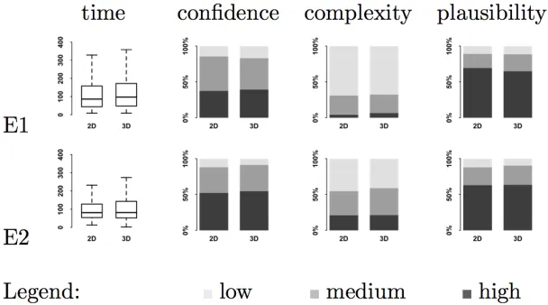
Overall, comparing task times, confidence ratings, complexity and plausibility measures between the 2D and 3D representations in both experiments E1 and E2 did not reveal any significant difference between the 2D and 3D settings (Figure 3).

Comparing performance measures between reference sets

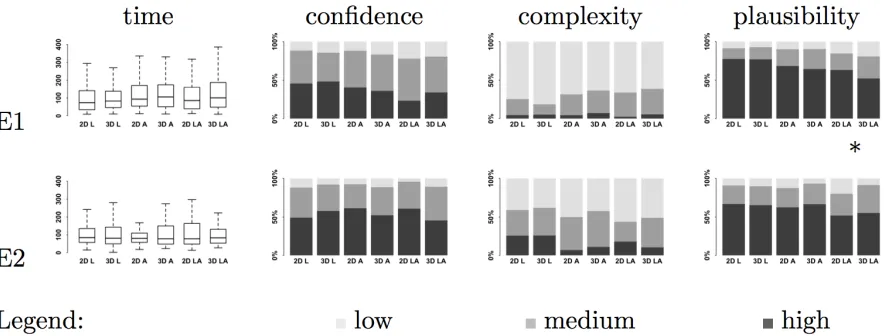
Each task in E1, as well as each collected insight report in E1 and E2, had its own reference set. It referred either to altitude (A), location (L) or a combination of both (LA) based on the terms used in describing the task (see Data Analysis section). Thus we were able to compare times, confidence ratings, complexity and plausibility measures for different reference sets and to evaluate our hypotheses that the 3D representation facilitates tasks relating to altitude and that 2D representations facilitate tasks referring to location. The data analysis showed a statistically significant difference (at level 95%) in E1 for the plausibility ratings with the LA reference set (combination of location and altitude) between 2D and 3D (marked with * in Figure 4). The insights reported from the LA reference set in 3D were less often of high plausibility but more frequently of medium or low plausibility than in the 2D case. However, none of the other performance measure comparisons revealed a statistically significant difference between the different reference sets (Figure 4). Overall, neither the 3D nor the 2D representations seemed to either facilitate or hinder data exploration in either the 2D or the 3D representation.

Figure 4: Comparison of the performance measures time, confidence, complexity and plausibility (columns) between the different reference sets of the insights in 2D and 3D for the experiments E1 and E2 (rows).

Generally, no statistically significant differences (at significance level 95%) were found between 2D and 3D for the different reference sets. The only statistically significant difference was in E1 for plausibility ratings with reference set LA (combination of location and altitude) between 2D and 3D (marked *) (X2=6.09, df = 2, p-value = 0.048).

Comparing performance measures between experiments

Figures 3 and 4 show some differences and trends when comparing the two experiments E1 and E2. For example, participants were significantly more confident when reporting insights based on one generic task in E2 than reporting on the seven more specific tasks in E1 (2D: X2=14.72, df=2, p-value=0.001; 3D: X2=18.53, df=2, p-value<0.001). Additionally, the synoptic task in E2 led to significantly more complex insights being reported (2D: X2_{=93.74, df=2, p-value<0.001; 3D: X}2_{=79.56, df=2, p-value<0.001). Experiment E1 used seven tasks}

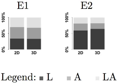
Figure 5: Comparison of relative quantities of

reference set usage (location L, altitude A or both LA) in the insights reported in E1 and E2.

Figure 6: Comparison of relative quantities of

reference set usage (location L, altitude A or both LA) in the insights reported in E1 compared to the task references (tasks referring to location tL, tasks referring to altitude tA and tasks referring to a combination of location and altitude tLA).

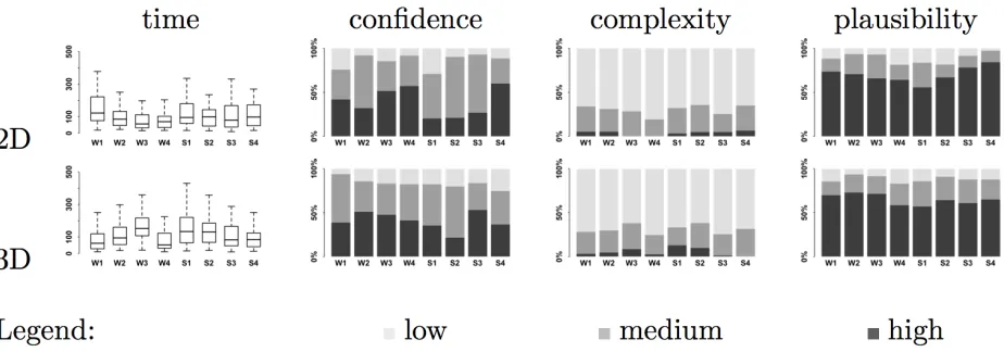
Comparing performance measures for different settings

All the settings in E1 and E2 used similar data - different subsets and aggregations of tracking data recorded by a single animal, as described in the Evaluation Methods section. However, comparing time, confidence, complexity and plausibility measures between the settings for E1 and E2 (Figure 7) showed that there were some significant differences between 2D and 3D. The summer setting in E1 is a case in point, where more time was required in 3D than 2D (Z=-2.01, p-value=0.044) and more insights of high plausibility were yielded in 2D than 3D (X2_{=8.27, df=2, p-value=0.016). The winter setting in E2 also revealed differences between the 2D and}

3D conditions as participants were more confident about the findings reported in the 3D case compared to 2D (X2_{=10.57, df=2, p-value=0.005).}

Figure 7: Comparing the performance measures time, confidence, complexity and plausibility for the different settings (W and S) between 2D and 3D.

Looking for trends in the eight different data sets in E1 we found differences between 2D and 3D for the task performance measures for most data sets (Figure 8). Small number of results in a few categories prevented statistical testing for significance as the research was not originally set up to detect differences in analysis between settings and data sets. Nevertheless, summarizing the trends in Figure 8 it seems that some settings and data sets may be better analyzed either in 2D or 3D or using a combination of both representation types. In the case of just one setting and data set (W2) analysis in 2D or 3D seem to be equally successful with regard to the evaluated performance measures.

Setting W2: The results for time, confidence, complexity and plausibility were similar for the 2D and 3D conditions in setting W2. We conclude that setting W2 is equally successfully analyzed either in 2D or 3D.

Setting W3: Insights were reported more quickly and with less variation in completion time in 2D. The results for confidence and plausibility were similar for 2D and 3D. However, the 3D setting shows a trend for a higher number of insights of high and medium complexity. We conclude that setting W3 is analyzed more rapidly in 2D but may yield more complex insights in the 3D setting.

Setting W4: Reporting time, complexity and plausibility of insights in setting W4 were similar for 2D and 3D with some trends such as 3D being slightly quicker but yielding fewer highly plausible insights. Participants were more confident in their reported insights in 2D. We conclude that setting W4 may best be analyzed using a combination of 2D and 3D representations.

Setting S1: Setting S1 was analyzed more quickly in 2D but with more confidence in the 3D case. A trend towards more complex insights in 3D was apparent. Plausibility was similar for 2D and 3D. We conclude that setting S1 may be analyzed most effectively using a combination of 2D and 3D representations.

Setting S2: Insights were reported more quickly in 2D. The results for confidence, complexity and plausibility were similar for 2D and 3D. We conclude that setting S2 is analyzed more rapidly in 2D.

Setting S3: The results showed similar analysis times and complexity for 2D and 3D. However, insights were reported with more confidence in 3D but higher plausibility in 2D. We conclude that setting S3 may best be analyzed using a combination of 2D and 3D representations.

Setting S4: The results of setting S4 showed less variation in insight reporting times in 3D. However, insights were reported with higher confidence, complexity and plausibility in 2D. We conclude that setting S4 may be more successfully analyzed in 2D than 3D.

These trends may suggest that analysis in 2D, 3D or a combination of both types of representation may be preferable dependent on the data and setting. Only setting W2 seems to be analyzed with comparable levels of success in either representation type. Relating these preferences back to specific characteristics of the settings, such as topography, and data sets (number, range and distribution of the data values) used in these experiments proved difficult. We found no clear relationship between setting characteristics and improved performance in terms of the analysis of the data in one representation type or the other. However, this data dependent finding draws attention to the fact that open designs, in which a variety of options for display and interaction can be accessed quickly and smoothly, may well be important. We are however unable to make predictions based upon data characteristics as yet. In the context of Andrienko et al.’s recommendation that we “develop appropriate design rules and guidelines for interactive displays of spatial and temporal information” (Andrienko et al. 2010, 1596) the guideline here given current knowledge may be to emphasize flexible and responsive interactions through which alternative representations can be accessed rather than data and context invariant rules for visual design. This is achievable in the kinds of dynamic environments used in geovisual analytics.

We note that differences between the settings would be expected. All seven tasks could not be equally well completed with all of the data sets. However, this does not explain the differences between 2D and 3D as the same tasks were attempted with the same data set using the 2D and 3D visualizations.

Discussion and conclusions

In our two experiments a total of 72 different informed participants were able to work with the two types of representations (2D and 3D) to visually analyze the data sets based on different directed exploratory tasks (Table 1). 1,454 insights, mostly of high plausibility, were collected. Consequently, we conclude that 2D bars or bar charts with reference frames on billboards are a viable option for displaying quantitative data in desktop-based 3D virtual environments for elementary and synoptic tasks in a range of settings. Participants were able to work with the displays and report insights based on exploratory tasks. This confirms earlier findings developed in more controlled settings (Bleisch et al. 2008; Bleisch 2011) and suggests that these apply to use cases involving more complex data sets and tasks. Some evidence suggests that participants found analysis of data in relation to landform difficult even though they were able to do so. We may need to improve tools to help them if we deem these kinds of tasks to be important.

For more detailed understanding, especially of the potential of three-dimensional representations (as suggested by MacEachren and Kraak 2001), we then analyzed the data predominantly for differences between the two representation types - 2D and 3D. However, contrary to our expectation, we found no significant difference between the two types of representation for the evaluated performance measures (time, confidence, complexity and plausibility) either in experiment E1 or E2. Additionally, analyzing the data for different reference sets (location, altitude or both) required us to reject our initial hypotheses: we found no evidence that the 3D display of the landform and setting either helps or hinders the interpretation of altitude differences and landform through our experiments; similarly, the 2D display of landform and setting neither helps nor hinders the interpretation of positional aspects such as spatial distribution. However, the analysis of comments, participants reporting more insights in relation to location in E2 as well as the lower confidence ratings for altitude related tasks in E1 indicate that visual analysis of quantitative data sets in relation to altitude and landform is not common. The fact that our participants were not used to analyzing data in relation to the landform may somewhat confound the results of this study. However, for the comparison between 2D and 3D this influence is minimized through the within-subject design, where participants were asked to perform exactly the same tasks with both representation types.

Generally, conclusions from empirical evaluations are somewhat limited to the data sets used in testing, the particular interface developed and the group of participants used. We sought informed users as participants in our experiments. 72 students and staff from different universities and different ‘geo’-subjects ensured that the experiments were conducted with a large group of users that has interest in these types of interfaces and analysis tasks. Still, the results pertain to this user group and broad generalizations may need further research.

evaluated by Bleisch and Nebiker (2008), and commonly used in multi-view 2D information visualization interfaces (Keim 2002), could be helpful. Once again, further evaluation is needed.

The empirical data presented here shows that in our particular context no significant difference between visual data analysis using either 2D or 3D representations was found. However, importantly there was a variation in results depending on data sets and settings. It suggests that future research in this area should focus on when (in terms of data characteristics and settings) 3D geovisualizations are more or less useful than other types of representations and supporting means of establishing this exploration with appropriate environments for visual analysis rather than more general comparisons of 2D versus 3D.

Acknowledgements

The authors thank the Swiss Nationalpark, especially Dr. Ruedi Haller, for providing the deer data. The background map data of the experiments is reproduced with authorization of swisstopo (map data 1:25000 © 2014 swisstopo (BA14010)). We are very grateful to the participants for taking part in the experiments, investing their time and thus facilitating this research. The authors also thank the two anonymous reviewers for their valuable comments and suggestions, which have been used to improve this article.

References

Andrienko, G., Andrienko, N., Demsar, U., Dransch, D., Dykes, J., Fabrikant, S. I., Jern, M., Kraak, M.-J., Schumann, H., and Tominski, C. 2010. "Space, time and visual analytics." International Journal of Geographical Information Science, 24 (10): 1577–1600.

Andrienko, N., and Andrienko, G. 2006. Exploratory Analysis of Spatial and Temporal Data: A Systematic Approach. Berlin: Springer.

Bartoschek, T., and Schönig, J. 2008. "Trends und Potenziale von virtuellen Globen in Schule, Lehramtsausbildung und Wissenschaft." GIS.Science, 2008 (4): 28–31.

Bleisch, S. 2011. "Towards appropriate representations of quantitative data in virtual environments."

Cartographica, 46 (4): 252–261. doi:10.3138/carto.46.4.252.

Bleisch, S., Dykes, J., and Nebiker, S. 2008. "Evaluating the Effectiveness of Representing Numeric Information Through Abstract Graphics in 3D Desktop Virtual Environments." The Cartographic Journal, 45 (3): 216–226. doi:10.1179/000870408X311404.

Bleisch, S., and Nebiker, S. 2008. "Connected 2D and 3D visualizations for the interactive exploration of spatial information." Paper presented at the XXIst ISPRS Congress, Beijing, China, July 3-11.

Butler, D. 2006. "Virtual globes: the web-wide world." Nature, 439 (7078): 776–778.

Gleicher, M., Albers, D., Walker, R., Jusufi, I., Hansen, C. D., and Roberts, J. C. 2011. "Visual comparison for information visualization." Information Visualization, 10 (4): 289–309. doi:10.1177/1473871611416549. Keim, D. A. 2002. "Information Visualization and Visual Data Mining." IEEE Transactions on Visualization

and Computer Graphics, 7 (1): 100–107.

Lam, H., Bertini, E., Isenberg, P., Plaisant, C., and Carpendale, S. 2011. "Empirical Studies in Information Visualization: Seven Scenarios." IEEE Transactions on Visualization and Computer Graphics, 18 (9): 1520– 1536. doi:10.1109/TVCG.2011.279.

MacEachren, A. M., and Kraak, M.-J. 2001. "Research Challenges in Geovisualization." Cartography and Geographic Information Science, 28 (1): 3–12.

Marsh, S. L. 2007. "Using and Evaluating HCI Techniques in Geovisualization: Applying Standard and Adapted Methods in Research and Education." PhD diss., City University London.

Neuendorf, K. A. 2002. The Content Analysis Guidebook. Thousand Oaks: Sage Publications, Inc.

North, C. 2006. "Toward Measuring Visualization Insight." IEEE Computer Graphics and Applications, 26 (3): 6–9.

Patterson, T. C. 2007. "Google Earth as a (Not Just) Geography Education Tool." Journal of Geography, 106 (4): 145–152.

Rester, M., Pohl, M., Wiltner, S., Hinum, K., Miksch, S., Popow, C., and Ohmann, S. 2007. "Evaluating an InfoVis Technique Using Insight Reports." In Information Visualization, 2007, 11th _{International Conference}

Sandvik, B. 2008. "Using KML for Thematic Mapping." MSc thesis, University of Edinburgh.

Sedlmair, M., Ruhland, K., Hennecke, F., Butz, A., Bioletti, S., and O’Sullivan, C. 2009. "Towards the Big Picture  : Enriching 3D Models with Information Visualisation and Vice Versa." In Proceeding SG ’09 Proceedings of the 10th International Symposium on Smart Graphics, edited by A. Butz, 27–39. Berlin Heidelberg: Springer-Verlag.

Seipel, S., and Carvalho, L. 2012. "Solving Combined Geospatial Tasks Using 2D and 3D Bar Charts." In 2012 16th International Conference on Information Visualisation, 157–163. IEEE. doi:10.1109/IV.2012.36.

Shepherd, I. D. H. 2008. "Travails in the Third Dimension  : A Critical Evaluation of Three-dimensional Geographical Visualization." In Geographic Visualization: Concepts, Tools, and Applications, edited by M. Dodge, M. McDerby and M. Turner, 199–222. Chichester: John Wiley & Sons Ltd.

Slingsby, A., Dykes, J., and Wood, J. 2008. "A Guide to Getting your Data into Google Earth." Accessed April 14. http://www.willisresearchnetwork.com/Lists/WRN News/Attachments/8/An introduction to Getting your Data in Google Earth2.pdf

Slocum, T. A., McMaster, R. B., Kessler, F. C., and Howard, H. H. 2009. Thematic cartography and geovisualization. 3rd ed. Upper Saddle River: Pearson Prentice Hall.

Tobon, C. 2005. "Evaluating Geographic Visualization Tools and Methods: An Approach and Experiment Based upon User Tasks." In Exploring Geovisualization, edited by J. Dykes, A. M. MacEachren and M.-J. Kraak, 645–666. Oxford: Elsevier.

Ware, C. 2008. Visual Thinking for Design. Burlington: Elsevier Inc.

Ware, C., and Plumlee, M. 2005. "3D Geovisualization and the Structure of Visual Space." In Exploring Geovisualization, edited by J. Dykes, A. M. MacEachren and M.-J. Kraak, 567–576. Oxford: Elsevier.

Wehrend, S., and Lewis, C. 1990. "A Problem-oriented Classification of Visualization Techniques." In

Proceedings of the First IEEE Conference on Visualization, Visualization '90, 139–143. San Francisco: IEEE. Wood, J., Dykes, J., Slingsby, A., and Clarke, K. 2007. "Interactive Visual Exploration of a Large Spatio-Temporal Dataset: Reflections on a Geovisualization Mashup." IEEE Transactions on Visualization and Computer Graphics, 13 (6): 1176–1183.

Yi, J. S., Kang, Y., Stasko, J. T., and Jacko, J. A. 2007. "Toward a Deeper Understanding of the Role of Interaction in Information Visualization." IEEE Transactions on Visualization and Computer Graphics, 13 (6): 1224–1231.