City, University of London Institutional Repository
Citation
:
Fairbank, M., Prokhorov, D. and Alonso, E. (2013). Approximating Optimal
Control with Value Gradient Learning. In: Lewis, F. and Liu, D. (Eds.), Reinforcement
Learning and Approximate Dynamic Programming for Feedback Control. (pp. 142-161).
Hoboken, NJ, USA: Wiley-IEEE Press. ISBN 111810420X
This is the accepted version of the paper.
This version of the publication may differ from the final published
version.
Permanent repository link:
http://openaccess.city.ac.uk/5192/
Link to published version
:
http://dx.doi.org/10.1002/9781118453988
Copyright and reuse:
City Research Online aims to make research
outputs of City, University of London available to a wider audience.
Copyright and Moral Rights remain with the author(s) and/or copyright
holders. URLs from City Research Online may be freely distributed and
linked to.
CHAPTER 7
APPROXIMATING OPTIMAL CONTROL
WITH VALUE GRADIENT LEARNING
Michael Fairbank1, Danil Prokhorov2 and Eduardo Alonso1
1City University London, London, UK 2
Toyota Research Institute NA, Ann Arbor, Michigan
Abstract
In this chapter we extend the ADP algorithm, Dual Heuristic Programming (DHP), to
include a “bootstrapping” parameterλ, analogous to that used in the Reinforcement
Learning algorithm TD(λ). The resulting algorithm, which we call VGL(λ) for
value-gradient learning, is proven to produce a weight update that can be equivalent to
backpropagation through time (BPTT) applied to a greedy policy on a critic-function.
This provides a surprising connection between the two alternative methods of BPTT
approximator for the critic. We show that this can lead to increased stability in the
learning of control problems by a neural network.
7.1 INTRODUCTION
Adaptive Dynamic Programming (ADP) is the study of how an agent can learn actions
that maximise a long-term reward [13]. For example a typical scenario is an agent
wandering around in an environment, such that at timetit has state vector~xt. At
each timetthe agent chooses an action~atwhich takes it to the next state according to
the environment’s (possible stochastic) model function~xt+1 =f(~xt, ~at), and gives
it an immediate scalar rewardrt, given by the reward functionrt =r(~xt, ~at). The
agent keeps moving, forming a trajectory of states(~x0, ~x1, . . .), which terminates if and when a designated terminal state is reached. The ADP problem is for the agent
to learn how to choose actions so as to maximise the expectation of the total reward
received,hP
tγ tr
ti, whereγ∈[0,1]is a constantdiscount factorthat specifies the
importance of long term rewards over short term ones. Specifically, the problem
is to find a policy functionπ(~x, ~z), where~z is the parameter vector of a function approximator, that calculates which action~a=π(~x, ~z)to take for any given state~x, such that this total reward sum is maximised.
In this chapter we concentrate on the sub-problem of when the model functions
f(~x, ~a)andr(~x, ~a)are comprised of a twice-differentiable deterministic part, plus optionally some additive noise. We assume that these functions are unchanging
and either already known analytically, or already learned beforehand by a system
identification process, for example by using a neural network as described by [17].
One paradigm of ADP is to learn avalue function,V(~x), from Bellman’s Opti-mality Principle [1], and then choose a policy function that is “greedy” on that value
function. A greedy policy is one that always chooses actions which lead to states with
the highestV value (whilst also taking into account the immediate short-term reward
in getting there). These methods use an approximated function (e.g. the output of a
neural network) to represent the learnedV function, and this approximated function
meth-INTRODUCTION 3
ods include Heuristic Dual Programming, Dual Heuristic Programming (DHP) and
Globalized Dual Heuristic Programming (GDHP) from the ADP literature [13, 16, 9],
and TD(λ) and Q-learning from the reinforcement learning (RL) literature [11, 14].
Critic learning methods can be very effective and computationally efficient, but
proving their convergence when a general function approximator is used for V is
challenging, and even more challenging when combined with a greedy policy.
One reason that convergence analysis is difficult with a greedy policy is that in
the Bellman condition,V depends on the policyπ, which, being greedy, depends on
V; so making progress in learning one of them can undo progress in learning the
other. We make an important insight into this difficulty by showing (in Lemma 4)
that the dependency of a greedy policy on a value function is through what we call the
value-gradient, which we define to be ∂V∂~x. Hence a value-gradient analysis seems necessary at some level to provide a theoretical gateway to analysing the convergence
properties of any critic weight update that uses a greedy policy in a continuous state
space. We refer to algorithms that specifically aim to learn the value-gradient ∂V∂~x as “value-gradient learning” (VGL) algorithms. The existing ADP algorithms DHP
and GDHP are examples of value-gradient learning algorithms.
We extend the DHP and GDHP algorithms into a new algorithm that we call
VGL(λ). This extension algorithm includes a constant parameterλ∈[0,1]analogous to that used in TD(λ), such that VGL(0) is equivalent to DHP. The motivation for
doing this extension is similar for the motivation for using TD(λ) in preference to
TD(0): By choosingλcarefully we might get faster and more stable learning.
An alternative paradigm of ADP is to use backpropagation through time (BPTT,
[15]), which is gradient ascent on the total long term reward with respect to the
policy’s parameter vector~z. Since this is gradient ascent on a function that is bound
above, proving convergence is more straightforward.
In this chapter we demonstrate a theoretical connection between these two
para-digms of ADP (i.e. between critic learning and BPTT). We prove that, under certain
strict conditions, doing BPTT on a greedy policy function is equivalent to VGL(1)
with a carefully chosen learning parameter, “Ωt”, described below. This proof of
guarantees of BPTT will also apply to this critic learning method, with a greedy
policy, and a general function approximator forV. Hence we provide a convergence
proof for this instance of the algorithm in this chapter.
The convergence proof requires a particular choice of a learning parameter matrix,
Ωt. This was defined by Werbos for the algorithm GDHP (e.g. see [18, eq. 32]).
Previously there was little guidance on how to set this matrix, but our proof and
discussions (in sections 7.3.4 and 7.4.3) cast some new light on this problem.
Other convergence proofs do exist for critic learning methods, but they do not
generally apply to a greedy policy or a critic function implemented by a general
function approximator. For example the RL algorithm TD(λ) [11] has been proven
to converge [12] provided the function approximator forV is linear in its parameter
vector, and the policy is fixed (i.e. that excludes the greedy policy). This particular
algorithm is not proven to converge when a general function approximator is used
to represent the critic (e.g. a neural network) or when a greedy policy is used.
Divergence examples exist for a non-linear function approximator [12], and where
the function approximator forV is linear in its weight vector but where a greedy
policy is used (diverging for bothλ= 0andλ= 1; see [6]). A convergence proof for general critic learning was given by [8], although this assumed the critic function
being used could always be made to exactly learn any given target values, and so this
is not realistic for a general function approximator. In the case of a general function
approximator and a greedy policy, popular ADP methods such as DHP and GDHP
can also be forced to diverge [6].
The structure of this chapter is as follows: We define the VGL(λ) and BPTT
algorithms in section 7.2. We prove their equivalence in section 7.3, and discuss
the conditions for convergence in section 7.3.3, and insights into theΩtmatrix in
sections 7.3.4 and 7.4.3. In section 7.4 we define a simple computer experiment and
demonstrate the improved convergence properties of the VGL algorithm over DHP.
We also define an efficient form for the greedy policy andΩtmatrix in section 7.4.2.
VALUE GRADIENT LEARNING AND BPTT ALGORITHMS 5
7.2 VALUE GRADIENT LEARNING AND BPTT ALGORITHMS
First we give some preliminary definitions and notation, and then follow with the
algorithm definitions.
7.2.1 Preliminary Definitions
Critic function: We defineVe(~x, ~w)to be the scalar output of a smooth function approximator with weight vector w~. This can also be known as theapproximate value function.
Critic gradient function:We define the critic gradient function to beGe(~x, ~w)≡
∂Ve(~x, ~w)
∂~x . The VGL and DHP algorithms attempt to learn this quantity. The critic
gradient can also be known as theapproximate value gradient.
Smooth policy function: We define a general smooth policy functionπ(~x, ~z)to be the output of a smooth function approximator with output vector of dimension
dim(~a), and with parameter vector~z. This is also referred to in the literature as an “action network” or “actor”.
Approximate Q function:We define the functionQe(~x, ~a, ~w)to be
e
Q(~x, ~a, ~w) =r(~x, ~a) +γVe(f(~x, ~a), ~w) (7.1)
This function comes up often in this chapter in the greedy policy and its related
lemmas. It is related to, but not identical to, the Q-function defined by [14].
Matrix and vector notation used: We make a notational convention that all
vectors are columns, and differentiation of a scalar by a vector gives a column vector.
So for exampleGe,~xand ∂∂~Vex are all columns. We define differentiation of a vector function by a vector as follows:1 ∂Ge
∂ ~wis a matrix with element(i, j)equal to
∂Ge(~x, ~w)j
∂ ~wi .
Similarly, ∂f∂~xis the matrix with element∂f∂~x
ij
= ∂f∂~(~x,~xia)j.
Trajectory Shorthand Notation: All subscripted “t” indices refer to the
time-step of a trajectory and provide corresponding arguments~xtand~atwhere appropriate;
so that for exampleVet+1≡Ve(~xt+1, ~w),rt≡r(~xt, ~at),Get≡Ge(~xt, ~w)and
∂ e
Q ∂~a
t
is shorthand for the function∂Qe(~x,~a, ~w)
∂~a evaluated at(~xt, ~at, ~w). Similarly
∂Ge
∂ ~w
t
≡
∂Ge
∂ ~w
(~x
t, ~w)
.
7.2.2 VGL(λ) Algorithm
The VGL algorithm is an extension of the DHP algorithm [16] to include a constant
parameterλanalogous to that used in the algorithm TD(λ). The algorithm requires
the derivatives off(~x, ~a),r(~x, ~a),π(~x, ~z)andVe(~x, ~w)all to exist at every time-step along a trajectory.
Using the notation conventions of section 7.2.1, and the implied matrix products,
the VGL(λ) algorithm is defined to be a critic weight update of the form:
∆w~ =αX
t
∂Ge
∂ ~w
!
t
Ωt(G0t−Get) (7.2)
whereαis a small positive constant;Ωt ∈ <dim(~x)×dim(~x)is an arbitrary positive
definite matrix described further below;Getis the critic gradient; andG0tis the “target
value gradient” defined recursively by:
G0t=
Dr
D~x
t
+γ
Df
D~x
t
λG0t+1+ (1−λ)Get+1
(7.3)
withG0t =~0at any terminal state, and whereλ ∈ [0,1]is a fixed constant; and
whereD~Dxis shorthand for D D~x≡
∂ ∂~x+
∂π ∂~x
∂
∂~a; (7.4)
and where all of these derivatives are assumed to exist. We ensure the recursion in
equation 7.3 converges by requiring that eitherγλ <1, or the environment is such that the agent is guaranteed to reach a terminal state at some finite time (i.e. the
environment is “episodic”).
Equations 7.2, 7.3 and 7.4 define the VGL(λ) algorithm. These equations can be
implemented by unrolling a whole trajectory and then working backwards along it
applying the recursion of equation 7.3, as demonstrated in pseudocode of Algorithm
7.1, which runs in timeO(dim(w~))per trajectory step. Alternatively, it is possible to apply the weight update in an on-line manner as described by [7, Appendix B], but
VALUE GRADIENT LEARNING AND BPTT ALGORITHMS 7
When we choose the parameterλ= 0, then we get the VGL(0) algorithm which is equivalent to DHP. Like DHP, the objective of the VGL(λ) weight update is to make
the valuesGetmove towards the target valuesG0t.
Ωtwas introduced by [18, eq. 32] for the GDHP algorithm, and is included in our
weight update for full generality. This positive definite matrix can be set as required
by the experimenter since its presence ensures every component ofGet will move
towards the corresponding component ofG0t(in any basis). However choosing what
value to use forΩtis not obvious, so it is often just taken to be the identity matrix
for allt. We make an insight into how to chooseΩtby finding an explicit formula
for it in section 7.3.2.
Algorithm 7.1
VGL(λ) algorithm {
t←0, ∆w~←~0
while not terminated(~xt)
~
at←π(~xt, ~z)
~
xt+1←f(~xt, ~at)
t←t+ 1
end while
F ←t
~ p←~0
for t=F−1 to 0 step −1
G0
t←
Dr D~x
t+γ
Df D~x
t~p
∆w~←∆w~+
∂Ge
∂ ~w
tΩt
G0t−Get
~ p←λG0
t+ (1−λ)Get
end for
~
w←w~+α∆w~
}
policy function weight update, i.e.
∆~z=βX
t
∂π
∂~z
t
∂r
∂~a
t
+γ
∂f
∂~a
t
e
Gt+1
. (7.5)
whereβis a separate learning rate for the policy function.
There are a variety of schemes to do this concurrently with the critic training. For
example, the policy could be trained to completion in between every critic function
weight update (a process known as value-iteration), or the vice-versa arrangement
could be applied (a process known as policy-iteration). Or a simple concurrent
scheme of doing alternating iterations of each could be applied. A final option is to
use a greedy policy function, as described in section 7.3.1, which obviates the need
for training the policy, and can be viewed as an extreme form of value-iteration.
In Algorithm 7.1, the critic functionGe(~x, ~w)can be interpreted aseithera synonym for ∂Ve(~x, ~w)
∂~x , which implies that ∂Ge
∂ ~w ≡ ∂2Ve
∂ ~w∂~x, or alternatively Ge(~x, ~w)could be implemented more simply as the output of a smooth vector function approximator of
dimensiondim(~x). We call the first of these two options a “GDHP-style critic” and the second a “DHP-style critic”. A GDHP-style critic is the harder of the two options
to implement, since it requires second order backpropagation to find ∂Ge
∂ ~w, while a
DHP-style critic only requires first-order backpropagation for this quantity. In the
experiments of section 7.4.4 we use a DHP-style critic, for simplicity.
7.2.3 BPTT Algorithm
We defineR(~x0, ~z)to be the total discounted reward encountered by an agent starting at state~x0and then following a policyπ(~x, ~z)until termination, so thatR(~x0, ~z) = P
tγ tr
t. This function can be witten recursively as:
R(~x, ~z) =r(~x, π(~x, ~z)) +γR(f(~x, π(~x, ~z)), ~z) (7.6)
withR(~x, ~z) = 0at any terminal state.
BPTT is gradient ascent onR(~x0, ~z)with respect to~z, i.e. ∆~z =β ∂R∂~z
0for some small positive constantβ. Expanding the term ∂R∂~z
tgives:
∂R
∂~z
t
= ∂
∂~z(r(~x, π(~x, ~z)) +γR(f(~x, π(~x, ~z)), ~z))
t
A CONVERGENCE PROOF FOR VGL(1) FOR CONTROL WITH FUNCTION APPROXIMATION 9 = ∂π ∂~z t ∂r ∂~a t +γ ∂f ∂~a t ∂R ∂~x t+1 ! +γ ∂R ∂~z t+1
where we used the chain rule, trajectory shorthand notation,~at = π(~xt, ~z) and
~
xt+1=f(~xt, ~at). Expanding this recursion gives:
∂R
∂~z
0 =X
t≥0
γt ∂π ∂~z t ∂r ∂~a t +γ ∂f ∂~a t ∂R ∂~x t+1 !
It is common practice to drop theγtfactor in this equation. Combining this with
the gradient ascent equation,∆~z=β ∂R∂~z
0, gives the BPTT weight update:
∆~z=βX
t≥0 ∂π ∂~z t ∂r ∂~a t +γ ∂f ∂~a t ∂R ∂~x t+1 ! (7.7)
This equation is the BPTT weight update. It refers to the quantity ∂R∂~x which can be found recursively by differentiating equation 7.6 and using the chain rule, giving
∂R ∂~x t = Dr D~x t +γ Df D~x t ∂R ∂~x t+1 (7.8)
with∂R∂~x =~0at any terminal state.
Equation 7.8 can be understood to be backpropagating the quantity ∂R∂~xt+1 through the actor network, model and reward functions to obtain ∂R∂~x
t, and giving
the algorithm its name.
7.3 A CONVERGENCE PROOF FOR VGL(1) FOR CONTROL WITH
FUNCTION APPROXIMATION
In this section we define an equivalence proof between VGL(1) and BPTT applied to
a greedy policy. Since BPTT is gradient ascent on a function that is bound above, it
has relatively good convergence guarantees, and hence the equivalence proof can be
used to make a convergence guarantee for VGL(1).
First we describe the greedy policy with some useful lemmas, then we prove the
equivalence of BPTT to VGL(1), and then discuss the convergence conditions. For the
equivalence and convergence to hold we require a specifically chosen time-dependent
7.3.1 Using a Greedy Policy with a Critic function
The greedy policy is defined to choose actions as follows:
~a= arg max
~
a∈<n(Qe(~x, ~a, ~w)) ∀~x (7.9)
whereQe(~x, ~a, ~w)is defined in equation 7.1.
For VGL, we required all of the constituent functions of equation 7.1 to be smooth,
therefore under this requirement,Qe is a smooth function with respect to all of its
parameters.
The greedy policy depends onVe(~x, ~w), i.e. uses the weight vectorw~ instead of
~
z. This means the greedy policy is a function π(~x, ~w)(instead of the usual policy dependencyπ(~x, ~z)). Hence from now on, when considering the greedy policy, it is thesameweight vectorw~that controls the policy as is used for the critic function, and so we will writeπ(~x, ~w)to always specifically mean thegreedypolicy. Any change to the critic function will immediately affect the greedy policy and move trajectories,
and we need to take this into account when proving convergence.
Greedy Actions:A greedy action is one that satisfies equation 7.9.
Since a greedy action selects amaximumwith respect to~aof the smooth function e
Q(~x, ~a, ~w), the following two consequences hold:
Lemma 1 For a greedy action~a,∂Qe
∂~a =~0.
Lemma 2 For a greedy action~a, ∂2Qe
∂~a∂~a is a negative semi-definite matrix.
Furthermore, we prove three less obvious lemmas about greedy actions and a
greedy policy:
Lemma 3 The greedy policy implies ∂~∂ra
t=−γ
∂f
∂~a
t
e
Gt+1.
Proof: First, we note that differentiating equation 7.1 gives
∂Qe
∂~a
!
t
= ∂r
∂~a
t
+γ
∂f
∂~a
t
e
Gt+1 (7.10)
A CONVERGENCE PROOF FOR VGL(1) FOR CONTROL WITH FUNCTION APPROXIMATION 11
Lemma 4 When ∂ ~∂πw
t and
∂2
e
Q ∂~a∂~a
−1
t
exist for an action~at, the greedy policy
implies
∂π
∂ ~w
t
=−γ ∂Ge ∂ ~w
! t+1 ∂f ∂~a T t ∂2 e Q ∂~a∂~a
!−1
t
Proof:We use implicit differentiation. The dependency of~at=π(x~t, ~w)onw~ must
be such that Lemma 1 is always satisfied, since the policy is greedy. This means
that∂Qe
∂~a
t≡
~0, both before and after any infinitesimal change tow~. Therefore the
functionπ(~xt, ~w)must be such that,
~0 = ∂ ∂ ~w
∂Qe(~xt, π(~xt, ~w), ~w)
∂~at
!
= ∂ ∂ ~w
∂Qe(~xt, ~at, ~w)
∂~at
! +
∂π
∂ ~w
t
∂ ∂~at
∂Qe(~xt, ~at, ~w)
∂~at
!
= ∂ ∂ ~w
∂r ∂~a t +γ ∂f ∂~a t e
Gt+1
+
∂π ∂ ~w
t
∂2Qe
∂~a∂~a
!
t
= ∂ ∂ ~w
∂r
∂~a
t
+γX
i
∂(f)i
∂~a
t
(Get+1)i !
+ ∂π
∂ ~w
t ∂2 e Q ∂~a∂~a ! t
=γX
i
∂(f)i ∂~a
t
∂(Get+1)i
∂ ~w +
∂π ∂ ~w
t
∂2Qe
∂~a∂~a
!
t
=γ ∂Ge ∂ ~w
! t+1 ∂f ∂~a T t + ∂π
∂ ~w
t ∂2 e Q ∂~a∂~a ! t
In the above six lines of algebra, line 2 is by the chain rule and substitution of
~at=π(~xt, ~w); line 3 is by equation 7.10; line 4 just expands an inner product; line
5 follows since ∂r∂~a and ∂f∂~a are not functions of w~; and line 6 just forms an inner product.
Then solving the final line for ∂ ~∂πw
tproves the lemma.
Lemma 5 When ∂π∂~xt and ∂2Qe
∂~a∂~a
−1
t exist for an action~at, the greedy policy
implies
∂π
∂~x
t
=−γ ∂
2 e Q ∂~x∂~a ! t ∂2 e Q ∂~a∂~a
!−1
This lemma is useful because it provides the quantity ∂π∂~xtwhich is used in the VGL(λ) algorithm definition, in equation 7.4. This enables us to use the VGL(λ)
algorithm with agreedypolicy.
Proof: The proof is virtually the same as that of Lemma 4, but with the start point
changed to~0 = ∂~∂x∂Qe(x~t,π(~xt, ~w), ~w)
∂~at
.
7.3.2 The Equivalence of VGL(1) to BPTT
BPTT can be defined on any smooth policy function π(~x, ~z). A greedy policy, π(~x, ~w), can be defined on anycritic function Ge(~x, ~w). In this section we apply BPTT to thegreedypolicy functionπ(~x, ~w), and we observe the resulting combined weight update that emerges. Surprisingly, we find that this weight update is identical
to the VGL(1) weight update, provided theΩtmatrix is chosen carefully. This proves
that the VGL(λ) weight update of equation 7.2, withλ= 1and a carefully chosen Ωtmatrix, is equivalent to BPTT on a greedy policy.
First we note that by comparing equations 7.3 and 7.8, we see that
G0t≡
∂R
∂~x
t
whenλ= 1 (7.11)
The BPTT gradient ascent weight update, following on from equation 7.7, but
now using a greedy policyπ(~x, ~w)instead of a general policy functionπ(~x, ~z), is
∆w~=βX
t≥0
∂π ∂ ~w
t ∂r ∂~a t +γ ∂f ∂~a t ∂R ∂~x t+1 ! (eq. 7.7) =βX
t≥0
∂π ∂ ~w
t γ ∂f ∂~a t
−Get+1+ ∂R ∂~x t+1 !
by Lemma 3 =βX
t≥0
γ
∂π ∂ ~w
t ∂f ∂~a t
G0t+1−Get+1
by eq. 7.11 =βX
t≥0
−γ2 ∂Ge ∂ ~w
! t+1 ∂f ∂~a T t
∂2Qe
∂~a∂~a
!−1 t ∂f ∂~a t
(G0t+1−Get+1) by Lemma 4
=βX
t≥0
γ2 ∂Ge ∂ ~w
!
t
A CONVERGENCE PROOF FOR VGL(1) FOR CONTROL WITH FUNCTION APPROXIMATION 13
where
Ωt=
−∂f∂~a
T t−1
∂2
e
Q ∂~a∂~a
−1
t−1 ∂f
∂~a
t−1 if
t >0
0 ift= 0
, (7.13)
and is positive semi-definite, by the greedy policy (Lemma 2).
Equation 7.12 is identical to a VGL weight update equation (eq. 7.2), with a
carefully chosen matrix forΩt, andλ= 1, provided ∂ ~∂πw
tand
∂2
e
Q ∂~a∂~a
−1
t exist for
allt. If ∂ ~∂πwtdoes not exist, then ∂R∂ ~wis not defined either.
This completes the demonstration of the equivalence of a critic learning algorithm
(VGL(1), with the conditions stated above) to BPTT on a greedy policyπ(~x, ~w) (wherew~ is the weight vector of a critic functionGe(~x, ~w)defined for Algorithm 7.1), when ∂R∂ ~wexists.
7.3.3 Convergence conditions
Good convergence conditions exist for BPTT since it is gradient ascent on a function
that is bound above, and therefore convergence is guaranteed if that surface is smooth
and the learning step size is sufficiently small. If the ADP problem is such that
∂π
∂ ~w always exists, and we chooseΩtby equation 7.13, then the above equivalence
proof shows that the good convergence guarantees of BPTT will apply to VGL(1).
Significantly∂ ~∂πwalways does exist in a continuous time setting when a value-gradient policy using the technique of section 7.4.2 is used.
In addition to smoothness of the policy, we also require smoothness of the
func-tions,randf, for VGL to be defined; and also for the convergence of BPTT that
we have proved equivalence to, the weight vector for the policy must only traverse
smooth regions of the surface ofR(~x, ~w).
If all of these conditions are satisfied, then this approximated-critic value-iteration
scheme will converge.
This has been a non-trivial accomplishment in proving convergence for a smoothly
approximated critic function with a greedy policy, even though it is only proven for
λ= 1. Other related algorithms withλ= 1, such as TD(1) and Sarsa(1), and VGL(1)
conditions when a greedy policy is used [6]. Algorithms withλ= 0, such as TD(0), Sarsa(0), DHP and GDHP are also shown to diverge with a greedy policy by [6].
While the smoothness of all functions is required for provable convergence, in
practice a sufficient condition appears to be piece-wise continuity, as BPTT has been
applied successfully to systems with friction and dead-zones.
7.3.4 Notes on the
Ω
tmatrixTheΩtmatrix that we derived in equation 7.13 differs from the previous instances of
its use in the literature (e.g. [18, eq. 32]):
• Firstly, ourΩt matrix is time dependent, whereas previous usages of it have
not used atsubscript.
• Secondly, we have found an exact equation on how to choose it (i.e. equation
7.13). Previous guidance on how to choose it has been only intuitive.
• Thirdly, equation 7.13 often only produces a positiveindefinitematrix which is problematic for the case ofλ <1. If we havedim(~x)>dim(~a)then the matrix ∂f∂~a will be wider than it is tall, and so the matrix product in equation 7.13 will yield anΩtmatrix that is rank deficient (i.e. positive indefinite). It
seems that it is not a problem to have a rank-deficientΩtmatrix whenλ= 1
(as section 7.3.2 effectively proves), but it is a problem when λ < 1. A rank-deficientΩtmatrix will have some zero eigenvalues, and the components
ofGecorresponding to these missing eigenvalues will not be learned at all by
equation7.2. However in the case ofλ <1, the definition ofG0tin equation 7.3
depends upon potentiallyallof the components ofGet+1via the multiplication in equation 7.3 by
Df D~x
t. So if some of the components of
e
Gt+1are missing, then the target gradientsG0twill be wrong, and so the VGL(λ) algorithm will
be badly defined.
This view that it is necessary forΩtto be full-rank forλ <1is consistent with
the original positive-definite requirement made by Werbos for GDHP, which
VERTICAL LANDER EXPERIMENT 15
Consequently, our choice ofΩtmatrix is best used for the situation ofλ= 1and
a greedy policy. But we feel it may provide some guidance in how to chooseΩtin
other situations, especially if working in a problem wheredim(~x)≤dim(~a). And even if the policy is not greedy, then equation 7.13 might still be a usefulguiding
choice forΩt, since it is the objective of the training algorithm for the actor network
to always try to make the policy greedy.
The Ωt matrix definition in equation 7.13 requires an inverse of the following
rather cumbersome looking matrix:
∂2Qe
∂~a∂~a
! t =∂ ∂~a ∂r ∂~a t +γ ∂f ∂~a t e
Gt+1
by eq. 7.10
⇒ ∂ 2
e
Q ∂~ai∂~aj
!
t
=
∂2r ∂~ai∂~aj
t
+γ
∂2f ∂~ai∂~aj
t
e
Gt+1+γ
∂f ∂~ai
t
∂Ge
∂~x
!
t+1
∂f ∂~aj
T
t
(7.14)
Hence to evaluate theΩtmatrix, we could require knowledge of the functions,
f andr, so that the first and second order derivatives in equations 7.13 and 7.14
could be manually computed. Computing equation 7.13 is no more challenging to
implement than computing∂π∂~xby Lemma 5, which is a necessary step to implement the VGL(λ) algorithm with a greedy policy. In many cases, such as in section 7.4.2,
both of these computations simplify considerably, for example if the functions are
linear in~a, or in a continuous time situation. Alternatively, if a neural network is
used to represent the functionsfandr, then we would require first and second order
backpropagation through the neural network work to find these necessary derivatives.
We make further observations on the role of theΩtmatrix in section 7.4.3.
7.4 VERTICAL LANDER EXPERIMENT
We describe a simple computer experiment which shows VGL learning with a greedy
policy and demonstrates increased learning stability of VGL(1) compared to DHP
(VGL(0)). We also demonstrate the value of using the Ωt matrix as defined by
equation 7.13 which can make learning progress achieve consistent convergence to
After defining the problem in section 7.4.1, we derive an efficient formula for the
greedy policy andΩtmatrix (section 7.4.2), which provides some further insights into
the purpose ofΩt(section 7.4.3), before giving the experimental results in section
7.4.4.
7.4.1 Problem Definition
A spacecraft is dropped in a uniform gravitational field, and its objective is to make
a fuel-efficient gentle landing. The spacecraft is constrained to move in a vertical
line, and a single thruster is available to make upward accelerations. The state vector
~
x= (h, v, u)Thas three components: height (h), velocity (v), and fuel remaining (u).
The action vector is one-dimensional (so that~a ≡a∈ <) producing accelerations a ∈ [0,1]. The Euler method with time-step ∆t is used to integrate the motion, giving functions:
f((h, v, u)T, a) =(h+v∆t, v+ (a−kg)∆t, u−(ku)a∆t)T
r((h, v, u)T, a) =−(kf)a∆t+rc(a)∆t (7.15)
Here,kg= 0.2is a constant giving the acceleration due to gravity; the spacecraft
can produce greater acceleration than that due to gravity.kf = 1is a constant giving
fuel penalty. ku = 1is a unit conversion constant. ∆twas chosen to be 1. rc(a)
is an “action cost” function described further below that ensures the greedy policy
function chooses actions satisfyinga∈[0,1].
Trajectories terminate as soon as the spacecraft hits the ground (h= 0) or runs out of fuel (u= 0). For correct gradient calculations, clipping is needed at the terminal time-step, and differentiation of the functions needs to take account of this clipping.
Further details of clipping are given by [5, Appendix E.1].
In addition to the reward functionr(~x, a)defined above, a final impulse of reward equal to−1
2mv
2−m(k
g)his given as soon as the lander reaches a terminal state,
wherem= 2is the mass of the spacecraft. The terms in this final reward are cost terms for the kinetic and potential energy respectively. The first cost term penalises
landing too quickly. The second term is a cost term equivalent to the kinetic energy
VERTICAL LANDER EXPERIMENT 17
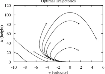
A sample of ten optimal trajectories in state space is shown in figure 7.1.
0 20 40 60 80 100 120
-10 -8 -6 -4 -2 0 2 4 6
h
(height)
[image:18.595.178.354.132.256.2]v(velocity) Optimal Trajectories
Figure 7.1 State space view of a sample of optimal trajectories in the Vertical Lander problem. Each trajectory starts at the cross symbol, and ends ath= 0. Theu-dimension (fuel) of state space is not shown.
For the action cost function, we follow the method of [3], and choose
rc(a) =−
Z
g−1(a)da (7.16)
whereg(x)is a chosen sigmoid function, as this will forcea to be bound to the range of the chosen functiong(x), as illustrated in the following subsection. Hence to ensurea∈[0,1], we use
g(x) =1
2(tanh(x/c) + 1) (7.17)
wherec= 0.2is a sharpness constant, and therefore
rc(a) =c
aarctanh(1−2a)−1
2ln(2−2a)
.
7.4.2 Efficient evaluation of the greedy policy
The greedy policyπ(~x, ~w)is defined to choose the maximum with respect to~aof the
e
Q(~x, ~a, ~w)function. This function has been defined to be smooth, so a numerical solver could be used to maximise this function, while introducing some inefficiency.
that asw~ or~xchange, the global maximum could hop from one local maximum to
another, meaning the derivatives∂π∂~xand∂ ~∂πwwould not be defined in these instances. We can get around these problems, and derive a closed form solution to the greedy
policy, by following the method of [3]. This leads to a very efficient and practical
solution to using a greedy policy, and avoids the need to use an actor network
altogether. To achieve this though, we do have to transfer to a continuous time
analysis, i.e. we consider the case in the limit of∆t → 0. The most important benefit that this delivers is that it forces the greedy policy function to be always
differentiable, and hence for the VGL(λ) algorithm to be always defined.
We make a first order Taylor series expansion of theQe(~x, ~a, ~w)function (eq. 7.1) about the point~x:
e
Q(~x, ~a, ~w)≈r(~x, ~a) +γ
∂Ve
∂~x
!T
(f(~x, ~a)−x~) +Ve(~x, ~w)
=r(~x, ~a) +γGe(~x, ~w) T
(f(~x, ~a)−~x) +γVe(~x, ~w) (7.18)
This approximation becomes exact in continuous time. We next define a greedy
policy that maximises equation 7.18. Differentiating equation 7.18 gives
∂Qe
∂a
!
t
= ∂r
∂a
t
+γ
∂f
∂a
t
e
Gt by eq. 7.18
=−(kf)∆t+
∂rc(a)∆t
∂a
t
+γ∆t(0,1,−1)Get by eq. 7.15
=−(kf)−g−1(at) +γ(0,1,−1)Get
∆t by eq. 7.16 (7.19)
For the greedy policy to satisfy equation 7.9, we must have∂Qe
∂a = 0. Therefore,
0 =−(kf)−g−1(at) +γ(0,1,−1)Get by eq. 7.19
⇒at=g
−(kf) +γ(0,1,−1)Get
(7.20)
This closed form greedy policy is efficient to calculate, bound to[0,1], and most importantly, always differentiable. This has achieved the objectives we aimed for by
moving to continuous time. Furthermore, we get a simplified expression for theΩt
VERTICAL LANDER EXPERIMENT 19
Sincedim(~a) = 1, ∂2Qe
∂a∂ais a scalar:
∂2Qe
∂a∂a
!
t
=
∂−(kf)−g−1(at) +γ(0,1,−1)Get
∂at
∆t by eq. 7.19
=−∂g −1(a
t)
∂at
∆t
=− 1 g0(g−1(a
t))
∆t differentiating an inverse
=− 1 g0−(k
f) +γ(0,1,−1)Get
∆t by eq. 7.20
(7.21)
Here g0 is the derivative of the sigmoidal function g given by equation 7.17.
Substituting equation 7.21 into equation 7.13 gives,
Ωt= (0,1,−1)Tg0
−(kf) +γ(0,1,−1)Get
(0,1,−1)∆t (7.22)
This is a much simpler version of theΩtmatrix than that described by equations
7.13 and 7.14. The simplicity arose because of the linearity with respect toaof the
functionf(x, a)and because of the change to continuous time.
Since we have moved to continuous time for the sake of deriving this efficient and
always differentiable greedy policy, there are some consequential minor changes that
we should make to the VGL algorithm. Firstly, if we were to re-derive lemmas 3,
4 and 5 using theQefunction of equation 7.18, then the references in the lemmas to
e
Gt+1would change toGet. For example, Lemma 4 would change to:
∂π
∂ ~w
t
=−γ ∂Ge ∂ ~w
!
t
∂f
∂~a
T
t
∂2 e
Q ∂~a∂~a
!−1
t
(7.23)
The VGL(λ) weight update would be the same as equation 7.12, but we would use
Ωtas given by equation 7.22, and the greedy policy given by equation 7.20. Also ∂π∂~x
(which is needed in the VGL(λ) algorithm in equation 7.4) is found most easily by
differentiating equation 7.20, as opposed to using Lemma 5.
We note that equation 7.23, when combined with equation 7.21, is consistent with
7.4.3 Observations on the purpose of
Ω
tNow that we have a simple expression forΩt, we can make some observations on
its purpose. SubstitutingΩtof equation 7.22 into the VGL weight update (eq. 7.2)
gives:
∆w~ =αγ2(∆t)X
t≥0
∂Ge
∂ ~w
!
t
(0,1,−1)Tg0−(kf) +γ(0,1,−1)Get
(0,1,−1)(G0t−Get)
(7.24)
This has similarities in form to a weight update for the supervised learning neural
network problem. Consider a neural network output functiony =g(s(~x, ~w))with sigmoidal activation function g, summation function s(~x, ~w), input vector ~xand weight vectorw~. To make the neural network learn targetstpfor input vectors~xp
(wherepis a “pattern” index), the gradient descent weight update would be:
∆w~ =αX
p
∂yp
∂ ~w(tp−yp)
=αX
p
∂s(~xp, ~w)
∂ ~w g 0(s(~x
p, ~w)) (tp−yp) (7.25)
The similarities in equations 7.24 and 7.25 give hints at the purpose ofΩt, since
it is theΩtmatrix that introduces theg0 term into the VGL weight update equation
(eq. 7.24). In neural network training, we would not omit theg0term from a weight
update, and we would not treat it as a constant; and likewise we deduce that we
should not omit theΩt matrix or treat it as fixed in the VGL learning algorithm.
In neural network training, some algorithms choose to give theg0 term an artificial
boost to help escape plateaus of the error surface in weight space (e.g. Fahlman’s
method [4] which replacesg0byg0+k, for a small constantk), but this comes at the expense of the learning algorithm no longer being true gradient descent, and hence
it not being as stable. Choosing to setΩt ≡ I, the identity matrix, is like doing
an extreme version of Fahlman’s method on the VGL algorithm. This can help the
learning algorithm escape plateaus of theRsurface very effectively, but may lead to
divergence. Plateaus are a severe problem whencis small in equation 7.17, since
VERTICAL LANDER EXPERIMENT 21
Having made these deductions about the role ofΩtin VGL, we should make the
caveat that these deductions only strictly apply to VGL(1) with a greedy policy, as
that is the algorithm thatΩtwas derived for.
7.4.4 Experimental Results for Vertical Lander Problem
A DHP-style critic,Ge(~x, ~w), was provided by a fully connected multi-layer percep-tron (MLP) (see [2] for details). The MLP had 3 inputs, two hidden layers of 6
units each, and 3 units in the output layer. Additional short-cut connections were
present fully connecting all pairs of layers. The weights were initially randomised
uniformly in the range[−1,1]. The activation functions were logistic sigmoid func-tions in the hidden layers, and a linear function with slope 0.1 in the output layer.
The input to the MLP was a rescaling of the state vector, given by D(h, u, v)T,
whereD=diag(0.01,0.1,0.02), and the output of the MLP gaveGedirectly. In our implementation, we also defined the functionf(~x, ~a)to input and output coordinates rescaled byD, the intention being to ensure that the value gradients would be more
appropriately scaled too.
Three algorithms were tested: VGL(0) withΩt=I, the identity matrix; VGL(1)
withΩt=I; and VGL(1) withΩtgiven by equation 7.13 (denoted by throughout by
“VGLΩ(1)”). Each algorithm was set the task of learning a group of 10 trajectories
with randomly chosen fixed start points (the 10 start points used in all experiments
are those shown in figure 7.1), and with initial fuelu= 30. In each iteration of the learning algorithm, the weight update was first accumulated for all 10 trajectories,
and then this aggregate weight update was applied. In some experiments RPROP
was used to accelerate this aggregate weight update at each iteration, with its default
parameters defined by [10].
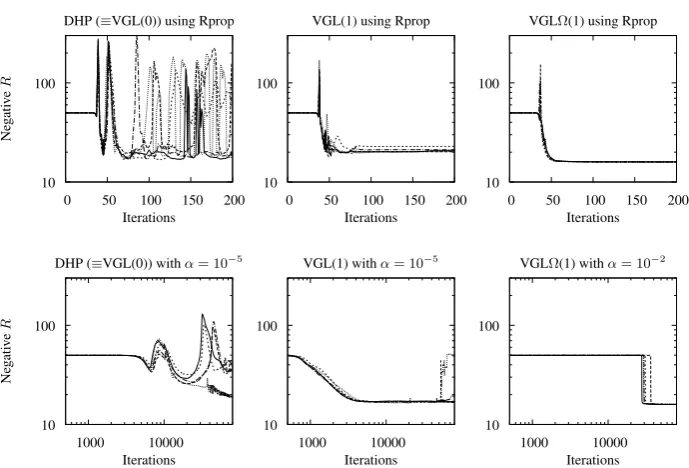
Figure 7.2 shows learning performance of the three algorithms, both with and
without RPROP. These graphs show the clear stability and performance advantages
of usingλ= 1and the chosenΩtmatrix.
The VGLΩ(1) algorithm shows near-to-monotonic progress in the later stages of
10 100
0 50 100 150 200
Ne
g
ati
v
e
R
Iterations DHP (≡VGL(0)) using Rprop
10 100
0 50 100 150 200 Iterations
VGL(1) using Rprop
10 100
0 50 100 150 200
Iterations VGLΩ(1) using Rprop
10 100
1000 10000
Ne
g
ati
v
e
R
Iterations DHP (≡VGL(0)) withα= 10−5
10 100
1000 10000 Iterations VGL(1) withα= 10−5
10 100
[image:23.595.98.443.87.321.2]1000 10000 Iterations VGLΩ(1) withα= 10−2
Figure 7.2 Results show learning progress for 5 typical random weight initialisations, for the problem of trying to learn 10 different trajectories. Results show increasing effectiveness (particularly in reduced volatility) for the three learning algorithms being considered, in the order that the graphs appear from left to right. The top row of graphs are all using RPROP to accelerate learning. The bottom row of graphs all use a fixed step-size parameterα.
present because RPROP causes the weight vector to traverse a significant
disconti-nuity in the value function that exists ath= 0,v= 0.
VGL(0) shows very far-from-monotonic behaviour in this problem.
7.5 CONCLUSIONS
We have defined the VGL(λ) algorithm, and proven its equivalence under certain
conditions to BPTT. VGL(1) with an Ωt matrix defined by 7.13 is thus a critic
learning algorithm that is proven to converge, under conditions stated in section
7.3.3, for a greedy policy and general smooth approximated critic. Although the
CONCLUSIONS 23
for research in that direction, particularly with the publication of Lemma 4. This
convergence proof has also given us insights into how theΩtmatrix can be chosen
and what its purpose is, at least for the case ofλ= 1with a greedy policy, and we speculate that similar choices could be valid forλ <1or non-greedy policies. In our experiment, we used a simplifiedΩtmatrix that was analytically derived and easy to
compute; but this may not always be possible, so an approximation to equation 7.13
may be necessary.
Our experiment has been a simple one with known analytical functions, but it has
demonstrated effectively the convergence properties of VGL(1) with the chosenΩt
matrix, and the relative ease with which it can be accelerated using RPROP. In this
experiment we found the convergence behaviour and optimality attained by VGL(1)
with the chosenΩtmatrix to be superior to VGL(1) withΩt=I, which in turn has
proved superior to VGL(0) (DHP) withΩt =I. The given experiment was quite
problematic for VGL(0) to learn and produce a stable solution, partly because in this
deceptively simple environment the major proportion of the total reward arrives in the
final time step, and partly because the lowcvalue chosen for equation 7.17 makes the
functionginto approximately a step-function, which implies that the surfaceR(~x, ~w) will be riddled with flat plateaus separated by steep cliffs.
It was surprising to the authors that the VGL(1) weight update has been proven to
be equivalent togradient ascent onRwhen previous research has always expected DHP (and therefore presumably its variant, VGL(1)) to begradient descent onE, whereEis the error functionE=P
t
G0t−Get
T Ωt
G0t−Get
REFERENCES
1. R. E. Bellman.Dynamic Programming. Princeton University Press, Princeton, NJ, USA, 1957.
2. C. M. Bishop.Neural Networks for Pattern Recognition. Oxford University Press, 1995. 3. K. Doya. Reinforcement learning in continuous time and space. Neural Computation,
12(1):219–245, 2000.
4. S. E. Fahlman. Faster-learning variations on back-propagation: An empirical study. In
Proceedings of the 1988 Connectionist Summer School, pages 38–51, San Mateo, CA, 1988. Morgan Kaufmann.
5. M. Fairbank. Reinforcement learning by value gradients.eprint arXiv:0803.3539, 2008. 6. M. Fairbank and E. Alonso. The divergence of reinforcement learning algorithms with
value-iteration and function approximation.eprint arXiv:1107.4606, 2011.
8. S. Ferrari and R. F. Stengel. Model-based adaptive critic designs. Handbook of learning and approximate dynamic programming, editors Jennie Si et al., pages 65–96, 2004. 9. D. Prokhorov and D. Wunsch. Adaptive critic designs. IEEE Transactions on Neural
Networks, September:997–1007, 1997.
10. M. Riedmiller and H. Braun. A direct adaptive method for faster backpropagation learning: The RPROP algorithm. InProc. of the IEEE Intl. Conf. on Neural Networks, pages 586– 591, San Francisco, CA, 1993.
11. R. S. Sutton. Learning to predict by the methods of temporal differences. Machine Learning, 3:9–44, 1988.
12. J. N. Tsitsiklis and B. Van Roy. An analysis of temporal-difference learning with function approximation. Technical Report LIDS-P-2322, 1996.
13. F.-Y. Wang, H. Zhang, and D. Liu. Adaptive dynamic programming: An introduction.
IEEE Computational Intelligence Magazine, pages 39–47, 2009.
14. C. J. C. H. Watkins.Learning from Delayed Rewards. PhD thesis, Cambridge University, 1989.
15. P. J. Werbos. Backpropagation through time: What it does and how to do it. InProceedings of the IEEE, volume 78, No. 10, pages 1550–1560, 1990.
16. P. J. Werbos. Approximating dynamic programming for real-time control and neural modeling. Handbook of Intelligent Control, editors White and Sofge, pages 493–525, 1992.
17. P. J. Werbos. Neural networks, system identification, and control in the chemical process industries. Handbook of Intelligent Control, editors White and Sofge, pages 283–356, 1992.