Trend following, risk parity and momentum in commodity futures

(1)

City, University of London Institutional Repository

Citation

:

Clare, A., Seaton, J., Smith, P. N. & Thomas, S. (2014). Trend following, risk parity and momentum in commodity futures. International Review of Financial Analysis, 31, pp. 1-12. doi: 10.1016/j.irfa.2013.10.001

This is the accepted version of the paper.

This version of the publication may differ from the final published

version.

Permanent repository link: http://openaccess.city.ac.uk/17846/

Link to published version

:

http://dx.doi.org/10.1016/j.irfa.2013.10.001

Copyright and reuse:

City Research Online aims to make research

outputs of City, University of London available to a wider audience.

Copyright and Moral Rights remain with the author(s) and/or copyright

holders. URLs from City Research Online may be freely distributed and

linked to.

City Research Online: http://openaccess.city.ac.uk/ publications@city.ac.uk

(2)

Electronic copy available at: http://ssrn.com/abstract=2126813

1

Trend Following, Risk Parity and Momentum in Commodity

Futures

Andrew Clare, James Seaton, Peter N. Smith† and Stephen Thomas*

*Cass Business School, London

†

University of York, UK

This Version: 11

th

_{December, 2012}

Abstract

We show that combining momentum and trend following strategies for individual commodity futures can lead to portfolios which offer attractive risk adjusted returns which are superior to simple momentum strategies; when we expose these returns to a wide array of sources of systematic risk we find that robust alpha survives. Experimenting with risk parity portfolio weightings has limited impact on our results though in particular is beneficial to long-short strategies; the marginal impact of applying trend following methods far outweighs momentum and risk parity adjustments in terms of risk-adjusted returns and limiting downside risk. Overall this leads to an attractive strategy for investing in commodity futures and emphasises the importance of trend following as an investment strategy in the commodity futures context.

(3)

2

1. Introduction

In this paper we contribute to the growing evidence that applying a trend following investment strategy to a variety of asset classes leads to enhanced risk adjusted returns. In particular we show that combining momentum and trend following strategies for individual commodity futures can lead to portfolios which offer attractive risk adjusted returns; when we expose these returns to a wide array of sources of systematic risk we find that robust alpha survives. Experimenting with risk parity portfolio weightings has limited impact on our results though is beneficial to long-short strategies; the marginal benefit of applying trend following methods far outweighs momentum and risk parity adjustments in terms of risk-adjusted returns and limiting downside risk.

Momentum strategies involve ranking assets based on their past return (often the previous twelve months) and then buying the winners and selling the losers. Momentum is one anomaly in the financial literature that has been demonstrated to offer enhanced future returns. Many studies since Jegadeesh and Titman (1993) have focussed on momentum at the individual stock level. More recently Asness et al (2012) find momentum effects within a wide variety of asset classes. In terms of commodity futures, Miffre and Rallis (2007) and Erb and Harvey (2006) were amongst the first to show that momentum strategies earn significant positive excess returns. The purpose of this paper is to show how a momentum strategy for commodity futures which also employs a trend following overlay can significantly enhance investment performance relative to both long only and long-short momentum strategies.

(4)

3

focused on equities with Wilcox and Crittenden (2005) and ap Gwilym et al (2010) as examples. Recent attempts at explaining the success of trend following include Faber (2007) who uses trend following as a means of tactical asset allocation and demonstrates that it is possible to form a portfolio that has equity-level returns with bond-level volatility. Ilmanen (2011) offers a variety of explanations as to why trend following may have been successful historically, including investor under-reaction to news and herding behaviour.

A few studies have sought to combine the momentum and trend-following strategies. Faber (2010) examines momentum and a form of trend following in equity sector investing in the United States. Antonacci (2012) analyses the returns from momentum trading of pairs of investments and then applies a quasi-trend following filter to ensure that the winners have exhibited positive returns. This is based on the argument that extreme past returns or volatility should be taken account of in identifying a risk factor to increase momentum profitability. The risk-adjusted performance of these approaches appears to be a significant improvement on benchmark buy-and-hold portfolios. Bandarchuk and Hilscher (2012) present a similar strategy arguing that many of the characteristics that have been identified as being correlated with, or explanations for, the presence of enhanced momentum profits are just related to extreme past returns. Conditioning on this effect, they find no role for characteristics such as book to market (Sagi and Seasholes, 2007), forecast dispersion (Verardo, 2009) and credit rating (Amramov et al, 2007) in raising momentum profitability. In this paper we direct attention to the ability of a trend following rule to enhance momentum profitability in commodity futures.

Behavioural and rational asset pricing explanations for momentum and trend following have been offered in the literature. Hong and Stein (1999) is representative of behavioural approaches which could generate momentum or trend following behaviour whilst Sagi and Seasholes (2007) examines trend behaviour in single risky assets which could be applicable to the construction of a momentum portfolio.

(5)

4

portfolios. Finally, in this paper we also examine how risk parity weighting affects strategy performance.

Section 2 contains a description of our data while in Section 3 we examine the role of momentum and trend following investment strategies along with different portfolio formation techniques using both risk parity and equal weighting portfolio construction methods;Section 4 presents the empirical results for applying these methods to our commodites’data while in Section 5 we control for both transactions’ costs and explore sources of systematic risk which may be present in our analysis.Section 6 concludes.

2. Data and Methods

The commodity futures data examined in this paper is the full set of DJ-UBS commodity excess return indices. These returns are inclusive of spot and roll gains but assume no returns on collateral put up1

The 28 commodities are:

. The full data period runs from January 1991 to June 2011. The period of study is 1992-2011 with all observations being monthly data. The first year of data is used to calculate trend-following signals and momentum rankings. Throughout the paper all values are total returns (unless specified) and are in US dollars.

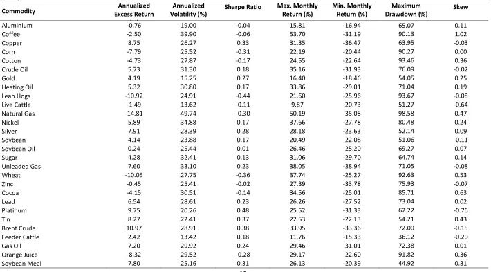
A summary of the properties of the returns series is shown in Table 1. The spread of variability and return is notable with some commodities such as natural gas and coffee showing a volatility of returns substantially higher than others, along with severe drawdowns and often negative risk-adjusted returns.The Sharpe ratios are generally unattractive as individual asset investments.There is also clear evidence of non-normality in returns.

(6)

5

3. Investment Strategies in Commodity Futures:Portfolio Weighting,Momentum and

Trend Following

We begin by reviewing two key aspects of portfolio formation for commodity futures, namely the justification for using trend following and/or momentum strategies in selecting individual assets together with the method of weighting those assets in the portfolio.

3.1 Momentum and Trend Following Strategies

A momentum strategy is a simple trading rule which involves taking a long investment position in rank-ordered, relatively good performing assets (winners) and a short position in those which perform relatively poorly (losers) over the same investment horizon. It is an explicit bet on the continuation of past relative performance into the future. Trend following, although closely related to momentum investing, is fundamentally different in that it does not order the past performance of the assets of interest, though it does rely on a continuation of, or persistence in, price behaviour based upon technical analysis. There is a tendency at times to use the terms ‘momentum’ and ‘trend following’ almost interchangeably, yet the former has a clear cross sectional element to it in that the formation of relative performance rankings is across the universe of stocks (or other securities) over a specific period of time, only to be continued in a time-series sense and eventually mean reverting after a successful ‘winning’ holding period. It should also be noted that momentum studies usually use monthly data whereas trend following rules are applied to all frequencies of data.

(7)

6

suggests that the typical Sharpe ratio for a single asset using a trend following strategy lies between 0 and 0.5 but rises to between 0.5 and 1 when looking at a portfolio.

3.2 Risk Parity vs Equal Portfolio Weights

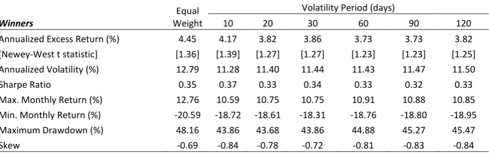
The first issue to deal with in forming portfolios of commodity futures is that of weights of individual assets. The vast differences in the volatility of returns to the commodities that we examine lead to the question of whether the portfolios formed based on a trend following or momentum strategy (or indeed any strategy, for that matter), are dominated by the volatility of the returns of individual commodities with the most extreme volatilities and drawdowns. In the data examined here, the commodities with the highest return volatility are Natural Gas, Coffee, Nickel, Unleaded Gas and Sugar, (see Table 1) In the simple equal-weighted 12-month momentum strategy portfolio evaluated below these commodities are over-represented when compared with equal average representation by 27% compared with the lowest volatility commodities Feeder Cattle, Live Cattle, Gold, Aluminium and Platinum. The resolution to this problem of reduced diversity of portfolio holdings that has developed in both markets and in the literature is risk-parity weighting2. This employs volatility weights rather than equal, market value or rule-of-thumb weights (such as the 60/40 equity/bond weights traditionally employed). The idea behind this is to weight assets inversely by their contribution to portfolio risk; this has the effect of overweighting low risk assets and in practice leads to massively overweight bond components of equity/bond portfolios in recent years (see Montier, 2010) and ensuing superior performance due to the bull market in bonds.

In this paper we employ realized volatility measures for constructing the volatility weights using a spread of windows of days over which volatility is computed. This type of measure has been shown by Andersen and Bollerslev (1998), amongst others, to provide an unbiased and efficient measure of underlying volatility3

2

See Dalio (2004) for an early justification for risk-parity weighting and Asness et al (2011) for a recent argument..

. Given the monthly frequency of the returns data, we compute realized volatility measures for between 10 and 120 days prior to

(8)

7

the date of the measurement of returns. The risk parity portfolios have the characteristic of increasing the relative diversity of portfolio holding of individual commodity futures. The 60-day risk-parity momentum portfolio shows an over-representation of high versus low volatility commodities across the whole dataset of only 2% when compared with equal average representation

The baseline portfolio returns against which we will evaluate all of the strategies in this paper are the equal weighted and risk parity long-only portfolios of all commodities whose characteristics are shown in Table 2. It can be seen that the average annual return in excess of the 3-month US Treasury Bill rate is 4.45% for the equally weighted portfolio. Average returns are somewhat lower for the basic risk parity portfolios, although both are significantly positive given the size of the Newey-West t-statistics employed throughout this paper. The trade-off of return against volatility is shown by the slightly lower volatility in risk parity portfolios. The Sharpe ratios for the equally weighted and risk parity portfolios are similar as indeed are the monthly maximum and minimum returns and maximum drawdown:there would seem to be little benefit in using risk parity as a portfolio construction technique for commodity futures.

Another metric for assessing the performance of the strategies examined in this paper is their returns in recent periods of market turbulence. This approach is proposed by Hurst, Johnson and Ooi (2010) in their assessment of risk parity portfolios. The periods we consider are the surprise increase in Fed interest rates(1994), the period of the Tech boom and separately bust(1999-2004), the period of easy credit and finally the credit crunch. Average returns of the baseline strategies are shown in Table 3 and show that the risk parity strategies have lower absolute average returns than the equally weighted strategy. The most pronounced differences between the two across the two most recent periods were when risk parity returns were somewhat lower during the period of easy credit and were a full 40 basis points more during the credit crunch. Below we monitor these measures along with more standard summary statistics.

4. Results

(9)

8

We consider a trend following rule that is popular with investors which is based on simple monthly moving averages of returns4. The buy signal occurs when the individual commodity future return moves above the average where we consider moving averages ranging from 6 to 12 months. The intuition behind the simple trend following approach is that while current market price is most certainly the most relevant data point, it is less certain whether the most appropriate comparison is a month or a year ago, (Ilmanen, 2011). Taking a moving average therefore dilutes the significance of any particular observation. With each of the rules, if the rule ‘says’ invest we earn the return on the commodity future over the relevant holding period which we fix at one month; however when the return ‘says’ do not invest we earn the return on cash over the holding period of one month. The rules are therefore binary: we either earn the return on the risky asset or the return on cash. In this case this return is the Treasury bill interest rate which has zero excess return. Previous research including Annaert, van Osslaer and Verstraete (2009) for equities, for example, suggests better performance from the longer moving averages examined in this paper.

Table 4 presents our results for both long positions in panel A and long-short positions in panel B. The long positions return either the one month excess return or zero depending on the trend following signal. The long-short strategies allow for short positions for those periods when the trend following buy signal is negative. All strategies show a positive excess return which is significantly higher than those for the passive positions shown in Table 2. Shorter length moving average signals provide a higher return than longer with the highest return for the 7-month moving average signal. These average excess returns are all significantly larger than zero. They are not, however, statistically significantly different from one another. The long only strategies provide the highest Sharpe ratio reflecting the generally rising market over the sample period and at around 0.7 are comfortably in the range suggested by Ilmanen (2011) of 0.5-1.0. Note that the annualised volatility without trend following in Table 2 at 12.79% for the equally weighted portfolio is roughly 50% more than the trend following equivalent(at around 7.94% in Table 4):this elevated return with much lower volatility (often a half to a third of a buy and hold equivalent) is a typical finding for a range of asset classes and historical periods (see Faber, (2007) and ap Gwilym et al, (2010)).

4

(10)

9

Note also that the maximum drawdown for trend following portfolios is roughly one-third that of long only equal weighting or risk parity strategies: again this is a typical finding that may be particularly desirable to investors.In addition,long-short strategies do provide even higher average returns which are generally more positively skewed,though the Sharpe ratios are inferior to the long-only case(see Table 4).Further in the most recent period of market turbulence during the credit crisis, trend following provided average returns of 0.64% per annum for long only, compared to -1.43% with no trend following (Table 3)

4.2 The Returns from Momentum Investing in Commodity Futures

The results from following a simple momentum investing strategy are shown in Table 5. The strategy we examine is based on the momentum in commodity returns over a range of prior periods ranging from 6 to 12 months. Portfolios are constructed for quartiles of highest (winner) and lowest (loser) commodity futures based on their cumulative return over the range of prior months. Returns are then computed for the month of the construction of the portfolios. Given the number of commodity futures that we examine, there are 7 returns in each of the winner and loser portfolios. The panels of summary statistics shown in Table 5 are for long positions in the winner and loser portfolios and long winner – short loser portfolios.

(11)

10

overall. Part of the motivation for introducing a trend following element to a momentum strategy in commodity futures is to reduce the skewness in returns and the associated crash risk.

Novy-Marx (2012) has recently raised the question of the relative performance of momentum strategies based on different length periods of momentum. His results show limited returns from shorter length periods of up to 6 months compared with longer periods between 6 and 12 months. Table 6 shows a comparison of four momentum periods for our commodity futures data. These show, contrasting with Novy-Marx, that returns and Sharpe ratios are higher for 12 month momentum returns than for short or medium length periods. Unlike evidence in Novy-Marx (2012), there is some evidence from column 2 of Table 6 that averaging over 2-6 months provides for a higher average return and Sharpe ratio than for the average of 7-12 months. However, these are both dominated by the 12 month period. The discontinuity in performance raises questions about the applicability of popular behavioural and rational explanations of the effectiveness of momentum strategies.

4.3 Risk Parity Trend Following and Momentum Portfolios

(12)

11

impact on the results but does lead to some overall improvement,especially with regard to maximum drawdowns.

What if we overlay trend following on the simple returns and apply risk-parity weighting?The results are shown in Table 8, where 7- and 12-month moving average-based strategies are reported,and may be compared with the equally weighted version in Table 4 which has no trend following. These show, as with the results for momentum strategies, that the biggest impact of risk – parity weighting is on loser portfolios and, consequently, on long winner – short loser portfolios. Average returns and Sharpe ratios are significantly higher for long-short portfolios for longer volatility calculation periods with the trend following overlay. These should also be compared with the risk-parity portfolios in Table 2 which do not adjust for trend following, where drawdowns are at least 3 times as big and Sharpe ratios are only half the size of Table 8. These results show that risk-parity weighting can have rather limited effects relative to equal weighting but that more predictable and substantial effects come from applying trend following.

Inker (2010) has raised a number of concerns with risk parity weighting in the context of strategies in equity and bond markets. These are mostly concerned with the use of leverage to extend the weight given to bonds in portfolios which we do not consider here. The remaining concern raised by Inker is that the attractiveness of previously low volatility return assets such as bonds might be overstated as they are subject to significant skewness risk. In our commodity futures data we do not see any substantial skewness risk with lower volatility commodities and therefore do not anticipate the increased weight attached to these commodities in the risk parity portfolio increasing skewness risk at the portfolio level. Indeed the addition of the trend following component reduces skewness in returns as is noted above.

4.4 The Performance of Combined Trend Following and Momentum Portfolios

(13)

12

following and 12-month momentum risk-parity portfolios based on a 60-day volatility calculation. Considering winner portfolios, the average excess returns from these strategies exceed those from any of the winner strategies examined thus far. Compared with momentum-only returns in Table 5 with, say a 12 month momentum period, the 7 month moving average trend following return at 12.90% is over 1.85% higher with a standard error of 0.27%. As a result of the impact of the lower volatility of trend following strategies, these higher returns are achieved at lower levels of volatility than in the case of momentum-only strategies and so have a higher Sharpe ratio than any of the previous strategies. There is no evidence of any skewness in these returns and they are also subject to lower maximum drawdown than previous strategies. Loser portfolios provide a consistently small negative and more volatile set of returns which are also not skewed. Winner-loser portfolios thus provide the highest set of returns for all trend-following moving average calculation periods and generate the highest average excess return of 15.94% and a Sharpe ratio of 0.82.(Table 9)These results show that amongst all momentum strategies, the introduction of trend following leads to reduced variability and a positive impact on skewness. If the risk-parity results in Table 9 are compared with those from equally weighted portfolios with similar momentum and moving average parameters in Table 10, it can be seen that risk parity leads to slightly higher average returns at a lower level of volatility. This is consistent with the original promoters of risk-parity portfolios and the evaluations of broader asset classes such as Asness et al (2012), for example. Finally, examining the periods of market turbulence, the final column of Table 3 shows that both equally weighted and risk parity returns from the combined 6-month trend following and 12-month momentum strategy provide positive returns over all of these periods and, in particular, the most recent credit crisis period where the winner-loser strategy delivered in excess of 3% pa.

(14)

13

significant enhanced average returns from these strategies is compensation for exposure to important risk factors is our next concern.

5. Understanding the profitability of strategy returns

5.1 Risk adjusted returns

The properties of returns presented thus far refer to unconditional returns from trend following and momentum strategies. In this section we examine whether these excess returns are explained by widely employed risk factors. For clarity, we examine the returns from particular strategies. These are equally and volatility-weighted versions of trend following based on a 7-month moving average window, momentum based on a 12-month prior period and the combination of these two strategies(Tables 9 and 10). In particular we examine estimates of alphas after regressing the returns from the strategies on two sets of risk factors which have been shown to explain substantial and significant amounts of the variation of returns in other markets; the Fama-French four US equity market factors, MKT, SMB, HML and UMD and, secondly, a wider set of market factors: the excess return from the Goldman Sachs Commodity Market Index (GSCI), the MSCI world equity market index (MSCI), the Barclays Aggregate Bond Index (BARBOND) and four hedge fund factors of Fung and Hsieh (2001): the PTFS Bond (SBD), Currency (SFX), Short-term Interest Rate (SIR) and Stock Index (STK) lookback straddle returns5. These are risk factors identified by Asness at al. (2012) and Menkhoff et al. (2012) as significant in the context of a range of markets including commodity futures and therefore provide a suitable benchmark against which to judge the levels of returns for the various strategies shown above.

The results of these estimates are shown in Table 11 where Newey-West t-statistics are shown in square brackets. Looking across all of the strategy returns and risk factors, there is little evidence that exposure to these factors is able to account for the returns from the strategies. Comparison of the estimated alphas from the two risk adjustment regressions with the raw alpha shows that the alphas remain large and significantly larger than zero. Most of the coefficients on the risk factors are small and insignificantly different from zero. Amongst the regressions for the long-only strategies the coefficients on the US equity market excess

5

(15)

14

return and, perhaps unsurprisingly, the return to the Cahart momentum factor (UMD) are positive and individually significantly different to zero. The regressions for the Fama-French factors are jointly significant but explain no more than 8.4% of the variation in returns in any case. For the wider set of market factors, the Goldman Sachs Commodity Market Index (GSCI) return has a positive and significant effect as do, marginally, the short-term interest rate and stock market hedge fund lookback straddle factors. These positive effects imply that the trend following and momentum strategies we examine are providing a hedge against the risks that these factors represent. These models explain more of the variation in returns. More than one third of the variation in the momentum returns is explained by the wider market factors, even if the alpha remains high. Amongst the long-short strategies, the estimation results in Table 12 show a lower level of significant exposure to the two sets of risk factors and a reduced fit. In both cases the estimated alphas are reduced less by the risk adjustment than in the long-only cases. The Fama-French momentum factor UMD is significantly priced in all of the first set of regressions, whilst the fit is generally below 10%. In the wider market factor models, the commodity futures strategies provide a hedge against US equity market momentum risk. Long-short trend following strategies load onto the world equity market return at a marginally significant level but the hedge fund factors are all insignificant at usual levels of significance. The fit in terms of R2of these models is around 5%.

The analysis of risk explanations for the trend following and momentum returns that we have found therefore suggests that whilst risk factors can provide a statistically significant contribution and explain some of the variation in returns, there remains a significant alpha which is at least two-thirds of the level of the raw excess returns.

5.2 Transactions costs

(16)

15

markets.6 In our calculations, for the range of commodities, the fixed cost element amounts to between 6 and 0.5 basis points, whilst the one tick, bid-ask spread is between 5.2 and 0.7 basis points. Having applied these costs, the differences between gross returns and returns net of transactions costs for the selected strategy returns evaluated in Section 5.1 can be seen in Table 13. The differences in average returns are not large at no more than 0.5% and well within one standard error of the gross returns. The extent to which trading costs have reduced over time due to improvements in the efficiency of trading technologies would make the net returns we analyse underestimates of performance in more recent parts of the sample period. Assessment of time variation in returns should take this into account.

5.3 Time-variation in the returns to investment strategies

The analysis presented thus far focuses on average returns and performance in particular episodes. The stability over time of momentum and trend following returns is clearly of interest – especially to those with shorter investment horizons. In Figures 1A-E we present average excess returns to a number of strategies calculated over rolling windows of 36 months. All of these returns show significant time variation. This is more apparent in the behaviour of momentum returns (Figure 1B) where the highest returns can be seen in the 2008-9 period having been lowest in the 2004-6 period. Trend following returns show lower time variation and remain at an enhanced level from 2009 to the end of the sample (Figure 1A). It can be seen from the figures that the addition of trend following to the momentum strategies dominates the difference in returns (Figure 1D): it matters less whether the portfolios are equally or risk-weighted (compare Figures 1B and C and D and E). This is of importance for those investors with shorter investment horizons.7 As noted above, it can be expected that the performance of returns net of transactions costs for all strategies could be enhanced by improvements in trading technologies in the later part of the sample period.

6. Conclusion

6

We apply these averages as the index data examined in this paper does not include actual contracts.

7

(17)

16

(18)

17

7. References

Andersen, T.G. and Bollerslev, T., (1998). “Answering the sceptics: Yes, Standard Volatility Models do Provide Accurate Forecasts”, International Economic Review, 39, 4, 885-905. Annaert, J., Van Osselaer, S., Verstraete, B., (2009). "Performance Evaluation of Portfolio Insurance Using Stochastic Dominance Criteria", Journal of Banking and Finance, 33, 272-280.

Antonacci, G., (2012). "Risk Premia Harvesting Through Momentum", Portfolio Management Associates.

ap Gwilym O., Clare, A., Seaton, J., Thomas, S., (2010). "Price and Momentum as Robust Tactical Approaches to Global Equity Investing", Journal of Investing, 19, 80-92.

Asness, C., Frazzini, A., and Pedersen, L., (2011). "Leverage Aversion and Risk Parity", AQR Capital Management working paper.

Asness, C., Moskowitz, T., and Pedersen, L., (2012). "Value and Momentum Everywhere",

Journal of Finance, (forthcoming). .

Avramov, D., Chordia, T., Jostova, G. and Philipov, A. (2007). “Momentum and Credit Rating”, Journal of Finance, 62, 407-427.

Baltas, A. and Kosowski, R. (2011). “Trend-following and Momentum Strategies in Futures Markets”, Imperial College, London, mimeo.

Bandarchuk, P. and Hilscher, J. (2012). “Sources of Momentum Profits: Evidence on the Irrelevance of Characteristics”, Review of Finance, (forthcoming).

Dalio, (2004). “Engineering Targeted Returns and Risks”, Bridgewater Associates Working Paper.

Daniel, K. and Moskowitz, T., (2011). "Momentum Crashes", Columbia Business School Research Paper.

Daniel, K., Jagannathan R. and Kim, S., (2012). “Tail Risk in Momentum Strategy Returns”, NBER Working Paper 18169.

Dow-Jones (2012). DJ-UBS CI: The Dow Jones-UBS Commodity Index Handbook, Dow Jones Indexes, New York.

Duffie, D., (2010). “Asset Pricing Dynamics with Slow-Moving Capital”, Journal of

Finance, 65, 1237-1267.

Erb, C., and Harvey, C., (2006). "The Tactical and Strategic Value of Commodity Futures",

Financial Analysts Journal, 62, 69-97.

Faber, M., (2007). “A Quantitative Approach to Tactical Asset Allocation”, Journal of

Investing, 16, 69-79.

(19)

18

Fung, W. and Hsieh, D., (2001). “The Risk in Hedge Fund Strategies: Theory and Evidence from Trend Followers”, Review of Financial Studies, 14, 2, 313-341.

Hong, H. and Stein, J., (1999). “A Unified Theory of Underreaction, Momentum Trading and Overreation in Asset Markets”, Journal of Finance, 54, 2143-2184.

Inker, B., (2010). "The Hidden Risks of Risk Parity Portfolios", GMO White Paper.

Hurst, B., Johnson, Z. and Ooi, Y.H., (2010). “Understanding Risk Parity”, AQR Capital Management Working Paper.

Hurst, B., Ooi, Y.H., Pedersen L., (2010). "Understanding Managed Futures", AQR Capital Management Working Paper.

Ilmanen A., (2011). Expected Returns. John Wiley & Sons, United Kingdom.

Jegadeesh, N. and Titman, S. (1993). “Returns to Buying Winners and Selling Losers: Implications for Stock Market Efficiency”, Journal of Finance, vol. 48, 65-91.

Koulajian, N., and Czkwianianc, P., (2011). "Know Your Skew: Using Hedge Fund Return Volatility as a Predictor of Maximum Loss", Quest Partners LLC.

Locke, P. and Venkatesh, P. (1997). “Futures Market Transactions Costs”, Journal of Futures

Markets, 17, 229-245.

Menkhoff, L., Sarno, L., Schmeling, M. and Schrimpf, A., (2012). “Currency Momentum Strategies”, Journal of Financial Economics, (forthcoming).

Montier, J., (2010). "I Want to Break Free, or, Strategic Asset Allocation ≠ Static Asset Allocation", GMO White Paper.

Miffre, J., Rallis, G., (2007), "Momentum Strategies in Commodity Futures Markets",

Journal of Banking & Finance, 31, 1863-1886.

Novy-Marx, R. (2012). “Is Momentum Really Momentum?”, Journal of Financial

Economics, 103, 429-453.

Ostgaard, S. (2008). "On the Nature of Trend Following", Last Atlantis Capital Management. Park, C. and Irwin, S., (2007). “What Do We Know About the Profitability of Technical Analysis”, Journal of Economic Surveys, 21, 786-826.

Sagi, J. and Seasholes, M. (2007). “Firm-specific Attributes and the Cross-section of Mometum”, Journal of Financial Economics, 84, 389-434.

Szakmary, A., Shen, Q., and Sharma, S., (2010). "Trend-Following Trading Strategies in Commodity Futures: A Re-Examination", Journal of Banking and Finance, 34, 409-426. Verardo, M. (2009). “Heterogenous Beliefs and Momentum Profits”, Journal of Financial

and Quantitative Analysis, 44, 795-822.

(20)

[image:20.842.70.780.121.514.2]

19

Table 1: Summary Statistics

The data are DJ-UBS commodity excess return indices. These returns are inclusive of spot and roll gains but assume no returns on collateral put up. Data period: 1992-2011 with all observations being monthly data. All data are total returns and are in US dollars .A full description of the construction of the indices can be found in Dow-Jones (2012).

Commodity _{Excess Return}Annualized

(%)

Annualized

Volatility (%) Sharpe Ratio

Max. Monthly Return (%)

Min. Monthly Return (%)

Maximum

Drawdown (%) Skew

Aluminium -0.76 19.00 -0.04 15.81 -16.94 65.07 0.11 Coffee -2.50 39.90 -0.06 53.70 -31.19 90.13 1.02 Copper 8.75 26.27 0.33 31.35 -36.47 63.95 -0.03 Corn -7.79 25.52 -0.31 22.19 -20.44 90.27 0.00 Cotton -4.73 27.87 -0.17 24.55 -22.64 93.46 0.36 Crude Oil 5.73 31.30 0.18 35.16 -31.93 76.09 -0.02 Gold 4.19 15.25 0.27 16.40 -18.46 54.05 0.25 Heating Oil 5.32 30.80 0.17 33.86 -29.01 71.04 0.19 Lean Hogs -10.92 24.91 -0.44 21.60 -25.96 93.67 -0.08 Live Cattle -1.49 13.62 -0.11 9.87 -20.73 51.27 -0.64 Natural Gas -14.81 49.74 -0.30 50.19 -35.08 98.58 0.47 Nickel 5.89 34.88 0.17 37.66 -27.78 80.48 0.24 Silver 7.91 28.39 0.28 28.18 -23.63 52.14 0.09 Soybean 4.14 23.88 0.17 20.49 -22.08 51.06 -0.11 Soybean Oil 0.24 25.44 0.01 26.46 -25.20 69.27 0.07 Sugar 4.28 32.41 0.13 31.06 -29.70 64.74 0.14 Unleaded Gas 7.60 33.10 0.23 38.05 -38.94 71.05 -0.08 Wheat -10.05 27.75 -0.36 37.74 -25.27 92.63 0.53 Zinc -0.45 25.41 -0.02 27.39 -33.78 75.93 -0.07 Cocoa -4.15 30.51 -0.14 34.56 -25.01 85.71 0.63 Lead 6.54 28.61 0.23 26.26 -27.52 73.04 0.02 Platinum 9.75 20.26 0.48 25.52 -31.33 62.22 -0.76

Tin 8.27 22.41 0.37 22.53 -22.13 54.21 0.43

(21)

[image:21.595.78.559.139.290.2]

20

Table 2: Risk Parity Portfolios - Monthly Rebalancing

This table shows the annualised average returns in percentages from portfolios formed from the 28 commodity futures of the DJ-UBSCI for the period Jan 1992 - Jun 2011. The risk-parity portfolios are formed using inverse relative volatility weights where relative volatility is calculated using between 10 and 120 days of return data prior to the portfolio formation date.

Equal Weight

Volatility Period (days)

Winners 10 20 30 60 90 120

(22)

[image:22.842.57.780.73.199.2]

21

Table 3: Average Annualized Returns over Periods of Interest Equal

Weight `Volatility Periods (days)

TF&MOM

10 20 30 60 90 120 EW RP

Surprise Fed Rate Hike -0.36 -0.36 -0.31 -0.31 -0.33 -0.36 -0.41 0.32 1.32

Tech Bubble 1.27 0.84 0.77 0.80 0.83 0.88 0.89 2.18 2.06

Tech Bust 0.32 0.03 0.06 0.08 0.05 0.06 0.08 1.03 1.53

Easy Credit 2.07 2.12 2.05 2.04 2.01 2.02 2.04 1.57 0.32

Credit Crunch -1.43 -1.04 -1.08 -1.09 -1.20 -1.25 -1.24 1.01 3.27

(23)

[image:23.595.70.555.74.403.2]

22

Table 4: Trend Following Portfolios - Monthly Trading Jan 1992 - Jun 2011 Moving Average Period (months)

6 7 8 9 10 11 12

Long-Only

Annualized Excess Return (%) [Newey-West t Statistic]

5.77 [3.06]

6.04 [3.20]

5.86 [3.13]

5.29 [2.90]

5.16 [2.87]

5.16 [2.81]

5.40 [2.88] Annualized Volatility (%) 7.93 7.94 7.84 7.80 7.74 7.81 7.79 Sharpe Ratio 0.73 0.76 0.75 0.68 0.67 0.66 0.69 Max. Monthly Return (%) 9.92 9.92 9.37 9.37 9.14 9.80 9.80 Min. Monthly Return (%) -7.11 -7.06 -7.06 -7.06 -6.91 -6.91 -6.91 Maximum Drawdown (%) 14.24 12.43 13.57 15.20 15.99 16.73 16.76

Skew 0.34 0.46 0.29 0.27 0.25 0.29 0.31

Long-Short

6.35 [2.66]

6.87 [2.84]

6.52 [2.77]

5.38 [2.38]

5.09 [2.27]

5.11 [2.39]

5.60 [2.63] Annualized Volatility (%) 10.19 10.29 10.04 10.03 10.12 10.07 10.00 Sharpe Ratio 0.62 0.67 0.65 0.54 0.50 0.51 0.56 Max. Monthly Return (%) 20.59 20.59 20.59 20.59 20.59 20.59 20.59 Min. Monthly Return (%) -9.25 -9.25 -9.25 -9.25 -9.46 -10.33 -10.33 Maximum Drawdown (%) 17.35 17.46 16.24 18.80 20.97 18.84 17.98

(24)

[image:24.595.70.556.83.542.2]

23

Table 5: Momentum Portfolios - Monthly Trading Jan 1992 - Jun 2011

Momentum Calculation Period (months)

6 7 8 9 10 11 12

Winners

9.95 [2.09] 8.52 [1.92] 5.91 [1.50] 4.93 [1.34] 7.10 [1.77] 10.67 [2.45] 11.12 [2.53] Annualized Volatility (%) 20.10 19.93 19.87 19.38 19.45 19.25 19.36 Sharpe Ratio 0.50 0.43 0.30 0.25 0.37 0.55 0.57 Max. Monthly Return (%) 17.75 16.61 16.61 16.81 17.47 16.81 16.81 Min. Monthly Return (%) -25.04 -27.72 -29.45 -26.52 -25.88 -25.88 -28.92 Maximum Drawdown (%) 48.67 50.70 50.63 54.11 52.73 49.80 51.56 Skew -0.14 -0.29 -0.44 -0.32 -0.26 -0.31 -0.56

Losers

0.16 [0.39] 1.13 [0.61] 1.65 [0.73] 0.58 [0.49] -0.83 [0.17] -2.49 [0.26] -1.16 [0.08] Annualized Volatility (%) 17.87 17.54 17.18 17.91 17.88 17.12 17.42 Sharpe Ratio 0.01 0.06 0.10 0.03 -0.05 -0.15 -0.07 Max. Monthly Return (%) 20.05 22.40 22.42 26.60 28.22 23.56 23.56 Min. Monthly Return (%) -19.83 -22.75 -21.78 -21.78 -20.64 -21.78 -21.14 Maximum Drawdown (%) 62.29 58.57 54.24 50.98 57.35 69.55 60.68 Skew 0.21 0.42 0.47 0.79 1.03 0.61 0.62

Long Winners-Short Losers

(25)

[image:25.595.69.431.91.540.2]

24

Table 6: 12-Month Momentum Subdivision - Monthly Trading Jan 1992 - Jun 2011

Momentum Calculation Period (months)

1 2-6 7-12 12 Winners

Annualized Excess Return (%) 8.08 9.24 7.57 11.12 Annualized Volatility (%) 18.53 19.53 18.29 19.36 Sharpe Ratio 0.44 0.47 0.41 0.57 Max. Monthly Return (%) 16.37 16.61 18.20 16.81 Min. Monthly Return (%) -17.92 -24.55 -26.32 -28.92 Maximum Drawdown (%) 48.88 49.58 63.56 51.56

Skew -0.13 -0.28 -0.47 -0.56

Losers

Annualized Excess Return (%) 0.93 1.62 -3.62 -1.16 Annualized Volatility (%) 18.00 17.80 16.90 17.42 Sharpe Ratio 0.05 0.09 -0.21 -0.07 Max. Monthly Return (%) 16.26 22.39 18.28 23.56 Min. Monthly Return (%) -17.31 -21.43 -16.31 -21.14 Maximum Drawdown (%) 66.47 62.15 71.33 60.68

Skew 0.07 0.36 0.32 0.62

Long Winners-Short Losers

Annualized Excess Return (%) 4.50 5.40 9.71 10.31 Annualized Volatility (%) 22.55 21.64 19.91 21.53 Sharpe Ratio 0.20 0.25 0.49 0.48 Max. Monthly Return (%) 17.23 23.60 15.36 19.89 Min. Monthly Return (%) -22.08 -22.39 -20.26 -26.66 Maximum Drawdown (%) 76.68 38.48 47.73 38.76

(26)

[image:26.595.69.510.84.551.2]

25

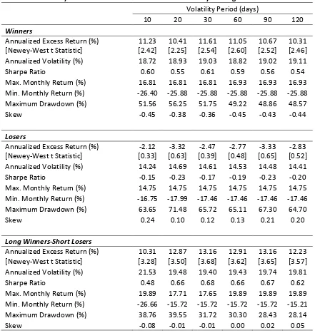
Table 7: Risk Parity 12-Month Momentum Portfolios - Monthly Trading Jan 1992 - Jun 2011 Volatility Period (days)

10 20 30 60 90 120

Winners

11.23 [2.42] 10.41 [2.25] 11.61 [2.54] 11.05 [2.60] 10.67 [2.52] 10.31 [2.46] Annualized Volatility (%) 18.72 18.93 19.03 18.82 19.02 19.11 Sharpe Ratio 0.60 0.55 0.61 0.59 0.56 0.54 Max. Monthly Return (%) 16.81 16.81 16.81 16.93 16.93 16.93 Min. Monthly Return (%) -26.40 -25.88 -25.88 -25.88 -25.88 -25.88 Maximum Drawdown (%) 51.56 56.25 51.75 49.22 48.86 48.57 Skew -0.45 -0.38 -0.36 -0.45 -0.43 -0.44 Losers

-2.12 [0.33] -3.32 [0.63] -2.47 [0.39] -2.77 [0.48] -3.33 [0.65] -2.83 [0.52] Annualized Volatility (%) 14.24 14.69 14.61 14.53 14.48 14.41 Sharpe Ratio -0.15 -0.23 -0.17 -0.19 -0.23 -0.20 Max. Monthly Return (%) 14.75 14.75 14.75 14.75 14.75 14.75 Min. Monthly Return (%) -16.75 -17.99 -17.46 -17.46 -17.46 -17.46 Maximum Drawdown (%) 63.65 71.48 65.72 65.11 67.30 64.70

Skew 0.24 0.10 0.12 0.13 0.21 0.20

Long Winners-Short Losers Annualized Excess Return (%) [Newey-West t Statistic]

10.31 [3.28] 12.87 [3.50] 13.16 [3.68] 12.91 [3.62] 13.16 [3.65] 12.23 [3.57] Annualized Volatility (%) 21.53 19.48 19.40 19.43 19.74 19.81 Sharpe Ratio 0.48 0.66 0.68 0.66 0.67 0.62 Max. Monthly Return (%) 19.89 17.71 17.65 19.89 19.89 19.89 Min. Monthly Return (%) -26.66 -15.72 -15.72 -15.72 -15.72 -15.21 Maximum Drawdown (%) 38.76 39.55 31.72 30.30 28.43 28.14

(27)

[image:27.595.70.556.86.708.2]

Table 8: Risk Parity Trend Following Portfolios - Monthly Trading Jan 1992 - Jun 2011

Volatility Period (days)

7-Month Moving Average Signal 10 20 30 60 90 120 180

Long-Only

5.01 [2.97] 5.10 [2.94] 5.22 [2.95] 5.35 [3.03] 5.40 [3.03] 5.51 [3.07] 5.51 [3.05] Annualized Volatility (%) 7.08 7.16 7.17 7.13 7.20 7.22 7.24 Sharpe Ratio 0.71 0.71 0.73 0.75 0.75 0.76 0.76 Max. Monthly Return (%) 8.62 9.25 9.41 9.73 9.62 9.67 9.76 Min. Monthly Return (%) -7.30 -6.98 -6.79 -6.73 -6.72 -6.74 -6.75 Maximum Drawdown (%) 13.30 13.06 12.78 12.65 12.69 12.74 12.77 Skew 0.12 0.22 0.33 0.37 0.33 0.35 0.36

Long-Short

12-Month Moving Average Signal

Long-Only

Long-Short

(28)

[image:28.595.72.555.91.587.2]

27

Table 9: Trend Following 60-Day Risk Parity 12-Month Momentum Portfolios - Monthly Jan 1992 - Jun 2011

Moving Average Period (months)

6 7 8 9 10 11 12

Winners

12.77 [3.39] 12.90 [3.49] 12.87 [3.41] 12.37 [3.30] 12.09 [3.26] 11.79 [3.10] 12.43 [3.23] Annualized Volatility (%) 16.17 16.41 16.54 16.64 16.56 16.83 16.91 Sharpe Ratio 0.79 0.79 0.78 0.74 0.73 0.70 0.73 Max. Monthly Return (%) 16.93 16.93 16.93 16.93 16.93 16.93 16.93 Min. Monthly Return (%) -13.00 -13.00 -13.00 -13.00 -13.00 -14.26 -14.26 Maximum Drawdown (%) 31.43 30.73 30.19 28.95 28.22 32.18 31.79

Skew 0.06 0.14 0.12 0.10 0.07 0.00 0.01

Losers

-3.07 [0.72] -4.02 [1.04] -3.46 [0.80] -3.26 [0.71] -3.07 [0.64] -3.23 [0.69] -3.40 [0.74] Annualized Volatility (%) 12.93 12.97 13.22 13.50 13.62 13.65 13.78 Sharpe Ratio -0.24 -0.31 -0.26 -0.24 -0.23 -0.24 -0.25 Max. Monthly Return (%) 14.75 14.75 14.75 14.75 14.75 14.75 14.75 Min. Monthly Return (%) -17.46 -17.46 -17.46 -17.46 -17.46 -17.46 -17.46 Maximum Drawdown (%) 62.18 66.65 66.46 66.79 64.66 64.64 66.52

Skew 0.04 0.07 0.07 0.07 0.05 0.05 0.08

(29)

[image:29.595.73.557.92.562.2]

28

Table 10: Equally Weighted Trend Following 12-Month Momentum Portfolios - Monthly Trading Jan 1992 - Jun 2011

Moving Average Period (months)

6 7 8 9 10 11 12

Winners

12.82 [3.31] 12.86 [3.42] 12.98 [3.36] 12.48 [3.27] 12.07 [3.18] 12.29 [3.16] 12.69 [3.24] Annualized Volatility (%) 16.47 16.54 16.69 16.77 16.90 17.23 17.29 Sharpe Ratio 0.78 0.78 0.78 0.74 0.71 0.71 0.73 Max. Monthly Return (%) 16.81 16.81 16.81 16.81 16.81 16.81 16.81 Min. Monthly Return (%) -14.11 -14.11 -14.11 -14.11 -14.11 -14.16 -14.16 Maximum Drawdown (%) 33.55 32.69 32.77 30.21 30.04 31.64 31.25

Skew 0.19 0.24 0.19 0.15 0.11 0.11 0.11

Losers

-1.91 [0.20] -2.95 [0.48] -1.82 [0.14] -1.75 [0.11] -1.30 [0.01] -1.60 [0.07] -1.91 [0.14] Annualized Volatility (%) 15.58 15.74 16.26 16.44 16.51 16.54 16.66 Sharpe Ratio -0.12 -0.19 -0.11 -0.11 -0.08 -0.10 -0.11 Max. Monthly Return (%) 23.56 23.56 23.56 23.56 23.56 23.56 23.56 Min. Monthly Return (%) -21.14 -21.14 -21.14 -21.14 -21.14 -21.14 -21.14 Maximum Drawdown (%) 56.91 63.28 60.35 61.98 57.66 59.31 62.94

Skew 0.50 0.57 0.81 0.77 0.74 0.74 0.74

(30)

[image:30.842.70.671.80.431.2]

29

Table 11: Risk Adjustment of Returns: Long Only Portfolios

Simple Average - Long Only

Average Average TF & MOM RP 1.126 TF RP 0.463

[3.49] [3.03] TF & MOM EW 1.125 MOMRP 1.026 [3.42] [2.60]

Equity Factors - Long Only

Alpha MKT SMB HML UMD R2 TF & MOM RP 0.877 0.233 -0.0036 0.0823 0.158 0.0844

[2.80] [3.24] [0.04] [0.92] [3.01]

TF & MOM EW 0.873 0.218 -0.0018 0.0877 0.173 0.0797 [2.83] [3.05] [0.02] [0.99] [3.19]

TF RP 0.35 0.104 0.00732 0.0546 0.0562 0.0420 [2.41] [2.61] [0.19] [1.44] [2.01]

MOM VW 0.649 0.436 0.0075 0.136 0.146 0.0705 [1.64] [3.54] [0.08] [1.47] [2.42]

Wider Market Factors - Long Only

Alpha GSCI MSCI BARBOND SBD SFX SIR STK R2 TF & MOM RP 0.913 0.0384 0.00581 -0.014 -2.026 0.603 1.711 2.211 0.183

[2.93] [6.09] [1.04] [0.75] [1.28] [0.50] [1.83] [1.04]

TF & MOM EW 0.94 0.0411 0.00213 -0.0166 -1.481 0.276 1.413 2.156 0.181 [3.22] [6.31] [0.39] [0.84] [0.98] [0.24] [1.74] [1.02]

TF RP 0.395 0.0158 0.00345 -0.0176 -0.602 0.549 -0.0533 1.171 0.192 [2.92] [5.61] [1.17] [2.28] [0.81] [1.00] [0.01] [1.55]

MOM RP 0.659 0.0444 0.0167 0.0134 -0.911 -0.245 -0.539 0.0656 0.356 [2.11] [6.96] [3.09] [0.44] [0.39] [0.18] [0.40] [0.02]

(31)

[image:31.842.69.682.85.411.2]

30

Table 12: Risk Adjustment: Long-Short Portfolios

Simple Average - Long-Short

Average Average TF & MOM RP 1.398 TF RP 0.565

[4.07] [2.92] TF & MOM EW 1.272 MOMRP 1.172 [3.41] [3.62]

Equity Factors - Long-Short

Alpha MKT SMB HML UMD R2 TF & MOM RP 1.238 -0.0064 -0.0014 0.042 0.263 0.0780

[3.46] [0.06] [0.02] [0.36] [3.75]

TF & MOM EW 1.11 -0.0948 0.0512 0.0998 0.296 0.116 [2.90] [0.85] [0.52] [0.70] [4.20]

TF RP 0.601 -0.122 -0.0307 -0.0299 0.0847 0.0644 [2.65] [1.25] [1.04] [0.46] [3.05]

MOM RP 0.93 0.142 0.0312 0.0866 0.225 0.0576 [2.85] [1.71] [0.37] [0.77] [3.05]

Wider Market Factors - Long-Short

Alpha GSCI MSCI BARBOND SBD SFX SIR STK R2 TF & MOM RP 1.37 0.0206 -0.0102 -0.016 -1.036 0.981 1.791 2.433 0.0497

[3.08] [2.28] [1.27] [0.55] [0.50] [0.48] [1.09] [0.77]

TF & MOM EW 1.42 0.0138 -0.0156 -0.0279 -2.437 0.368 1.838 3.799 0.0538 [3.22] [1.13] [1.80] [0.94] [1.09] [0.17] [1.23] [1.05]

TF RP 0.648 0.00241 -0.0091 -0.0276 -0.535 1.046 1.13 1.413 0.0415 [2.85] [0.54] [1.86] [1.95] [0.52] [0.94] [0.83] [1.14]

MOM RP 0.985 0.0215 -0.001 0.014 0.937 -0.294 0.129 -0.498 0.0482 [2.48] [2.39] [0.10] [0.43] [0.35] [0.16] [0.08] [0.14]

(32)

[image:32.842.79.580.97.182.2]

31 Table 13: Transactions Costs Adjustment

Average Returns - Long Only

Gross Net Gross Net Gross Net

TF & MOM RP 12.90 12.62 TF EW 6.04 5.91 TF RP 5.35 5.31 [3.49] [3.38] [3.20] [2.99] [3.03] [2.91] TF & MOM EW 12.86 12.52 MOM EW 11.12 10.83 MOM RP 11.05 10.76 [3.42] [3.37] [2.53] [2.48] [2.60] [2.54]

Average Returns - Long-Short

Gross Net Gross Net Gross Net

TF & MOM RP 15.94 15.65 TF EW 6.87 6.75 TF RP 6.41 6.37 [4.07] [3.99] [2.84] [2.79] [2.92] [2.86] TF & MOM EW 13.76 13.01 MOM EW 10.31 9.75 MOM RP 12.91 12.21 [3.41] [3.38] [2.82] [2.70] [3.62] [3.55]

(33)

Figure 1A

[image:33.595.72.399.116.568.2]

Rolling Average 36-month Returns for Five Commodity Strategies

Figure 1B

(34)

[image:34.595.73.400.70.278.2]

33 Figure 1D

[image:34.595.71.402.74.522.2]

(35)