Flexible Genetic Algorithm: A Simple and Generic
Approach to Node Placement Problems
IYu-Hui Zhanga,b, Yue-Jiao Gongb,∗, Tian-Long Guc, Yun Lid, Jun Zhangb,∗ aSchool of Data and Computer Science, Sun Yat-sen University, Guangzhou, China bSchool of Computer Science and Engineering, South China University of Technology,
Guangzhou, China
cGuilin University of Electronic Technology, Guilin, China dSchool of Engineering, University of Glasgow, Glasgow, U.K.
Abstract
Node placement problems, such as the deployment of radio-frequency identifica-tion systems or wireless sensor networks, are important problems encountered in various engineering fields. Although evolutionary algorithms have been success-fully applied to node placement problems, their fixed-length encoding scheme limits the scope to adjust the number of deployed nodes optimally. To solve this problem, we develop a flexible genetic algorithm in this paper. With variable-length encoding, subarea-swap crossover, and Gaussian mutation, the flexible genetic algorithm is able to adjust the number of nodes and their correspond-ing properties automatically. Offsprcorrespond-ing (candidate layouts) are created legibly through a simple crossover that swaps selected subareas of parental layouts and through a simple mutation that tunes the properties of nodes. The flexible genetic algorithm is generic and suitable for various kinds of node placemen-t problems. Two placemen-typical real-world node placemenplacemen-t problems, i.e., placemen-the wind farm layout optimization and radio-frequency identification network planning problems, are used to investigate the performance of the proposed algorithm. Experimental results show that the flexible genetic algorithm offers higher per-formance than existing tools for solving node placement problems.
Keywords: genetic algorithm (GA), node placement problem (NPP), RFID
network planning (RNP), variable-length encoding, wind farm layout optimization (WFLO)
IThis work was supported in part by the National Natural Science Foundation of China
(NSFC) Key Project under Grant 61332002, in part by the NSFC Youth Project under Grant 61502542, and in part by the NSFC Joint Fund with Guangdong Key Projects under Grant U1201258.
∗Corresponding author
1. Introduction
The node placement problem (NPP) is an important problem in many field-s, such as radio frequency identification (RFID) [1], wireless sensor networks (WSNs) [2], wind farm design [3], and oil and gas industry [4]. The task of an NPP solver is to place a number of nodes optimally in a given area to meet
5
certain predefined objectives. For this, there are mainly three issues to be ad-dressed: 1) the number of nodes being deployed; 2) the positions of the nodes; 3) their property settings.
NPPs have been studied separately in the literature. They have different names in different contexts. For example, in the field of WSNs, an NPP is
10
sometimes referred to as a ‘relay node placement problem’ [2, 5–8]. In other fields, specific terms such as RFID network planning (RNP) [1, 9–12], wind farm layout optimization (WFLO) [3, 13–16], and well placement optimization (WPO)[4, 17–19] problems are used. The definitions of the problems are dif-ferent, but have something in common. Noticing that a solver to one of the
15
problems may be applicable to the others with similar characteristics, this pa-per considers the problems in a generic prospective. To this end, we provide a general framework for NPPs and develop an approach capable of solving various NPP instances.
During the past decade, a substantial amount of research has been
under-20
taken to address ad hoc NPPs. One sort of approach is to use deterministic algorithms such as integer linear programming [20, 21], mixed integer program-ming [22, 23], geometric programprogram-ming [24], and some other approximation al-gorithms [6, 8, 25]. These alal-gorithms are designed for particular problems with precise models. The defect is that the strong assumptions made by the models
25
narrow the scope of application of the algorithms. On the other hand, an NPP is usually coupled with a series of constraints and has multiple objectives. These make the problem complex. As an example, the planning of RFID systems has been proven to be NP-Complete [26, 27].
Recently, the use of alternative methods such as heuristic [7], evolutionary
30
algorithms (EAs) [28, 29] and swarm intelligence (SI) [30] has attracted an increasing attention. In the literature, both EAs such as genetic algorithms (GAs) [31–36] and SI techniques such as particle swarm optimization (PSO) [10, 11, 37] have been utilized to tackle ad hoc NPPs. However, since an EA uses a fixed-length encoding scheme to represent a candidate solution, it is hard
35
to adjust the number of nodes.
To illustrate this, suppose a square area is given to place a number of nodes to meet predefined requirements. Fig. 1 shows the fixed-length encoding scheme used in [11, 31, 37–40], where n stands for the estimated number of nodes, and (xi, yi) andpi represent the coordinates and property setting of the i-th
40
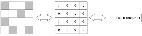
node respectively. However, it is difficult to accurately estimate the number of nodes in need, which plays a vital role in the assessment of layouts. Hence, the deployment in [11, 31, 37–40] still has room to improve. An alternative is a grid-based binary encoding approach as used in [10, 13, 15, 32–36], which divides the target area into multiple grids and uses a binary variable to indicate
45
x
1y
1p
1…
Node1 Node2 Noden
[image:3.612.168.443.190.260.2]x
2y
2p
2x
ny
np
nFigure 1: Fixed-length encoding scheme.
1 0 0 1
0 0 1 0
1 0 0 0
0 1 0 1
1001 0010 1000 0101
Figure 2: Grid-based method and its encoding scheme.
whether to place a node in the center of the corresponding grid, as shown in Fig. 2. In this way, a candidate solution (layout) can be represented by a binary string in a GA or PSO [41] to handle NPPs.
Although the grid-based approach is capable of pruning the number of n-odes, there are two disadvantages. First, because the positions of the nodes
50
are confined to the centers of the grids, the layout can only be optimized at a coarse-grained level. Second, it is inconvenient to incorporate additional prop-erties of nodes (such as the transmitted power of RFID readers [12]) into the optimization process.
To optimize the number of nodes as well as the deployment, a variable length
55
encoding scheme is required. In the literature, research efforts have been devot-ed to the design of variable length representations. One prominent research is the messy GA (mGA) proposed by Goldberget al. [42]. Suppose the solution to a problem consists of n-bits. The algorithm allows the chromosome length to be larger or less thann. When evaluating the fitness of an individual,
addi-60
tional processing is used to interpret the chromosome if its length is not exactly
n. A new operator called “cut and splice” is used to replace the traditional crossover operator. In [43], mGA is employed to solve the vehicle routing prob-lem. Kajitani et al. [44] proposed a variable length chromosome GA (VGA) for hardware evolution. The cut and splice operators are adopted in VGA to
65
realize recombination. In [45], Srikanthet al. proposed a variable-length GA for clustering. Each cluster is approximated by an ellipse and is encoded as a fixed length 0-1 bit string. The chromosome of an individual is allowed to grow or shrink through genetic operators, but the length of the chromosome must be a multiple of the length of a basic element (cluster). Hu and Yang [46] proposed a
70
simple path representation for GA to handle the path planning problem of mo-bile robots. The robot’s environment is given by a set of numbered grids and a path is encoded as a sequence of grid numbers. The first and last element of the sequence denotes the starting point and destination of the path. The number of intermediate nodes may vary from individual to individual. In [47], instead of
75
by a coordinate. Kim and Weck [48] proposed variable chromosome length GA (VCL-GA) to handle the structural topology optimization problem. The algo-rithm starts from a short chromosome and progressively lengthens the encoding to refine the individuals. Most of the encoding schemes are designed to handle a
80
specific kind of problem and cannot be generalized to tackle the node placement problem.
To overcome the shortcomings, this paper develops a flexible GA (fGA). The proposed fGA adopts a variable-length encoding for chromosomes eligibly to accommodate a variable number of nodes, with new crossover and mutation
85
operators designed accordingly. The encoding of fGA is based on the charac-teristics of nodes being deployed. Each element (gene) of the encoding has its specific meaning (the coordinates and properties of the nodes). The basic unit of the encoding is a single node and the building blocks of fGA are in the form of partial layouts instead of bit strings. The new crossover, termed subarea-swap
90
crossover, generates offspring by swapping selected subareas of one layout with another. The size and location of the crossover area are dynamically determined by the distribution of nodes. This ensures that the algorithm can be suited for node placement problems with different characteristics. Then, Gaussian mu-tation is performed on the offspring to adjust nodes positions and properties.
95
Compared to the existing methods, fGA has the following advantages:
1. Automatically adjusting the number of nodes in a legible and efficient manner.
2. Capable of optimizing the nodes’ positions and attached properties simul-taneously.
100
3. Enable a fine-grained placement of nodes (since the nodes’ positions are not restricted to the predetermined positions).
To investigate the performance of fGA, experiments on two real-world prob-lems (RNP and WFLO) are conducted. The experimental results show that fGA is superior to existing population-based optimization algorithms for NPPs.
105
The rest of this paper is organized as follows. The NPP is introduced in Section 2. Section 3 provides a detailed description of the proposed flexible genetic algorithm. Experiments on RNP and WFLO problems are presented in Section 4, with thorough analysis of the experimental results. The sensitivity of fGA to the parameter setting is also investigate in this section. Finally, Section
110
5 gives some concluding remarks and future research directions.
2. Problem Description
NPP is a common and important problem in many engineering fields. In this section, we give a formal description of the problem and provide a discussion on its components. Then, two typical real-world RNP and WFLO problems are
115
briefly described.
Node
+Position (x, y)
RFID Reader
+Transmitted Power
Wind Turbine
[image:5.612.221.392.126.224.2]+Hub Height +Rotor Diameter
…
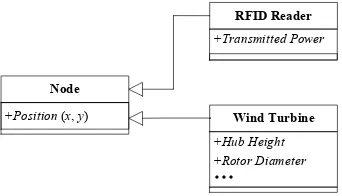
Figure 3: Structures of a Node: An RFID Reader and a Wind Turbine.
2.1. Formulation of the NPP
As its name suggests, the NPP consists of placing a number of nodes in a given area to meet specific requirements optimally. An instance of an NPP can be represented by a five-tuple (A, Node, S, F, Ω), where A is the area
120
for placement,Node is the structure of nodes (containing all the properties to be optimized), S is the set of candidate solutions, F is the set of objective functions, and Ω the set of constraints. A candidate solution that satisfies all the constraints is termed a feasible solution. The goal of an NPP solver is to find a feasible solution that yields the best objective values. In the following,
125
we briefly discuss the five components of an NPP.
1) Area for placement. The area for placement can be classified into two types.
The first contains a set of discrete points, and the nodes to be placed are re-stricted to these predetermined points. The second contains a continuous area, where the nodes can be positioned at any locations. Without loss of generality, this paper focuses on the second type. That is, the placement area is enclosed byNg geometric lines:
A={(x, y)|gi(x, y)≥0, i= 1,2, ..., Ng} (1)
2) Characteristics of nodes. A single node is the basic element of an NPP. There
are a number of nodes to be deployed. Each node hasNp properties:
Node ={pi|lbi≤pi≤ubi, i= 1,2, ..., Np} (2)
(p1,p2) is used to represent the position (x,y). lbi and ubi are the lower and upper bounds of the i-th property. The behavior of a node depends mostly on how these properties are set. Fig. 3 shows a class diagram of different kinds of nodes in the Unified Modeling Language, where the arrow denotes the
130
generalization (i.e., “is a”) relationship. The box on the left represents the basic structure of nodes and those on the right represent two specializations. The basic structure contains the most nontrivial property, namely, the position, while its specializations comprise other properties that also impact on the overall performance, such as the transmitted power of an RFID reader.
Besides, according to whether the properties of nodes are fixed or not, we can divide NPPs into two categories, i.e., homogeneous node placement problems (HoNPPs) and heterogeneous node placement problems (HeNPPs). Compared with an HoNPP, an HeNPP is more flexible, where the properties of each node can be set to any values within given ranges. Hence, the HeNPP is generally
140
more difficult to solve.
3) Candidate solution. A candidate solution comprises a number of nodes. It
can be denoted by a set of nodes whose positions are withinA:
X ={Nodei|(Nodei.p1,Nodei.p2)∈A, i= 1,2, ..., Nn} (3)
where Nn is the number of nodes in the solution. In the context of NPP, a candidate solution is also termed a layout. We use S to denote the set of all possible layouts.
4) Constraints. We use Ω to denote the set of constraints.
Ω ={Ci|Ci:Nodemi → {T, F}, i= 1,2, ..., Nc} (4)
where Nc is the number of constraints. Ci is an indicator function that maps
mi-fold Cartesian product of Node onto Boolean values. The return value T means that the corresponding constraint is satisfied. A candidate solutionX is feasible if:
∀i∈[1, Nc],∀Node1, ...,Nodemi ∈X :Ci(Node1, ...,Nodemi) =T (5)
Most constraints in NPPs impose restriction on the distances between the
de-145
ployed nodes. For example, WFLO requires that the distances between every two turbines be larger than a certain threshold to avoid damage of the wind turbine blades.
5) Objectives. F is a set of functions that project a layout to a single real value.
F ={fi|fi:S→R, i= 1,2, ..., No} (6)
No is the number of objectives. The objectives of NPPs vary from problem to problem. Some commonly seen objectives are briefly discussed as follows:
150
• Coverage: Taking WSNs as an example, every node (sensor) has a sensing
range. The objective is to cover as many targets as possible with the given number of nodes.
• Number of nodes: In practice, the number of nodes for placements is
usually not predefined, and it may be difficult to estimate the number of
155
nodes manually. On the premise that other objectives are not disturbed, the fewer nodes, the better the layout is. For some real-world applications where the cost of a node is relatively high, the number of nodes is a critical part in the assessment of a layout.
• Interference minimization: Ideally, all the nodes work cooperatively in
160
the area without disturbing one another. However, in a more realistic scenario, there is interference between the deployed nodes. For example, interference arises when several RFID readers interrogate a tag at the same time. This may cause misreading and lower the QoS of an RFID system. Hence, it is necessary to minimize interference when deploying
165
nodes.
• Other objectives: There are other objectives that worth mentioning, such
as the connectivity between deployed nodes, fault-tolerance and minimal energy consumption in communications.
2.2. Two Typical Real-World NPPs 170
In this subsection, we briefly discuss two instances of the NPP, i.e., the RNP and WFLO problems. More detailed descriptions of the two problems can be found in [12] and [3] respectively.
1) RFID Network Planning Problem. A typical RFID system is composed of
RFID tags, readers, and a host computer system. RFID tags are attached to
175
objects to be identified. RFID readers transmit interrogation signals and receive authentication replies from the tags. The host computer system processes and distributes relevant data. An RFID tag is said to be covered if both reader-to-tag and reader-to-tag-to-reader communications can be established. The RNP problem consists of placing a number of readers in the working area to cover as many tags
180
as possible while at the same time minimizing the number of deployed readers, interference, and the total transmitted power.
2) Wind Farm Layout Optimization Problem. The WFLO problem is
encoun-tered in the design of wind farms. The task is to determine the suitable number of wind turbines to be deployed and the positions of the turbines. If two turbines
185
are placed too close, the power generated by the downwind turbine will decrease significantly due to the existence of wake effects. Wake effects result from the changes in wind speed when wind turbines extract energy from the wind. The goal of an optimizer is to find the optimal deployment that maximizes the power produced and minimizes the cost of wind turbines.
190
3. Flexible Genetic Algorithm for NPPs
Evolutionary algorithms (EAs) are population-based optimization algorithm-s inalgorithm-spired by the mechanialgorithm-sm of biological evolution. Genetic algorithm (GA) ialgorithm-s among the most popular EAs. Owing to its global search ability and robustness, GAs have found widespread real-world applications [49–52]. In the literature,
195
genetic operators. In this section, we systematically introduce the algorithmic
200
components of fGA and then present the complete algorithm.
3.1. Genetic Representation
The fGA maintains a population containingpopsize individuals:
POP ={X1, X2, ..., Xpopsize} (7)
Each individualXi is a candidate solution (layout) containing a set of nodes:
Xi={Nodej|(Nodej.p1,Nodej.p2)∈A, j= 1,2, ..., ni} (8)
Nodej includes all properties to be optimized. ni is the number of nodes under assessment. We allow the individuals to have different number of nodes. There-fore, ni is not predefined. It is adjusted in the crossover operator during the
205
search process.
Procedure random initialization 01 for i from 1 to popsize 02 Xi←∅;
03 Generate a random number ni within [1, Nmax];
04 for j from 1 to ni
05 Create a new node Nodej;
06 for k from 1 to Np
07 Nodej .pk=lbk+(ubk-lbk)⋅rand(0,1);
08 end for 09 Xi←Xi∪{Nodej} ;
[image:8.612.203.410.317.436.2]10 end for 11 end for End Procedure
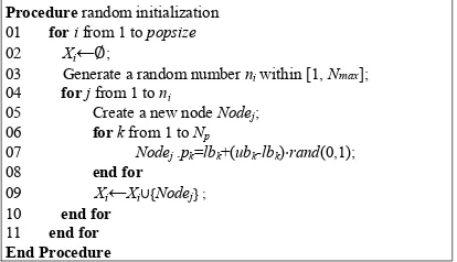
Figure 4: Pseudo code of random initialization.
3.2. Initialization
Assuming that no problem-specific knowledge is available, we use random initialization to generate the initial population. For each individualXi, a ran-dom number ni is generated within the range [1,Nmax], where Nmax is the
210
maximum number of nodes. Then, ni nodes are scattered over the working area. The initial positions of the nodes are randomly sampled from the area. Meanwhile, other properties (if any) are set to random values within their prede-termined feasible ranges. The pseudo code of the initialization process is given in Fig. 4.
215
3.3. Subarea-Swap Crossover
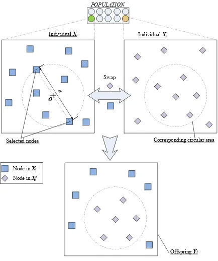
Since a variable-length encoding scheme is used, a location-based subarea-swap crossover independent of the number of nodes, is developed accordingly. Specifically, offspring are generated by swapping partial areas of two parental layouts. Fig. 5 illustrates the crossover operator. The detailed procedures are
220
as follows:
Step 1 For an individual Xi, generate a random number r within [0, 1]. If r
is smaller than the crossover probability Pc and Xi contains at least two nodes, go through the operations in Steps 2 and 3 to generate an offspringYi. Otherwise, the offspringYi is a copy ofXi.
225
Step 2 Select another individualXjat random from the population for crossover.
Step 3 Randomly select two nodes from Xi. Calculate the center O of these two nodes and their distanced. Then, draw a circle with centerO and radius d/2. Draw a corresponding circle with identical location and size in Xj. Swap the contents of the two subareas ofXi and Xj. The
230
resulting layout is retained as offspringYi.
The above procedure can be formulated as:
Yi=
(
XiNXj, randi< Pc
Xi, otherwise
(9)
whererandiis a random number uniformly distributed in [0, 1], and the operator
N
denotes operations in step 3. To facilitate a better understanding of the process, a pseudo code is provided in Fig. 6. It can be seen that the offspring
Yi may have different number of nodes from its parent Xi when the numbers
235
of nodes in the swapped subareas are different. The adaptive adjustment of the number of nodes relies largely on this crossover operator. Moreover, the subarea-swap crossover has introduced two dynamic features.
1) Locations of crossover areas. The locations of crossover areas are not
prede-fined, but determined by the positions of selected nodes. In this way, crossover
240
areas are automatically adjusted according to the distribution of nodes. No efforts will be wasted on inferior regions that are hardly visited by nodes, and a crossover area is very likely to locate in places where nodes are densely deployed.
2) Sizes of crossover areas. The size of a crossover area is also adaptively
ad-justed. It depends on the distance between two selected nodes. The diameter
245
of a circular crossover area ranges from dmin to dmax, where dmin denotes the distance of the pair of closest nodes and dmax the distance of the pair of farthest nodes. Therefore, the range is determined by the dispersion of the deployed nodes. Large crossover areas increase the population diversity while small crossover areas facilitate fine tuning.
250
3.4. Mutation
After the crossover operator, the offspring go through Gaussian mutation with probabilities Pm. In this process, the main task is to adjust the nodes properties. The mutation is performed on selected nodes of every individual to fine tune the nodes positions and other properties. Detailed descriptions of the
255
Node in Xi
Node in Xj
O
Selected nodes
POPULATION
Corresponding circular area
Offspring Yi
Individual Xi Individual Xj
[image:10.612.197.414.133.392.2]Swap
Figure 5: Illustration of crossover operation.
Procedure subarea-swap crossover 01 for each individual Xiin the population
02 randomly select another individual Xj ;
03 randomly select two nodes from Xi ;
04 calculate the center O of the two nodes; 05 calculate the distance d between the two nodes;
06 let crossover radius r = d/2;
07 offspring Yi←∅;
08 for each node Nodek in individual Xi
09 calculate the distance dk between Nodek and O;
10 if dk≥ r
11 Yi←Yi∪{Nodek};
12 end if
13 end for
14 for each node Nodek in individual Xj
15 calculate the distance dk between Nodek and O;
16 if dk < r
17 Yi←Yi∪{Nodek};
18 end if
19 end for
20 end for
End Procedure
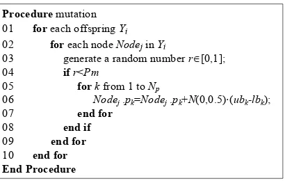
Procedure mutation 01 for each offspring Yi
02 for each node Nodej in Yi
03 generate a random number r[0,1];
04 if r<Pm
05 for k from 1 to Np
06 Nodej .pk=Nodej .pk+N(0,0.5)⋅(ubk-lbk);
07 end for
08 end if
09 end for
10 end for
End Procedure
Figure 6: Pseudo code of subarea-swap crossover.
For every node in Yi, generate a random real number r within [0, 1]. If
r < Pm, then perturbations are performed on the node’s properties by adding randomly scaled values. More specifically, for Nodej in Yi, the mutation is formulated as:
Nodej.pk=Nodej.pk+N(0,0.5)×(ubk−lbk), k= 1, ..., Np (10)
wherepk denotes the k-th property ofNodej. N(0, 0.5) is a Gaussian random number generator. Variablesubk and lbk represent the upper bound and lower bounds ofpk, respectively. Npis the total number of properties to be optimized. The utilization of Gaussian perturbation is inspired by evolutionary
pro-260
gramming (EP) [55], whose mutation is assisted by a Gaussian random number generator. This kind of mutation is very suitable for NPP for it enables the in-troduction of diversity adjustments, which greatly increases fGA’s local search ability. Note that 1) large perturbation factors cause relatively long jumps, 2) s-mall perturbation factors result in relatively slow progress. Hence, the standard
265
deviation of Gaussian distribution is empirically set to 0.5 to strike a balance. The pseudo code of the mutation operator is shown in Fig. 7.
Procedure subarea-swap crossover
01 for each individual Xi in the population 02 randomly select another individual Xj ; 03 randomly select two nodes from Xi ; 04 calculate the center O of the two nodes; 05 calculate the distance d between the two nodes; 06 let crossover radius r = d/2;
07 offspring Yi ←∅;
08 for each node Nodek in individual Xi
09 calculate the distance dk between Nodek and O;
10 if dk > r
11 Yi←Yi∪{Nodek};
12 end if
13 end for
14 for each node Nodek in individual Xj
15 calculate the distance dk between Nodek and O;
16 if dk < r
17 Yi←Yi∪{Nodek};
18 end if
19 end for
20 end for End Procedure
Procedure mutation 01 for each offspring Yi 02 for each node Nodej in Yi
03 generate a random number r[0,1];
04 if r<Pm
05 for k from 1 to Np
06 Nodej .pk=Nodej .pk+N(0,0.5)⋅(ubk-lbk);
07 end for
08 end if
[image:11.612.204.409.346.476.2]09 end for 10 end for End Procedure
Figure 7: Pseudo code of mutation.
3.5. Selection
Selection operator is followed right after the subarea-swap crossover and mutation. Each offspringYi originates from two parentsXi andXj. Since the
basic structure of Yi is inherited from Xi, Yi is considered as the immediate
successor of Xi. For clarity, we name Xi the primary parent of Yi. In the
selection process,Yicompetes withXifor admission to the next iteration. If the
offspring is better than its primary parent, then it survives for the next iteration. Otherwise, the primary parent continues its dominance and the offspringYi is
discarded. This procedure can be expressed as:
Xi=
(
Yi, ifYi is better thanXi
Xi, otherwise
No additional elitism strategies are required since the best individual will defi-nitely enter the next generation. The selection operator is strong at maintaining
270
the population diversity. Besides the operator described above, other selection operators (e.g., tournament selection and the roulette wheel selection) can also be used.
Crossover, mutation, and selection are repeated until the predefined termi-nation criterion is met. The overall procedure of fGA is summarized as follows:
275
Step 1 The population goes through the initialization process. In this process, each layout is generated by randomly deploying several nodes in the target area.
Step 2 For each individualXi in the population, generates an offspringYi by
performing the subarea-swap crossover on Xi and another randomly 280
selected individualXj.
Step 3 After the crossover operator, the offspring undergo mutation to search for better layouts through slight adjustments.
Step 4 The offspring are compared with their parents. If the offspring yield better objective values, they take the place of their parents. Otherwise,
285
they are discarded.
Step 5 Test if the termination criterion is met. If the answer is no, go to Step 2, otherwise, end the optimization process and output the best result ever found.
The parameters of fGA includepopsize,Pc, andPm. Compared to the
con-290
ventional GA, no additional parameters are introduced. Overall, fGA preserves the simple structure of GAs and only contains a few parameters.
4. Experimental Tests and Discussions
In this section, we apply the fGA to two real-world problems, i.e., the RN-P and WFLO problems. The RNRN-P and WFLO problems have the following
295
features:
1. The best number of nodes to be placed is hard to know. In RNP, the number of nodes is one of the objectives to be optimized, whereas in WFLO, the number of nodes has a direct influence on the fitness. On the other hand, RNP can be viewed as a small-scale problem since the
300
number of nodes (readers) to be included in a layout is relatively small. In comparison, WFLO is considered to be a mid- to large-scale problem. 2. Both problems take into account interference between nodes. In WFLO,
interference (wake effect) is a major concern for optimization to reduce power loss. Whereas in RNP, minimizing interference is one of the
objec-305
tives.
3. RNP falls in the category of HeNPP since the property (transmitted pow-er) of nodes (readers) is adjustable. In contrast, WFLO belongs to HoNPP because it employs the same type of nodes (wind turbines) with fixed prop-erties (hub height, rotor diameter, etc.).
310
4. The objectives of RNP and WFLO vary significantly. An RNP problem mainly aims at covering more tags, whereas a WFLO aims at capturing more wind energy.
The proposed algorithm is tested on both problems to make our experiments more comprehensive. In the next two subsections, experimental results on both
315
RNP and WFLO problems are presented, followed by a thorough analysis of the results. The algorithm developed in this paper (fGA) was written in C. All the following testing was done on a PC with Intel Core i3-3240 CPU.
4.1. Experiments on RNP
1) Test cases. Twelve test cases [12], namely C30, C50, C100, R30, R50, R100,
320
R30a, R50a, R100a, R30b, R50b, and R100b are used to examine the perfor-mance of fGA on RNP. They are based on a 50m×50m working area. Letter ‘C’ indicates that the tags in the working area are clustered distributed, where-as letter ‘R’ means uniform distribution of tags. The number behind a letter represents the number of tags included in the working area. It is clear that
325
instances labeled ‘R’ are harder than those labeled ‘C’, and more tags included in the working area, more complex the instance is. Therefore, R100, R100a, and R100b are the hardest among the twelve instances.
2) Fitness evaluation. RNP has four objectives, i.e., to maximize the tag
cov-erage, minimize the number of readers, minimize interference, and minimize the
330
sum of the total transmitted power. The objectives are listed in the order of precedence. It is considered that the coverage is the most important objective, followed by the other three one after another. It is an effective way to compare the individuals (solutions) in a hierarchical manner as in [12]. Specifically, when comparing two solutions, we first concentrate on their coverage rates. The one
335
with a higher coverage rate is judged to be better. If the two solutions have the same coverage rate, then the one uses fewer readers is better. The third and fourth objectives are compared accordingly.
3) Algorithms for comparison. The algorithms for comparison are grouped as
follows:
340
G1) GA-16 and GA-25: Two grid-based GAs with elitism strategy, which di-vide the working area into 4×4 grids and 5×5 grids respectively.
G2) GPSO, VNPSO, and SA-PSO: Three PSO algorithms using fixed-length encoding scheme. GPSO and VNPSO are with global and von Neumann topologies respectively. SA-PSO [56] is a recently proposed algorithm for
345
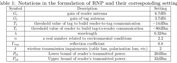
Table 1: Notations in the formulation of RNP and their corresponding settings
Symbol Description Setting
Gr gain of reader antenna 6.7dBi
Gt gain of tag antenna 3.7dBi
Tt threshold value of tag to build reader-to-tag communication −14dBm
Tr threshold value of reader to build tag-to-reader communication −80dBm
λ wavelength 0.328m
n a real number related to environmental conditions 2.2
Γtag reflection coefficient 0.8
δ wireless transmission impairments (cable loss, polarization loss, etc) 2 Plb Lower bound of reader’s transmitted power. 20dBm
Pub Upper bound of reader’s transmitted power. 33dBm
G3) GPSO-RNP and VNPSO-RNP [12]: Two state-of-the-art PSO algorithms with tentative reader elimination for solving RNP.
G4) GA-WMN [53]: A genetic algorithm originally designed for the wireless mesh network planning problem. It is adapted here to tackle the RNP
350
problem.
4) Parameter setting. The notations in the formulation of the RNP [12] and
their corresponding settings are summarized in Table 1. The parameters of the fGA are set as follows: popsize = 100; Pc = 0.9; Pm = 0.1. Parameters of GA-16 and GA-25 are set the same as the fGA. The parameters of GA-WMN
355
are set according to [53]. Since GPSO, VNPSO and SA-PSO use fixed-length encoding scheme (as shown in Fig. 1), the number of readers is fixed atNmax/2. The swarm size is set to 20. The inertia weight is initialized to 0.9 and linearly decreases to 0.4 with respect to iterations. The accelerating coefficients are set as
c1=c2 = 2.0. Parameters of GPSO-RNP and VNPSO-RNP are set according
360
to [12]. The maximum number of readers available for placement is 12, namely,
Nmax = 12. All algorithms terminate after 400,000 fitness evaluations. Each algorithm is run 50 times for each test case to obtain statistically reliable results.
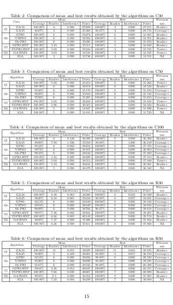
5) Experimental results and discussion. Experimental results on the twelve
cas-es are reported in Tablcas-es 2-13. The Wilcoxon rank-sum tcas-est (at the 0.05
signifi-365
cance level) is used to determine whether the results obtained by the four groups of algorithms are significantly different from those of the fGA. The statistical reports are listed in the last column of each table. ‘Coverage+’ indicates that the coverage rate obtained by fGA is significantly higher than the algorithm for comparison. By analogy, ‘Reader+’ means that the number of deployed readers
370
of fGA is significantly less than the other algorithm. ‘Power+’ is interpreted in the same way.
The first group of test cases (C30, C50, and C100) contains clustered dis-tributed tags, which is comparatively easy to solve. The experimental results on these cases are given in Tables 2-4. It can be seen that except for GA-25,
375
all the algorithms manage to reach 100% coverage rate at least once. GA-25 fails to reach 100% coverage rate in C30 and C100 in all 50 runs, and the three algorithms based on fixed-length encoding scheme (GPSO, VNPSO, and SA-PSO) fail occasionally in C50 and C100. In comparison, GA-16, GPSO-RNP,
Table 2: Comparison of mean and best results obtained by the algorithms on C30
Case Mean Best Wilcoxon test Coverage Readers Interference Power Coverage Readers Interference Power
G1 GA-16 100.00% 4 0.000 27.608 100.00% 4 0.000 27.011 Reader+ GA-25 86.67% 3 0.000 25.360 86.67% 3 0.000 24.774 Coverage+
G2
GPSO 100.00% 6 0.000 35.074 100.00% 6 0.000 31.865 Reader+ VNPSO 100.00% 6 0.000 34.762 100.00% 6 0.000 31.951 Reader+ SA-PSO 100.00% 6 0.000 35.096 100.00% 6 0.000 31.872 Reader+ G3 GPSO-RNP 100.00% 3.18 0.000 35.511 100.00% 3 0.000 33.948 Reader+ VNPSO-RNP 100.00% 3.04 0.000 35.034 100.00% 3 0.000 33.535 Power+ G4 GA-WMN 100.00% 3.03 0.000 34.550 100.00% 3 0.000 33.597 Power+ fGA 100.00% 3 0.000 33.736 100.00% 3 0.000 33.551 NA
Table 3: Comparison of mean and best results obtained by the algorithms on C50
Algorithm Mean Best Wilcoxon test Coverage Readers Interference Power Coverage Readers Interference Power G1 GA-16 100.00% 5.04 0.000 35.213 100.00% 5 0.000 35.266 Power+
GA-25 100.00% 6 0.000 34.874 100.00% 6 0.000 34.524 Reader+
G2
GPSO 95.60% 6 0.000 35.170 100.00% 6 0.000 31.852 Coverage+ VNPSO 99.20% 6 0.000 35.023 100.00% 6 0.000 31.742 Coverage+ SA-PSO 97.60% 6 0.000 35.305 100.00% 6 0.000 31.833 Coverage+
[image:15.612.136.476.140.230.2]G3 GPSO-RNP 100.00% 5.04 0.000 36.244 100.00% 5 0.000 33.418 Power+ VNPSO-RNP 100.00% 5.06 0.000 36.565 100.00% 5 0.000 34.522 Reader+ G4 GA-WMN 100.00% 5 0.000 31.927 100.00% 5 0.000 31.896 Power+ fGA 100.00% 5 0.000 31.816 100.00% 5 0.000 31.729 NA
Table 4: Comparison of mean and best results obtained by the algorithms on C100
Algorithm Mean Best Wilcoxon test Coverage Readers Interference Power Coverage Readers Interference Power G1 GA-16 100.00% 8 0.128 36.399 100.00% 8 0.099 36.304 Reader+
GA-25 99.00% 7.94 1.396 37.658 99.00% 7 1.290 36.159 Coverage+
G2
GPSO 98.34% 6 0.002 38.652 100.00% 6 0.000 37.374 Coverage+ VNPSO 99.72% 6 0.000 38.167 100.00% 6 0.000 36.803 Coverage+ SA-PSO 98.33% 6 0.000 38.632 100.00% 6 0.000 37.282 Coverage+
[image:15.612.139.477.253.337.2]G3 GPSO-RNP 100.00% 5.16 0.000 38.800 100.00% 5 0.000 37.513 Reader+ VNPSO-RNP 100.00% 5.04 0.000 38.513 100.00% 5 0.000 37.449 Power+ G4 GA-WMN 100.00% 5.33 0.000 36.641 100.00% 5 0.000 36.561 Reader+ fGA 100.00% 5 0.000 36.479 100.00% 5 0.000 36.342 NA
Table 5: Comparison of mean and best results obtained by the algorithms on R30
Algorithm Mean Best Wilcoxon test Coverage Readers Interference Power Coverage Readers Interference Power
G1 GA-16 100.00% 8.48 0.063 38.280 100.00% 8 0.103 38.592 Reader+ GA-25 90.00% 6.18 0.065 35.634 90.00% 6 0.057 34.941 Coverage+
G2
GPSO 92.13% 6 0.000 38.849 100.00% 6 0.000 38.842 Coverage+ VNPSO 94.53% 6 0.000 38.849 100.00% 6 0.000 38.656 Coverage+ SA-PSO 90.89% 6 0.000 38.766 96.67% 6 0.000 38.618 Coverage+ G3 GPSO-RNP 99.87% 7.46 0.002 39.821 100.00% 6 0.000 39.265 Reader+
VNPSO-RNP 100.00% 6.86 0.003 40.143 100.00% 6 0.000 39.574 Reader+ G4 GA-WMN 99.89% 7.37 0.000 37.306 100.00% 6 0.000 37.856 Reader+ fGA 100.00% 6.26 0.000 37.811 100.00% 6 0.000 37.860 NA
Table 6: Comparison of mean and best results obtained by the algorithms on R50
Algorithm Mean Best Wilcoxon test Coverage Readers Interference Power Coverage Readers Interference Power
G1 GA-16 100.00% 11 0.051 38.695 100.00% 11 0.043 38.835 Reader+ GA-25 94.00% 8 0.169 36.081 94.00% 8 0.057 36.743 Coverage+
G2
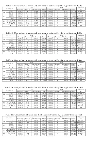
[image:15.612.137.477.359.538.2]Table 7: Comparison of mean and best results obtained by the algorithms on R100
Algorithm Mean Best Wilcoxon test Coverage Readers Interference Power Coverage Readers Interference Power
G1 GA-16 100.00% 11 0.819 39.395 100.00% 11 0.552 39.759 Reader+ GA-25 94.00% 9.14 0.676 38.349 94.00% 9 0.406 38.060 Coverage+
G2
GPSO 91.18% 6 0.001 40.074 95.00% 6 0.000 40.098 Coverage+ VNPSO 94.14% 6 0.001 40.333 97.00% 6 0.044 40.657 Coverage+ SA-PSO 91.33% 6 0.009 39.961 95.00% 6 0.000 40.782 Coverage+ G3 GPSO-RNP 99.74% 9.24 0.118 41.505 100.00% 8 0.000 40.925 Coverage+ VNPSO-RNP 100.00% 8.44 0.242 41.462 100.00% 8 0.000 41.031 Reader+ G4 GA-WMN 100.00% 8.97 0.011 39.686 100.00% 8 0.000 39.363 Reader+ fGA 100.00% 8 0.000 40.094 100.00% 8 0.000 39.660 NA
Table 8: Comparison of mean and best results obtained by the algorithms on R30a
Algorithm Mean Best Wilcoxon test Coverage Readers Interference Power Coverage Readers Interference Power G1 GA-16 100.00% 8.07 0.006 35.829 100.00% 8 0.000 35.755 Reader+
GA-25 86.67% 7.13 0.033 34.551 86.67% 7 0.000 32.260 Coverage+
G2
GPSO 93.44% 6 0.000 38.629 100.00% 6 0.000 38.653 Coverage+ VNPSO 98.11% 6 0.000 38.635 100.00% 6 0.000 37.632 Coverage+ SA-PSO 94.89% 6 0.003 38.950 100.00% 6 0.000 37.600 Coverage+
[image:16.612.136.476.139.227.2]G3 GPSO-RNP 100.00% 6.27 0.003 40.040 100.00% 5 0.000 39.861 Reader+ VNPSO-RNP 100.00% 6 0.001 40.139 100.00% 6 0.000 39.574 Reader+ G4 GA-WMN 99.89% 6.5 0.000 36.925 100.00% 6 0.000 36.291 Reader+ fGA 100.00% 5.4 0.000 37.967 100.00% 5 0.000 38.529 NA
Table 9: Comparison of mean and best results obtained by the algorithms on R50a
Algorithm Mean Best Wilcoxon test Coverage Readers Interference Power Coverage Readers Interference Power G1 GA-16 100.00% 8.1 0.145 36.983 100.00% 8 0.042 36.791 Reader+
GA-25 92.00% 8.6 0.215 37.047 92.00% 8 0.140 37.017 Coverage+
G2
GPSO 96.33% 6 0.000 39.669 100.00% 6 0.000 39.073 Coverage+ VNPSO 98.80% 6 0.000 39.586 100.00% 6 0.000 38.565 Coverage+ SA-PSO 95.53% 6 0.000 39.468 100.00% 6 0.000 39.210 Coverage+
[image:16.612.140.476.255.338.2]G3 GPSO-RNP 100.00% 7.17 0.007 40.993 100.00% 6 0.000 40.661 Power+ VNPSO-RNP 100.00% 7.037 0.009 41.155 100.00% 6 0.000 40.782 Power+ G4 GA-WMN 100.00% 7.37 0.000 38.193 100.00% 7 0.000 37.455 Reader+ fGA 100.00% 6.67 0.000 37.948 100.00% 6 0.000 37.912 NA
Table 10: Comparison of mean and best results obtained by the algorithms on R100a
Algorithm Mean Best Wilcoxon test Coverage Readers Interference Power Coverage Readers Interference Power
G1 GA-16 100.00% 10.17 1.191 39.004 100.00% 10 0.878 39.832 Reader+ GA-25 92.00% 9.77 0.811 38.273 92.00% 9 0.686 37.876 Coverage+
G2
GPSO 92.37% 6 0.012 40.116 97.00% 6 0.000 40.782 Coverage+ VNPSO 95.70% 6 0.014 40.480 97.00% 6 0.000 40.396 Coverage+ SA-PSO 92.50% 6 0.013 40.274 98.00% 6 0.000 40.782 Coverage+ G3 GPSO-RNP 96.67% 8.03 0.839 42.284 100.00% 8 0.000 41.489 Coverage+ VNPSO-RNP 96.67% 8.83 1.008 43.297 100.00% 8 0.000 41.850 Coverage+ G4 GA-WMN 100.00% 8.8 0.003 39.676 100.00% 8 0.000 39.456 Reader+
fGA 100.00% 8 0.000 39.920 100.00% 8 0.000 39.231 NA
Table 11: Comparison of mean and best results obtained by the algorithms on R30b
Algorithm Mean Best Wilcoxon test Coverage Readers Interference Power Coverage Readers Interference Power
G1 GA-16 100.00% 8.87 0.003 35.973 100.00% 8 0.000 34.696 Reader+ GA-25 93.33% 6.4 0.000 33.502 93.33% 6 0.000 33.343 Coverage+
G2
GPSO 96.89% 6 0.000 38.527 100.00% 6 0.000 37.984 Coverage+ VNPSO 99.33% 6 0.000 38.720 100.00% 6 0.000 37.849 Coverage+ SA-PSO 98.22% 6 0.000 38.817 100.00% 6 0.000 38.249 Coverage+ G3 GPSO-RNP 100.00% 5.97 0.000 40.036 100.00% 4 0.000 38.817 Reader+
VNPSO-RNP 100.00% 5.87 0.002 40.090 100.00% 4 0.000 38.875 Reader+ G4 GA-WMN 100.00% 6.1 0.000 36.958 100.00% 5 0.000 37.719 Reader+ fGA 100.00% 4.13 0.000 38.361 100.00% 4 0.000 38.276 NA
[image:16.612.137.475.366.460.2]Table 12: Comparison of mean and best results obtained by the algorithms on R50b
Algorithm Mean Best Wilcoxon test Coverage Readers Interference Power Coverage Readers Interference Power G1 GA-16 100.00% 10.27 0.110 38.363 100.00% 10 0.092 37.717 Reader+
GA-25 96.00% 8.67 0.405 37.960 96.00% 8 0.340 37.766 Coverage+
G2
GPSO 95.93% 6 0.003 39.835 100.00% 6 0.000 39.754 Coverage+ VNPSO 98.07% 6 0.000 39.825 100.00% 6 0.000 39.238 Coverage+ SA-PSO 95.53% 6 0.000 39.685 100.00% 6 0.000 39.634 Coverage+
G3 GPSO-RNP 100.00% 6.93 0.032 41.040 100.00% 6 0.000 39.901 Reader+ VNPSO-RNP 100.00% 6.97 0.034 41.066 100.00% 6 0.000 40.078 Reader+ G4 GA-WMN 100.00% 7.9 0.000 38.270 100.00% 7 0.000 38.435 Reader+ fGA 100.00% 6 0.000 38.942 100.00% 6 0.000 38.532 NA
Table 13: Comparison of mean and best results obtained by the algorithms on R100b
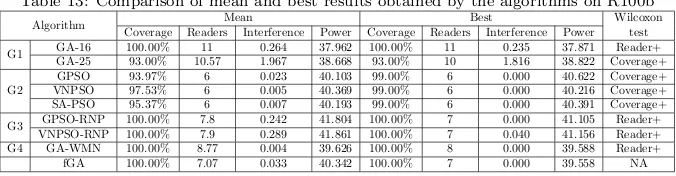
Algorithm Mean Best Wilcoxon test Coverage Readers Interference Power Coverage Readers Interference Power G1 GA-16 100.00% 11 0.264 37.962 100.00% 11 0.235 37.871 Reader+
GA-25 93.00% 10.57 1.967 38.668 93.00% 10 1.816 38.822 Coverage+
G2
GPSO 93.97% 6 0.023 40.103 99.00% 6 0.000 40.622 Coverage+ VNPSO 97.53% 6 0.005 40.369 99.00% 6 0.000 40.216 Coverage+ SA-PSO 95.37% 6 0.007 40.193 99.00% 6 0.000 40.391 Coverage+
G3 GPSO-RNP 100.00% 7.8 0.242 41.804 100.00% 7 0.000 41.105 Reader+ VNPSO-RNP 100.00% 7.9 0.289 41.861 100.00% 7 0.040 41.156 Reader+ G4 GA-WMN 100.00% 8.77 0.004 39.626 100.00% 8 0.000 39.588 Reader+ fGA 100.00% 7.07 0.033 40.342 100.00% 7 0.000 39.558 NA
VNPSO-RNP, GA-WMN, and fGA have shown their high stability in this group
380
of cases. As reported in Tables 2-4, they achieve the coverage goal in every run. The difference between the results obtained by VNPSO-RNP, GA-WMN, and fGA is moderate. Nevertheless, from the perspective of energy-saving, fGA suc-ceeds in consuming less transmitted power than VNPSO-RNP and GA-WMN. The second group of test cases (R30, R50, R100, R30a, R50a, R100a, R30b,
385
R50b, and R100b) is more difficult than the first group. The solutions found by 16 and 25 are inferior to those of GPSO-RNP, VNPSO-RNP, GA-WMN, and fGA. Moreover, since GA-16 and GA-25 are unable to adjust the transmitted power of readers, a noticeable increase in interference is observed. Likewise, the drawback of fixed-length methods emerges while dealing with these
390
cases. GPSO, VNPSO, and SA-PSO fail to reach 100% coverage rate in R50, R100, R100a, and R100b even in their best runs. This is due to the lack of readers. More readers are needed in order to cover the randomly scattered tags. From the results obtained by fGA, it can be inferred that the sufficient (also suitable) numbers of readers are 7, 8, 8, and 7 for R50, R100, R100a, and R100b
395
respectively. The best results are obtained by fGA and VNPSO-RNP. According the mean results and the statistical test, fGA has managed to use fewer readers than VNPSO-RNP and GA-WMN on the premise of full coverage.
Overall, only two algorithms manage to reach 100% coverage in all twelve test cases. They are GA-16 and fGA. However, GA-16 uses a relatively large
400
[image:17.612.137.475.248.336.2]Wind Speeds in m/s W
S≥ 20 15 ≤ WS < 20 10 ≤ W
S < 15 5 ≤ WS < 10 0 ≤ WS < 5
Wind Rose 1.2% 2.4% 3.6% 4.8% 6% 0% E (90) W (270) N (0) S (180) (a)
Wind Speeds in m/s WS≥ 20 15 ≤ W
S < 20 10 ≤ WS < 15 5 ≤ W
S < 10 0 ≤ WS < 5
Wind Rose 3.6% 7.2% 10.8% 14.4% 18%
0% E (90)
W (270)
N (0)
S (180)
(b)
Wind Speeds in m/s WS≥ 20 15 ≤ W
S < 20 10 ≤ W
S < 15 5 ≤ WS < 10 0 ≤ W
S < 5
Wind Rose 1.2% 2.4% 3.6% 4.8% 6% 0% E (90) W (270) N (0) S (180) (c)
Wind Speeds in m/s WS≥ 20 15 ≤ W
S < 20 10 ≤ W
S < 15 5 ≤ WS < 10 0 ≤ W
S < 5
[image:18.612.139.476.133.226.2]Wind Rose 2% 4% 6% 8% 10% 0% E (90) W (270) N (0) S (180) (d)
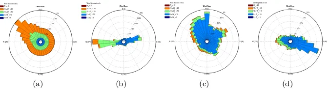
Figure 8: Wind distribution in test cases c-f. (a) case c (b) case d (c) case e (d) case f.
4.2. Experiments on WFLO
1) Test Cases. It is assumed that turbines are to be placed on a 2000m×2000m
405
wind farm. The occurrence of winds at the wind farm is described using wind roses, which show the strength, direction and frequency of winds. Six test cases are used to examine the performance of fGA. They are listed as follows: Case a The wind blows from one direction at a constant speed of 12m/s. Case b The wind has a constant speed of 12m/s and blows from one of 36
410
possible angles, which range from 0◦ to 350◦in increments of 10◦. The wind blows from each angle with an equal possibility.
Case c The wind blows from one of the 36 angles described above. Its speed takes three possible values, i.e., 8m/s, 12m/s, and 17m/s. The proba-bility distribution of wind speed and direction is visualized in Fig. 8(a).
415
Case d-f The wind direction and speed take the same values as those in Case c. The probability distribution of winds is visualized in Fig. 8(b), (c), (d) respectively.
2) Fitness evaluation. The goal of WFLO is to find a layout that maximizes the
power produced and minimizes the cost of wind turbines. The two objectives
420
can be combined into a single fitness value. Specifically, the fitness function is defined as the cost over the power [13]. Intuitively, this gives the cost of a unit of power.
3) Constraint handling. WFLO poses a restriction on the distance of two
de-ployed turbines. To avoid blade damage caused by turbulence, the distance
425
between any two turbines must be at least 5D, whereD is the rotor diameter. An individual may violate the constraint after the crossover and mutation op-erators. In the proposed fGA, the constraint is handled in a simple way. For the crossover operator, turbines in the crossover area of the first individual are first removed. Then, turbines in the crossover area of the second individual are
430
appended to the first individual one after another. If the introduction of a new turbine will cause violations, then the turbine is excluded. For the mutation operator, if the shift of a turbine will incur blade damage, then the shift is canceled.
Table 14: Notations in the formulation of WFLOP and their corresponding settings
Symbol Description Setting
rr Rotor radius 20 m
D Rotor diameter 40 m
z Hub height 60 m
z0 Surface roughness 0.3
CT Thrust coefficient 0.88
Table 15: Comparison of mean and best results obtained by the algorithms on case a
Algorithm Mean Best Wilcoxon test Fitness Turbines Cost Power Fitness Turbines cost Power G1 GA-WFLO 0.001401 41.74 28.508212 20343.53895 0.001388 44 29.838401 21501.7532 +
BPSO-TVAC 0.001373 42.98 29.229115 21284.06177 0.001372 42 28.650312 20880.72212 + G2 GPSO 0.001334 50 33.548447 25157.9356 0.001321 50 33.548447 25393.67349 + VNPSO 0.001334 50 33.548447 25157.61178 0.001324 50 33.548447 25338.51969 + G3 RS 0.001313 50 33.548447 25560.36256 0.001307 50 33.548447 25667.29586 + G4 GA-WMN 0.001307 52.83 35.360606 27045.58975 0.001305 53 35.466523 27170.7361 + fGA 0.001305 54.44 36.39942 27892.62157 0.001302 56 37.413 28730.32948 NA
4) Algorithms for comparison. The algorithms for comparison are grouped as
435
follows:
G1) GA-WFLO [34] and BPSO-TVAC [13]: Two grid-based methods, which divide the wind farm into 10×10 grids.
G2) GPSO and VNPSO: Two PSO algorithms using fixed-length encoding scheme.
440
G3) SA [57]: A recently proposed random search algorithm for the optimal placement of wind turbines.
G4) GA-WMN [53]: A genetic algorithm originally designed for the wireless mesh network planning problem. It is adapted here to tackle the WFLO problem.
445
5) Parameter setting. The notations of WFLO [3] and their corresponding
set-tings are listed in Table 14. The parameter setset-tings of fGA, GA-WMN, GPSO and VNPSO are the same as in RNP. GA-WFLO and BPSO-TVAC are set according to [34] and [13] respectively. The maximum number of turbines avail-able for placement is 100, i.e., Nmax = 100. The maximum number of fitness
450
evaluations is set to 100,000. Each algorithm is run 50 times for each test case.
6) Experimental results and discussion. Experimental results of the fGA and
the other four algorithms are reported in Tables 15-20. The Wilcoxon rank-sum test is utilized to see if there are significant differences between the results obtained by the fGA and other algorithms. Symbol ‘+’ in the last column
455
indicates the existence of significant difference. In addition, the convergence speed of the algorithms on the six cases are depicted in Fig. 9. The results are averaged over 50 runs.
Case a is a relatively simple case to handle, where the wind blows from one direction and the wind speed is constant. From Table 15, it can be seen that fGA
[image:19.612.128.487.222.294.2]Table 16: Comparison of mean and best results obtained by the algorithms on case b
Algorithm Mean Best Wilcoxon test Fitness Turbines Cost Power Fitness Turbines cost Power G1 GA-WFLO 0.001374 46.84 31.573646 22980.045 0.001371 47 31.668836 23103.1049 +
[image:20.612.135.482.261.331.2]BPSO-TVAC 0.001365 48.04 32.317633 23672.30818 0.001364 49 32.917108 24140.49174 + G2 GPSO 0.001348 50 33.548447 24887.24844 0.001343 50 33.548447 24979.37381 + VNPSO 0.001349 50 33.548447 24873.93534 0.001347 50 33.548447 24913.39712 + G3 RS 0.001357 50 33.548447 24722.52165 0.001349 50 33.548447 24876.17856 + G4 GA-WMN 0.001341 48.87 32.834979 24490.63152 0.001339 49 32.917108 24580.12842 + fGA 0.001336 50.02 33.562424 25116.08898 0.001334 50 33.548447 25141.2711 NA
Table 17: Comparison of mean and best results obtained by the algorithms on case c
Algorithm Mean Best Wilcoxon test Fitness Turbines Cost Power Fitness Turbines cost Power G1 GA-WFLO 0.001327 53.04 35.493836 26753.69232 0.001325 51 34.184054 25789.80437 +
[image:20.612.135.487.368.443.2]BPSO-TVAC 0.001322 52.02 34.836398 26358.00784 0.001321 52 34.823538 26361.36445 + G2 GPSO 0.001315 50 33.548447 25508.28371 0.001314 50 33.548447 25531.75912 + VNPSO 0.001315 50 33.548447 25503.70878 0.001315 50 33.548447 25516.99716 + G3 RS 0.001318 50 33.548447 25448.50594 0.001316 50 33.548447 25488.0407 + G4 GA-WMN 0.001311 54.57 36.48072 27835.29619 0.00131 55 36.761581 28059.74421 + fGA 0.001309 55.14 36.853073 28157.71249 0.001308 57 38.066615 29099.96617 NA
Table 18: Comparison of mean and best results obtained by the algorithms on case d
Algorithm Mean Best Wilcoxon test Fitness Turbines Cost Power Fitness Turbines cost Power G1 GA-WFLO 0.002401 45.27 30.611482 12750.41939 0.002388 46 31.052708 13001.4921 +
BPSO-TVAC 0.002365 49.27 33.086567 13990.14799 0.002361 50 33.548447 14207.30698 + G2 GPSO 0.00236 50 33.548447 14212.77597 0.002355 50 33.548447 14243.87585 + VNPSO 0.002361 50 33.548447 14209.34714 0.002355 50 33.548447 14245.45122 + G3 RS 0.002359 50 33.548447 14219.80587 0.002352 50 33.548447 14263.72354 + G4 GA-WMN 0.002346 50.9 34.121528 14546.73582 0.002343 52 34.823538 14860.43637 + fGA 0.002341 52.13 34.91032 14911.94289 0.002338 53 35.466523 15166.92009 NA
Table 19: Comparison of mean and best results obtained by the algorithms on case e
Algorithm Mean Best Wilcoxon test Fitness Turbines Cost Power Fitness Turbines cost Power G1 GA-WFLO 0.003136 48.53 32.626738 10403.66073 0.003131 50 33.548447 10716.1528 +
BPSO-TVAC 0.003115 49.5 33.232933 10667.72267 0.003113 50 33.548447 10775.76015 + G2 GPSO 0.003074 50 33.548447 10912.79427 0.003069 50 33.548447 10932.63723 + VNPSO 0.003074 50 33.548447 10913.36175 0.003067 50 33.548447 10936.83996 + G3 RS 0.00309 50 33.548447 10857.60784 0.00308 50 33.548447 10892.38847 + G4 GA-WMN 0.00306 50.1 33.613133 10984.15514 0.003057 49 32.917108 10767.5412 + fGA 0.003052 50.93 34.142456 11188.16839 0.003049 51 34.184054 11209.74475 NA
Table 20: Comparison of mean and best results obtained by the algorithms on case f
Algorithm Mean Best Wilcoxon test Fitness Turbines Cost Power Fitness Turbines cost Power G1 GA-WFLO 0.00313 46.3 31.242234 9981.177752 0.003122 44 29.838401 9558.727848 +
BPSO-TVAC 0.003088 48.67 32.709462 10592.60216 0.003082 50 33.548447 10883.93689 + G2 GPSO 0.003073 50 33.548447 10918.92088 0.003067 50 33.548447 10939.42207 + VNPSO 0.003073 50 33.548447 10915.91941 0.00307 50 33.548447 10928.76126 + G3 RS 0.003083 50 33.548447 10883.45863 0.003072 50 33.548447 10921.13958 + G4 GA-WMN 0.003056 50.13 33.634035 11006.25528 0.003053 50 33.548447 10987.32832 + fGA 0.003047 50.97 34.163914 11211.44176 0.003044 52 34.823538 11441.01969 NA
[image:20.612.136.484.482.552.2] [image:20.612.134.486.592.665.2]0 5 0 0 1 0 0 0 1 . 3 0
1 . 3 2 1 . 3 4 1 . 3 6 1 . 3 8 1 . 4 0 1 . 4 2 1 . 4 4 1 . 4 6 1 . 4 8 1 . 5 0 1 . 5 2 1 . 5 4 1 . 5 6
F
it
n
es
s
G e n e r a t i o n G A - WF L O B P S O - T V A C f G A G A - WM N G P S O R S V N P S O x 1 0- 3
(a)
0 5 0 0 1 0 0 0 1 . 3 3
1 . 3 4 1 . 3 5 1 . 3 6 1 . 3 7 1 . 3 8 1 . 3 9 1 . 4 0 1 . 4 1 1 . 4 2
x 1 0- 3
F
it
n
es
s
G e n e r a t i o n G A - WF L O B P S O - T V A C f G A G A - WM N G P S O R S V N P S O
(b)
0 5 0 0 1 0 0 0 1 . 3 0 8
1 . 3 1 0 1 . 3 1 2 1 . 3 1 4 1 . 3 1 6 1 . 3 1 8 1 . 3 2 0 1 . 3 2 2 1 . 3 2 4 1 . 3 2 6 1 . 3 2 8 1 . 3 3 0 1 . 3 3 2 1 . 3 3 4 1 . 3 3 6 1 . 3 3 8 1 . 3 4 0 x 1 0- 3
F
it
n
es
s
G e n e r a t i o n G A - WF L O B P S O - T V A C f G A G A - WM N P S O R S V N P S O
(c)
0 5 0 0 1 0 0 0 2 . 3 4
2 . 3 6 2 . 3 8 2 . 4 0 2 . 4 2 2 . 4 4 2 . 4 6 2 . 4 8 2 . 5 0 2 . 5 2 2 . 5 4
x 1 0- 3
F
ti
n
es
s
G e n e r a t i o n G A - WF L O B P S O - T V A C f G A G A - WM N G P S O R S V N P S O
(d)
0 5 0 0 1 0 0 0 3 . 0 4
3 . 0 5 3 . 0 6 3 . 0 7 3 . 0 8 3 . 0 9 3 . 1 0 3 . 1 1 3 . 1 2 3 . 1 3 3 . 1 4 3 . 1 5 3 . 1 6 3 . 1 7 3 . 1 8 3 . 1 9 3 . 2 0 x 1 0- 3
F
it
n
es
s
G e n e r a t i o n G A - WF L O B P S O - T V A C f G A G A - WM N G P S O R S V N P S O
(e)
0 5 0 0 1 0 0 0 3 . 0 4
3 . 0 6 3 . 0 8 3 . 1 0 3 . 1 2 3 . 1 4 3 . 1 6 3 . 1 8 3 . 2 0 3 . 2 2 3 . 2 4 x 1 0- 3
F
it
n
es
s
G e n e r a t i o n G A - W F L O B P S O - T V A C f G A G A - W M N G P S O R S V N P S O
[image:21.612.139.476.135.337.2](f)
Figure 9: Convergence performance of the algorithms on WFLO cases. (a) case a (b) case b (c) case c (d) case d (e) case e (f) case f.
achieves the best fitness value with a reasonably large number of turbines. The performance of GA-WMN and RS is slightly worse than that of fGA. GPSO and VNPSO perform virtually the same. In comparison, the performance of the two grid-based methods (GA-WFLO and BPSO-TVAC) is in some ways unsatisfactory.
465
In case b, the average number of turbines obtained by the fGA is 50.02 (reported in Table 16), which is very close to Nmax/2. In this case, it is con-sidered that the methods based on the fixed-length encoding scheme are seen in their best trials, because they are completely free from the task of adjusting the number of turbines and the deficiency is eliminated. However, even though
470
GPSO and VNPSO have a head-start, they are still outperformed by fGA in all 50 runs. The superiority of the fGA owes much to the subarea-swap crossover, which offers a natural way to adjust the number of turbines and at the same time greatly enhance the search ability. The crossover areas are self-adapted according to the distribution of nodes and are therefore more conducive to
evo-475
lution. In comparison, the two grid-based methods fail to catch up with GPSO, VNPSO, RS, GA-WMN, and fGA.
Compared to the previous two cases, test cases c-f are more practical and complicated. From Tables 17-20, it can be seen that fGA yields the best results among all algorithms. The average number of turbines used by the fGA is
480
out to be very promising.
485
To summarize, in all the six cases of WFLO, the fGA performs the best, followed by GA-WMN, RS, GPSO and VNPSO. In comparison, the perfor-mance of the two grid-based methods (GA-WFLO and BPSO-TVAC) is not as good as the fGA. This is mainly due to that, in the grid-based algorithms, the optimization of the positions of nodes is coarse-grained. As the positions for
490
placement are confined to the center of each grid, grid-based methods cannot make the most of the wind farm space. In contrast, fGA, GPSO, and VNPSO are free from this restriction and are able to explore the wind farm completely and thoroughly, leading to more competitive results.
Overall, experimental results on RNP and WFLO reveal the drawbacks of
495
previous methods. 1) Grid-based methods are lack of flexibility and are unable to simultaneously optimize the attached properties of nodes. 2) The perfor-mance of GPSO and VNPSO can only be guaranteed on the premise that the predefined number of nodes is close to the suitable number. In contrast, the fGA yields relatively good results in both RNP and WFLO. From the experimental
500
results, it can be seen that the fGA is able to automatically adjust the number of nodes and optimize nodes positions and attached properties simultaneously. Its flexibility and efficiency make it a very promising approach for solving different kinds of NPPs.
4.3. Experiments on the Primitive Coverage Problem 505
To show the advantage of the proposed algorithm over the existing GA-based node placement approaches, experiments are conducted on a primitive NPP called “coverage problem”. The problem is formulated as follows. There are many objects scattered in a working area. The task is to place a number of nodes in the area to cover the objects. Each node has a fixed sensing range. An
510
object is said to be covered by a node if it is in the sensing range of the node. The optimization goal is to cover all the objects by using the least number of nodes. Nine randomly generated test cases are used in the experiment to test the performance of fGA,GA-WMN [53], GA-WFLO [34], and VNPSO-RNP [12]. For each test case, 100 objects are scattered randomly in a 100m×100m square
515
area. The sensing radius of nodes is fixed at 10m. The maximum number of fitness evaluations is set to 400,000. The mean results of the algorithms over 50 independent runs are summarized in Table 21. From the table, it can be seen that fGA is able to achieve a 100% coverage rate in all the test cases and the number of deployed nodes is less than those of the other three algorithms. This
520
is attributed to the dynamic feature introduced by the crossover operator, which helps the algorithm to focus its attention on the critical region of the working area. Compared with fGA, the performance of GA-WMN and GA-WFLO is in some sense unsatisfactory. GA-WMN fails to realize full coverage in two of the test cases, while GA-WFLO consumes a larger number of nodes.
525
4.4. Parameter Investigation
To study the influence of the crossover and mutation probabilities, experi-ments are conducted on the WFLO problem using different settings ofPc and
Table 21: Comparison of mean results obtained by the algorithms on the coverage problem
Test cases fGA GA-WMN GA-WFLO VNPSO-RNP
Coverage No. nodes Coverage No. nodes Coverage No. nodes Coverage No. nodes Case a 100.00% 24.27 99.97% 25.80 100.00% 37.37 100.00% 31.93 Case b 100.00% 22.90 100.00% 24.47 100.00% 32.30 100.00% 30.50 Case c 100.00% 22.73 100.00% 24.50 100.00% 33.07 100.00% 31.37 Case d 100.00% 20.30 100.00% 23.13 100.00% 31.70 100.00% 28.93 Case e 100.00% 22.10 100.00% 24.27 100.00% 34.10 100.00% 31.10 Case f 100.00% 22.60 100.00% 24.93 100.00% 35.13 100.00% 30.03 Case g 100.00% 22.27 99.93% 24.47 100.00% 35.17 100.00% 30.23 Case h 100.00% 24.23 100.00% 25.93 100.00% 35.37 100.00% 31.80 Case i 100.00% 22.10 100.00% 24.30 100.00% 34.37 100.00% 30.13
0 . 1 0 . 2 0 . 3 0 . 4 0 . 5 0 . 6 0 . 7 0 . 8 0 . 9 3 . 0 4 2
3 . 0 4 4 3 . 0 4 6 3 . 0 4 8 3 . 0 5 0 3 . 0 5 2 3 . 0 5 4 3 . 0 5 6 3 . 0 5 8 3 . 0 6 0 3 . 0 6 2
F
it
n
es
s
P c
x1 0-3
(a)
0 . 0 1 0 . 0 2 0 . 0 3 0 . 0 4 0 . 0 5 0 . 0 6 0 . 0 7 0 . 0 8 0 . 0 9 0 . 1 3 . 0 3 6
3 . 0 3 8 3 . 0 4 0 3 . 0 4 2 3 . 0 4 4 3 . 0 4 6 3 . 0 4 8 3 . 0 5 0 3 . 0 5 2 3 . 0 5 4 3 . 0 5 6 3 . 0 5 8 3 . 0 6 0
P m
x1 0-3
F
it
n
es
s
(b)
Figure 10: Effect of the parameter settings. (a)Pc(b)Pm.
Pm. Specifically, the value ofPcranges from 0.1 to 0.9. As forPm, values in the interval [0.01, 0.1] are tested. We first investigate the effect ofPc. When study-530
ing the influence ofPc,Pmis fixed at 0.1. Subsequently, when testing the effect
ofPm,Pc is fixed at 0.9. Experimental results on the test case f are presented
in Fig. 10 using box plots. From the figure, it can be observed that fGA with the setting Pc = 0.9 is able to achieve the best fitness value. In comparison, fGA is not very sensitive to the setting ofPm. A value between 0.01 and 0.1 is
535
able to provide very stable performance.
5. Conclusion and Future Work
In this paper, we introduce a general framework of node placement prob-lems (NPPs). Further, a flexible algorithm termed fGA is developed to tackle different kinds of NPPs. Compared to the existing approaches, the fGA has
540
several notable features. First, a variable-length encoding scheme is incorporat-ed to enable the automatic adjustment of the number of nodes deployincorporat-ed in the working area. Second, by employing a novel subarea-swap crossover, the fGA is capable of adjusting the number and properties of nodes simultaneously in a natural and efficient manner. For further flexibility, a Gaussian mutation is
545
Experiments have been carried out on two typical NPPs, i.e., RFID net-work planning and wind farm layout optimization problems, to investigate the performance of the proposed algorithm. The experimental results show that
550
fGA outperforms existing algorithms using a grid-based method or a fix-length method. In dealing with the WFLO problem, fGA is able to find the best fitness values among the compared algorithms. As for the RNP problem, fGA manages to obtain layouts with 100% coverage rates by using the least number of reader-s. Meanwhile, the layouts produced by fGA also involve lower interference and
555
consume less power than the layouts produced by other algorithms. The results on the two problems reveal that fGA is a promising tool for solving NPPs.
In future research, it would be interesting to apply the fGA to a wider va-riety of NPPs to further investigate its applicability. According to the 2-D representation scheme, it is noteworthy that the fGA can be adapted to
tack-560
le three-dimensional node placement problems, which have received increasing attention in recent years. Moreover, as some NPPs have multiple conflicting objectives, there is a desire to incorporate the fGA with multi-objective opti-mization techniques to handle multi-objective NPPs.
References
565
[1] Q. Guan, Y. Liu, Y. Yang, W. Yu, Genetic approach for network planning in the RFID systems, in: Intelligent Systems Design and Applications, 2006. ISDA’06. Sixth International Conference on, volume 2, IEEE, 2006, pp. 567–572.
[2] M. Younis, K. Akkaya, Strategies and techniques for node placement in
570
wireless sensor networks: A survey, Ad Hoc Networks 6 (2008) 621–655. [3] M. Samorani, The wind farm layout optimization problem, in: Handbook
of Wind Power Systems, Springer, 2013, pp. 21–38.
[4] B. Guyaguler, R. Horne, Optimization of well placement, Journal of Energy Resources Technology 122 (2000) 64–70.
575
[5] A. Konstantinidis, K. Yang, Q. Zhang, D. Zeinalipour-Yazti, A multi-objective evolutionary algorithm for the deployment and power assignment problem in wireless sensor networks, Computer networks 54 (2010) 960– 976.
[6] E. L. Lloyd, G. Xue, Relay node placement in wireless sensor networks,
580
Computers, IEEE Transactions on 56 (2007) 134–138.
[7] Y. T. Hou, Y. Shi, H. D. Sherali, S. F. Midkiff, On energy provisioning and relay node placement for wireless sensor networks, Wireless Commu-nications, IEEE Transactions on 4 (2005) 2579–2590.
[8] J. Tang, B. Hao, A. Sen, Relay node placement in large scale wireless
585
sensor networks, Computer communications 29 (2006) 490–501.
[9] H. Chen, Y. Zhu, RFID networks planning using evolutionary algorithms and swarm intelligence, in: Wireless Communications, Networking and Mobile Computing, 2008. WiCOM’08. 4th International Conference on, IEEE, 2008, pp. 1–4.
590
[10] I. Bhattacharya, U. K. Roy, Optimal placement of readers in an RFID net-work using particle swarm optimization, International Journal of Computer Networks & Communications 2 (2010) 225–234.
[11] H. Chen, Y. Zhu, K. Hu, T. Ku, RFID network planning using a multi-swarm optimizer, Journal of Network and Computer Applications 34 (2011)
595
888–901.
[12] Y.-J. Gong, M. Shen, J. Zhang, O. Kaynak, W.-N. Chen, Z.-H. Zhan, Optimizing RFID network planning by using a particle swarm optimization algorithm with redundant reader elimination, Industrial Informatics, IEEE Transactions on 8 (2012) 900–912.
600
[13] S. Pookpunt, W. Ongsakul, Optimal placement of wind turbines with-in wwith-ind farm uswith-ing bwith-inary particle swarm optimization with time-varywith-ing acceleration coefficients, Renewable Energy 55 (2013) 266–276.
[14] Y. Ero˘glu, S. U. Se¸ckiner, Wind farm layout optimization using particle filtering approach, Renewable Energy 58 (2013) 95–107.
605
[15] Y. Chen, H. Li, K. Jin, Q. Song, Wind farm layout optimization using ge-netic algorithm with different hub height wind turbines, Energy Conversion and Management 70 (2013) 56–65.
[16] B. P´erez, R. M´ınguez, R. Guanche, Offshore wind farm layout optimization using mathematical programming techniques, Renewable Energy 53 (2013)
610
389–399.
[17] B. Guyaguler, R. N. Horne, et al., Uncertainty assessment of well placement optimization, in: SPE annual technical conference and exhibition, Society of Petroleum Engineers, 2001, pp. 1–13.
[18] W. Bangerth, H. Klie, V. Matossian, M. Parashar, M. F. Wheeler, An
au-615
tonomic reservoir framework for the stochastic optimization of well place-ment, Cluster Computing 8 (2005) 255–269.
[19] W. Bangerth, H. Klie, M. Wheeler, P. Stoffa, M. Sen, On optimization algorithms for the reservoir oil well placement problem, Computational Geosciences 10 (2006) 303–319.
620
[21] J. Wang, N. Zhong, Efficient point coverage in wireless sensor networks, Journal of Combinatorial Optimization 11 (2006) 291–304.
625
[22] P. Fagerfj¨all, Optimizing wind farm layout: more bang for the buck using mixed integer linear programming, Master’s thesis, Chalmers University of Technology, Gothenburg University, Gothenburg, Sweden, 2010.
[23] S. Donovan, An improved mixed integer programming model for wind farm layout optimisation, in: Proceedings of the 41st Annual Conference of the
630
Operations Research Society, 2006, pp. 143–151.
[24] M. Nandigam, S. K. Dhali, Optimal design of an offshore wind farm layout, in: Power Electronics, Electrical Drives, Automation and Motion, 2008. SPEEDAM 2008. International Symposium on, IEEE, 2008, pp. 1470–1474.
[25] K. Kar, S. Banerjee, Node placement for connected coverage in sensor
635
networks, in: WiOpt’03: Modeling and Optimization in Mobile, Ad Hoc and Wireless Networks, 2003, pp. 1–2.
[26] W.-C. Ke, B.-H. Liu, M.-J. Tsai, Constructing a wireless sensor network to fully cover critical grids by deploying minimum sensors on grid points is np-complete, IEEE Transactions on Computers 56 (2007) 710–715.
640
[27] R.-S. Ko, The complexity of the minimum sensor cover problem with unit-disk sensing regions over a connected monitored region, International Journal of Distributed Sensor Networks 2012 (2011) 1–25.
[28] L. Davis, Handbook of genetic algorithms, Bristol and Oxford University Press, 1991.
645
[29] Y.-J. Gong, W.-N. Chen, Z.-H. Zhan, J. Zhang, Y. Li, Q. Zhang, J.-J. Li, Distributed evolutionary algorithms and their models: A survey of the state-of-the-art, Applied Soft Computing 34 (2015) 286–300.
[30] J. Kennedy, J. F. Kennedy, R. C. Eberhart, Y. Shi, Swarm intelligence, Morgan Kaufmann, 2001.
650
[31] B. Saavedra-Moreno, S. Salcedo-Sanz, A. Paniagua-Tineo, L. Prieto, A. Portilla-Figueras, Seeding evolutionary algorithms with heuristics for optimal wind turbines positioning in wind farms, Renewable Energy 36 (2011) 2838–2844.
[32] A. P. Bhondekar, R. Vig, M. L. Singla, C. Ghanshyam, P. Kapur, Genetic
655
algorithm based node placement methodology for wireless sensor network-s, in: Proceedings of the international multiconference of engineers and computer scientists, volume 1, Citeseer, 2009, pp. 18–20.
[33] G. Mosetti, C. Poloni, B. Diviacco, Optimization of wind turbine position-ing in large windfarms by means of a genetic algorithm, Journal of Wind
660
Engineering and Industrial Aerodynamics 51 (1994) 105–116.