City, University of London Institutional Repository
Citation:
Schroth, E., Suarez, G. A. & Taylor, L. A. (2014). Dynamic debt runs and
financial fragility: Evidence from the 2007 ABCP crisis. Journal of Financial Economics,
112(2), pp. 164-189. doi: 10.1016/j.jfineco.2014.01.002
This is the draft version of the paper.
This version of the publication may differ from the final published
version.
Permanent repository link:
http://openaccess.city.ac.uk/14004/
Link to published version:
http://dx.doi.org/10.1016/j.jfineco.2014.01.002
Copyright and reuse: City Research Online aims to make research
outputs of City, University of London available to a wider audience.
Copyright and Moral Rights remain with the author(s) and/or copyright
holders. URLs from City Research Online may be freely distributed and
linked to.
Other uses, including reproduction and distribution, or selling or
licensing copies, or posting to personal, institutional or third party
websites are prohibited.
In most cases authors are permitted to post their version of the
article (e.g. in Word or Tex form) to their personal website or
institutional repository. Authors requiring further information
regarding Elsevier’s archiving and manuscript policies are
encouraged to visit:
Dynamic debt runs and financial fragility: Evidence from
the 2007 ABCP crisis
$Enrique Schroth
a, Gustavo A. Suarez
b, Lucian A. Taylor
c,naCass Business School, City University, London, United Kingdom bFederal Reserve Board, United States
cWharton School, University of Pennsylvania, United States
a r t i c l e i n f o
Article history:
Received 6 December 2012 Received in revised form 26 July 2013
Accepted 22 August 2013 Available online 31 January 2014
JEL classification:
G01 G21 G28
Keywords:
Runs
Financial crises Structural estimation
Asset-backed commercial paper
a b s t r a c t
We use the 2007 asset-backed commercial paper (ABCP) crisis as a laboratory to study the determinants of debt runs. Our model features dilution risk: maturing short-term lenders demand higher yields in compensation for being diluted by future lenders, making runs more likely. The model explains the observed tenfold increase in yield spreads leading to runs and the positive relation between yield spreads and future runs. Results from structural estimation show that runs are very sensitive to leverage, asset values, and asset liquidity, but less sensitive to the degree of maturity mismatch, the strength of guarantees, and asset volatility.
&2014 The Authors. Published by Elsevier B.V. This is an open access article under the CC
BY license (http://creativecommons.org/licenses/by/3.0/).
Contents lists available atScienceDirect
journal homepage: www.elsevier.com/locate/jfec
Journal of Financial Economics
http://dx.doi.org/10.1016/j.jfineco.2014.01.002
0304-405X&2014 The Authors. Published by Elsevier B.V. This is an open access article under the CC BY license
(http://creativecommons.org/licenses/by/3.0/).
☆This paper has benefited from suggestions by Zhiguo He (the referee), Rui Albuquerque, Franklin Allen, Carlos Castro, Shawn Cole, Itay Goldstein, Carole
Gresse (discussant), Jungsuk Han (discussant), Julien Hugonnier, Wei Jiang (discussant), Jonathan Karpoff (discussant), Anna Kovner (discussant), Bo Larson (discussant), Semyon Malamud, Konstantin Milbradt, Afrasiab Mirza (discussant), Erwan Morellec (discussant), Greg Nini, Martin Oehmke, Asani Sarkar (discussant), Philipp Schnabl, Jose Tessada (discussant), and Toni Whited (discussant); seminar participants at Drexel University, Erasmus University, HEC Paris, London Business School, London School of Economics, MIT, Tilburg University, the Universities of Alberta, Pittsburgh, Virginia, Washington, and Wisconsin; the Wharton School of Business, the 2012 Fifth Financial Risks International Forum, the 2012 Paris Spring Corporate Finance Conference, the 2012 European Finance Association Meetings, the 2012 European Summer Symposium in Finance (Gerzensee), the 2013 Financial Intermediation Research Society Conference, the 2012 Frontiers of Finance Conference (Warwick), the 2013 Western Finance Association Meetings, the 2012 Wharton Conference on Liquidity and Financial Crises, the 2012 UBC Winter Finance Conference, and the 2013 UC International Finance Conference. Schroth and Taylor gratefully acknowledge financial support provided by the Sloan Foundation grant to the Wharton Financial Institutions Center. Scott Aubuchon and Qiwei Shi provided excellent research assistance. All views expressed in this paper are ours and not necessarily those of the Federal Reserve System or its Board of Governors.
nCorresponding author.
1. Introduction
Debt runs played a central role in the financial crisis of 2007–2008. Investors ran on asset-backed commercial
paper (ABCP) starting in August 2007, on repo starting in September 2007, and on money market mutual funds in September 2008. Investors also ran on some large banks such as Northern Rock (September 2007) and Bear Stearns (March 2008).1
These events have reignited the debate about what causes runs and how we can prevent them. We contribute to this debate by measuring the sensitivity of runs to several contributing factors, including maturity mismatch, leverage, asset volatility and liquidity, and the strength of guarantees. The results help answer four questions that are vital to policy makers, regulators, bankers, and investors: How fragile are financial intermediaries? How can we design financial intermediaries ex ante to control the risk of future runs? What are the warning signs that a run is imminent? Finally, which interventions best prevent runs ex post once conditions have started deteriorating?
We address these questions by estimating a structural model of debt runs using data from the 2007 ABCP crisis. ABCP issuers, commonly referred to as conduits, are off-balance sheet investment vehicles that banks structure to invest in pools of medium- and long-term assets such as trade receivables and mortgage-backed securities (MBS).2
A conduit finances these investments by issuing short-term ABCP to dispersed creditors and rolling it over until the conduit chooses to stop investing. The bank sponsor-ing the conduit provides some form of guarantee in the event that the conduit can no longer roll over its debt.
The amount of ABCP outstanding in the U.S. contracted by $370 billion (roughly one-third) between August and December of 2007. Several authors have interpreted this event as a run on debt.3In a debt run, creditors refuse to
roll over their debt if they fear that other creditors will not roll over, in some cases even if the borrower is solvent. In the case of ABCP, roughly 40% of conduits had stopped rolling over maturing debt by the end of 2007.
ABCP provides a useful laboratory to study financial fragility for four reasons. First, since ABCP conduits per-form maturity transper-formation, they are representative of many other financial intermediaries. Second, the simple balance sheet and operating structure of ABCP conduits lend themselves to modeling. Third, we have detailed data on the yield, maturity, size, and issuer's identity for all U.S. ABCP transactions in 2007. Because yields adjust at each
maturity date, their time series measures the conduit's health continuously and can potentially be an important lead indicator of runs. Finally, as Krishnamurthy, Nagel,
and Orlov (2014)argue, the ABCP crisis was important in
itself:
The contraction in both repo and ABCP are consistent with the views of many commentators that a contrac-tion in the short-term debt of shadow banks played an important role in the collapse of the shadow banking sector. However, it is important to note that the ABCP plays a more important role than repo in this regard.
In fact, runs on ABCP could have had a broad effect on financial intermediation through two channels. First, runs impaired ABCP conduits' ability to fund assets such as trade receivables or student loan receivables. Second, the runs on ABCP conduits forced their sponsoring banks to take troubled assets like mortgage securities back onto their own books, which impaired lending to nonfinancial firms and ultimately harmed economic activity (Irani, 2011).
Our model of ABCP conduits is based onHe and Xiong (2012a). A conduit finances a long-term asset using short-term, dispersed debt with overlapping maturities. Cred-itors track the asset's value and optimally run as soon as the conduit's leverage crosses above an endogenous threshold. A creditor's decision to run depends on chan-ging expectations that other creditors will run. We extend
He and Xiong's (2012a)model so that debt yields are not
fixed but instead vary endogenously over time, so as to make lenders indifferent between rolling over or not. This extension is necessary: we show empirically that yields on ABCP forecast runs, and yields increase exponentially leading up to runs. To have any chance of fitting these data, the model must make predictions about the time series of yields.
The model's parameters include the debt's maturity; the perceived strength of the sponsor's guarantee; and the asset's volatility, maturity, and liquidation discount in default. We observe some of these parameters directly in the data, and we estimate others using the simulated method of moments (SMM).
We find three main results. First, we show that runs are very sensitive to leverage and asset liquidity, but are less sensitive to the degree of maturity mismatch, asset vola-tility, and perceived guarantee strength. We measure these sensitivities by comparing simulated run probabilities between our estimated model and a counterfactual model with altered parameter values. We measure these sensi-tivities in both the early and late stages of a simulated crisis. In the late stages, increasing the asset's liquidation recovery rate by 1% (from 92.0% to 92.9%), while holding all else equal, lowers the probability of a run within three months from 70% to 39%. Decreasing the conduit's lever-age by 1% (from 91.4% to 90.4%) has an almost identical impact. In contrast, reducing the run probability by the same amount would require either reducing asset volati-lity by 40%, increasing average debt maturity by 190%, reducing average asset maturity by 98%, or increasing the guarantee's expected life span by 413%.
1Brunnermeier (2009) andKrishnamurthy (2009)summarize the
events of 2007–2008. We discuss the literature on ABCP below.Gorton
and Metrick (2012)andKrishnamurthy, Nagel, and Orlov (2014)
empiri-cally investigate the run on repo.Martin, Skeie, and Von Thadden (2012)
provide a model of repo runs.Kacperczyk and Schnabl (2013)examine
the run on money market funds.
2One prevalent view is that ABCP conduits were essentially a way for
sponsoring banks to take on systemic risk beyond regulations, without
transferring the risk to ABCP investors. See Acharya and Richardson
(2009),Acharya and Schnabl (2010),Acharya, Schnabl, and Suarez (2013),
Brunnermeier (2009), andShin (2009).
3See, for instance,Covitz, Liang, and Suarez (2013),Acharya, Schnabl,
These results shed light on how regulators and bankers can manage the risk of runs, both when forming new conduits and during a crisis. For example, crisis management policies with modest effects on asset liquidity (e.g., purchas-ing distressed assets) or conduit leverage (e.g., injectpurchas-ing equity) can have substantial effects on the likelihood of runs. High ABCP yields, which result from deteriorating funda-mentals, are a warning sign that a run is imminent. The model provides a quantitative mapping between these warning signs and the likelihood of runs. Of course, we do not address the feasibility or the cost of policy interventions, nor do we analyze how changing one fundamental (e.g., liquidity) could affect another (e.g., debt maturity).
The second main result is that the model can fit several features of the 2007 ABCP crisis. The model explains 73% of the sharp decline in total ABCP outstanding in the second half of 2007. For conduits offering weak guarantees to investors (‘Structured investment vehicle’ (SIV) and ‘Extendible notes’), the model comes quite close to fitting the magnitude and timing of the dramatic run-up in yields before runs, the overall level of ABCP yield volatility and its relation to yield levels, and the relatively high likelihood that conduits recover from a run. In both simulated and actual data, the current yield level helps forecast whether a run will occur. The model's main shortcoming is that, for conduits offering strong guarantees (‘Full credit’ or ‘Full liquidity’), it overpredicts runs when yields are high.
Our third result is theoretical. We show that introdu-cing time-varying yields into the model typically makes runs more likely, relative toHe and Xiong's (2012a)model with constant, exogenous yields. Using He and Xiong's (2012a)calibrated parameter values, we find that runs are 1.3–51 times more likely in our model than theirs. The
reason, as He and Xiong (2012a) conjecture, is that the conduit must offer high yields to induce rollover when conditions deteriorate. These high yields dilute all out-standing debt that matures later. Creditors preemptively demand higher yields in compensation for the risk of future dilution. These higher yields in turn make leverage build up faster, which makes runs more likely. This new risk, which we call ‘dilution risk,' can be an important
driver of yields and runs.
Several papers measure the determinants of runs using a reduced-form approach. Covitz, Liang, and Suarez (2013)
show that runs on ABCP conduits are negatively related to the strength of their guarantees.Calomiris and Mason (1997,
2003)show that bank runs during the Great Depression are
correlated with measures of bank solvency and shocks to the aggregate, regional, and local economies. Using data on an Indian bank, Iyer and Puri (2012) show that runs are positively related to weaker deposit insurance, a shorter or shallower relationship with the bank, and runs by one's peers.Chen, Goldstein, and Jiang (2010)provide evidence of strategic complementarities in mutual funds.
We depart from the existing empirical literature by taking a structural estimation approach. The structural approach complements the reduced-form approach by overcoming certain data limitations and by imposing diffe-rent identifying assumptions. The reduced-form approach requires data on the determinants of runs, many of which are difficult to obtain in the ABCP setting. For example,
data on conduit leverage and asset holdings are not publicly available.4We overcome this limitation by
struc-turally estimating several run determinants. The reduced-form approach also requires a data set with sufficient variation in the determinants of runs. Finding variation is potentially a challenge in the ABCP setting because con-duits resemble each other on many dimensions. The structural approach requires no heterogeneity in these determinants, as we use counterfactual analysis to mea-sure the sensitivity of runs to their various determinants. Both approaches impose strong identifying assumptions. The reduced-form approach assumes we have exogenous variation in the determinants of runs, which is difficult to find. The structural approach assumes that the model is true. Therefore, our exercise is not meant to identify coordination failures over any alternative mechanism for the sharp decline in ABCP. However, the structural approach allows us to show that a model of coordination failures can quantitatively and jointly fit several features of the data. This paper therefore takes a step toward provid-ing a quantitative model of financial fragility, which is crucial for guiding the management and regulation of financial intermediaries.
The paper is structured as follows.Section 2describes the model's assumptions and solution.Section 3discusses its predictions regarding dilution risk and the likelihood of runs.Section 4describes the data, identification, and SMM estimation.Section 5assesses model fit and describes our parameter estimates.Section 6uses the estimated model to explore the determinants of runs, Section 7 discusses policy implications, andSection 8concludes.
2. The model
We extend the model of He and Xiong (2012a) by allowing yields on short-term debt to adjust over time in response to changes in fundamentals. All assumptions below are shared with He and Xiong (2012a) unless otherwise noted.Appendix Adescribes the solution.
The model includes several features of ABCP conduits. The conduit finances a long-term asset using short-term, dispersed debt with overlapping maturities. The conduit must roll over this debt several times before the conduit ends, so the conduit faces rollover risk. The conduit's sponsor provides imperfect credit support if the conduit cannot roll over its paper.
2.1. Assumptions
2.1.1. Asset
At time zero, an ABCP conduit purchases a long-horizon asset. This asset represents the portfolio of assets a conduit typically buys. For the overall ABCP industry in 2007, the largest assets classes were trade receivables (14%), credit cards (12%), auto loans (11%),‘securities’(11%), commercial
4Even if asset holdings were known, measuring asset liquidity is
loans (10%), and mortgage-related assets (9%).5 The
con-duit reinvests any interim cash flows from the asset. For example, the conduit could buy new trade receivables using the payouts from maturing receivables. The conduit therefore makes no net interim payouts to investors.6The
asset produces a single net payout when the conduit matures, meaning the conduit winds down operations. The conduit matures randomly and independently at a time τϕ that arrives according to a Poisson process with
intensityϕ, so the conduit's expected time until maturity is always 1=ϕ. At maturity, the asset produces a payoutyτϕ,
whereyfollows a geometric Brownian motion with driftμ and volatilitys:
dyt
yt ¼μdtþsdZt: ð1Þ
Agents observeytat all times. All agents in the economy are risk neutral and have discount rate ρ, so the asset's value at timetis
F y! "t %Et e& ðτϕ&tÞρyτϕ
h i
¼ρ ϕ
þϕ&μyt: ð2Þ
2.1.2. Debt financing
The conduit finances the asset by initially borrowing $1 from a continuum of short-term creditors. Consistent with industry practice, the conduit also issues equity to its sponsor. The conduit's debt is zero-coupon and has endogenous face valueRtper dollar loaned at datet. In contrast, debt contracts
inHe and Xiong (2012a)have face value normalized to one
and offer exogenous interest rater. Each debt contract in our model matures randomly and independently with probability δdt in the interval½t;tþdt(, implying that a debt contract's
average remaining maturity always equals 1/δ. This modeling device, which follows Calvo (1983), Blanchard (1985), and
Leland (1998), reflects that ABCP conduits deliberately spread their debt maturities over time to reduce funding liquidity risk. These assumptions capture an important feature of the ABCP market, which is that before a given lender's debt matures, other lenders' debt will mature and potentially fail to roll over. Our assumptions imply that the conduit rolls over a fractionδdtof its debt every instant, and the total face value of debt,Dt, fluctuates over time according to
dDt¼δDtðRt&1Þdt: ð3Þ
2.1.3. Runs, liquidation, and the sponsor's guarantee
As payment for a maturing loan, lenders accept a new loan with a potentially different face value. If lenders choose not to roll over, we say that they run. We assume lenders roll over if they are indifferent between rolling
over and running. If lenders run and the conduit cannot raise funds to pay off maturing lenders, then the conduit defaults. In default, the conduit sells the asset at a fraction αof its fair market price, which yieldsLðytÞ %αFðytÞ.
Parameter α measures the asset's liquidity in the run state.7Equivalently,αis the asset's recovery rate in default.
Consistent with industry practice, the conduit distributes bankruptcy proceeds LðytÞ to outstanding creditors pro
rata, i.e., in proportion to their face value.
An ABCP conduit's sponsor provides a guarantee, which is typically a line of credit the conduit can use if it is unable to issue new paper.Section 4.1describes the four types of guarantee in use in 2007. We followHe and Xiong (2012a)
by modeling guarantees as an imperfect credit line from the sponsor. If the conduit experiences a run, it pays off maturing paper by borrowing from the sponsor at the prevailing rollover yield and maturity. The credit line therefore allows the conduit to potentially survive a run long enough for the conduit to recover and begin issuing paper again. We assume the credit line fails independently, causing default, each instant with probabilityθδdt. Once a run starts, the credit line is expected to last for 1=ðθδÞ
years, so conduits with higher values of θ have weaker guarantees.
2.2. ABCP pricing
We typically work with yield spreads, denoted rt(in units of fraction per year), which we can compute from face valuesRt(in units of dollars) using8
rt¼ ðRt&1Þ ) ðϕþδÞ&ρ: ð4Þ
Unlike in He and Xiong (2012a), debt is priced in a competitive market so that creditors exactly break even. This pricing assumption makes the debt we study here identical to the one in Leland and Toft (1996), Leland (1998), and the short-term class inHe and Xiong (2012b). Specifically, the conduit sets its rollover yield spreadrtso that if creditors loan the conduit $1 at timet, they receive a debt contract worth $1. Intuitively, if times are bad, the conduit must issue paper at a high yield spreadrtto make creditors break even. If times are good, the new paper is almost risk free, and the new rollover yield will be close to the risk-free rate.
We assume the conduit cannot or will not issue debt with a yield spread above an exogenous cap,r. This is an important assumption, which, as we show later, implies that creditors run exactly when the spread hits its cap. There are a several rationales for assuming yield spreads cannot go to infinity as conditions worsen.
5Data are from‘The ABC's of ABCP,’an unpublished document from
Societe Generale. Reported portfolio weights are measured on August 31,
2007. The ambiguous‘securities’category could include mortgage-related
securities.
6InHe and Xiong (2012a), the asset pays a fixed dividend, which the
conduit uses to pay a coupon on the bond. Our model assumes zero-coupon debt, since commercial paper is a discount security that pays face value at maturity with no interim coupons.
7Note that we do not assume that asset liquidity is constant. Instead,
we assume that the creditors' expected asset liquidation valuein the run
state, i.e., if the whole asset is sold to pay off running creditors, is constant.
8The yield spreadr
tis the interest rate (in excess of the risk-free rate,
ρ) that delivers the same value as a zero-coupon bond with face valueRt,
under the assumption that both bonds are paid back in full at
τ¼minðτδ;τϕÞ. Eq.(4)follows from the condition
Et
Zτ
t e &ρðs&tÞ
ðρþrtÞdsþe&ρðτ&tÞ
# $
One rationale relates to institutional constraints. The main investors in ABCP are money market funds, which are required to invest mainly in assets with very high ratings (e.g., A-1 by Standard and Poor's (S&P) or P-1 by Moody's).9 As an ABCP conduit's health declines and its
rollover yields rise, eventually the conduit will lose its A-1/ P-1 rating and its creditors will be unable to roll over its paper. Effectively, the conduit will be unable to roll over paper once yield spreads reach a certain level, i.e., a cap.
Credit rationing, as in Stiglitz and Weiss (1981), pro-vides another rationale for capping yields. Once yield spreads exceed some level, only the conduits with very risky assets will be willing to roll over their paper. Because of this adverse selection problem, creditors will refuse to accept yield spreads above this cap.
In these first two rationales, it is creditors who walk away from the conduit in a run. There is another rationale in which the sponsor walks away. If conditions worsen enough, rollover yields become so high that the ABCP conduit's equity is very low. The sponsor then has little incentive to keep operating the conduit. As in Leland
(1998), where the default boundary is chosen to maximize
the value of equity at default, the sponsors can choose the run threshold indirectly via the yield cap.10
A final rationale is that without a cap on yields, we find no runs. We cannot prove this result generally since we lack closed-form solutions, but for empirically relevant parameter values we show that the predicted probability of a run goes to zero asr gets large (Fig. 8). Intuitively, a higher yield cap incentivizes rollover during worse condi-tions. As the yield approaches infinity, the conduit effec-tively dilutes the earlier lenders' claims to zero, thereby transferring the entire asset to the infinitesimal maturing lender. Of course, this lender also expects to lose this claim to the next period's maturing lender, but she also expects to get the chance to roll over again with the same positive probability as all other lenders. Without a yield cap, the model approaches a Ponzi game in which creditors alter-nate full claims on the asset indefinitely.11
Since we do not know which of these rationales for a yield cap binds in the data, we treatr as a parameter to estimate. This estimate measures the minimum of the rationales' various caps. Future research could establish which cap binds empirically. The answer would help explain whether runs were the result of conduits regarding short-term funding as too expensive or of creditors con-sidering ABCP too risky.
2.3. Discussion
Our model is one of fundamental-driven panics (e.g.,
Goldstein, 2014). The only variable that changes
exogen-ously over time is the asset's fundamental value. The model therefore assumes that runs are triggered by a drop in fundamental asset value rather than by, for example, an increase in asset volatility. Asset volatility and other model parameters do affect the likelihood of runs, as we discuss later, but the model assumes these parameters remain constant over time. The model still includes an element of
‘panic,’ in the sense that lenders run because they fear
other lenders will do the same.
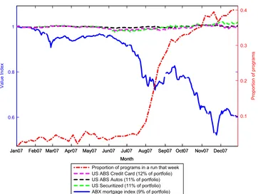
The assumption that runs are triggered by a drop in asset value is strongly supported byFig. 1, which plots price indexes in 2007 for ABCP conduits' main asset classes (solid and dashed lines), and also plots the fraction of ABCP conduits experiencing a run as defined inSection 4.1(dashed-dot line). The figure shows that the ABX index of mortgage-related securities dropped by roughly 20 percentage points in the months before runs intensified.12 Mortgage-related assets
made up 9% of the ABCP industry portfolio in 2007.
We cannot rule out that some of the model's para-meters changed suddenly in mid-2007. However, as we shall see below, the model fits the data remarkably well without these additional assumptions. Moreover, our parameter estimates are forward-looking: we recover the parameter values consistent with yields and run intensi-ties well into the crisis.
Consistent with industry practice, the model assumes that the sponsor extends a line of credit to the conduit during a run. Therefore, the ABCP that matures during a run is replaced by credit-line debt. Since credit-line debt is held by the sponsor, it is not subject to coordination problems. Total debt
Dtin our model is the sum of market-held ABCP and sponsor-held credit-line debt. During a run, the amount of market-held ABCP decreases while sponsor-market-held debt increases. On net, total debtDt increases during a run, because sponsor
debt replaces market debt issued in the past at lower yields. It is unclear whether credit-line debt is senior or junior to ABCP in practice. For tractability, we assume the two types of debt have equal seniority and maturity.13
Note that runs in the model are not caused by idiosyncratic liquidity shocks to creditors. If one individual creditor fails to roll over due to a liquidity shock, another creditor will take up the contract at the break-even yield, preventing a run. In
9At the time of the 2007 crisis, Rule 2a-7 under the Investment
Company Act limited the portfolio share that registered money market mutual funds can invest in eligible securities not rated A-1/P-1 to 5% of the fund portfolio (these securities are typically rated at least A-2/P-2).
10Similar models to ours that incorporate an endogenous default
policy in the spirit of Leland (1998) are Hugonnier, Malamud, and
Morellec (2012),Décamps and Villeneuve (2007), andHe and Milbradt
(2012). These models, however, do not include the possibility of a binding
credit supply constraint, e.g., a credit ratings requirement.
11 A related issue is present inHege and Mella-Barral (2005), in
which creditors dilute each other repeatedly after being offered an alternating sequence of debt renegotiation options. The number of options is finite, so that the last debt renegotiation option is well defined (and given) and the problem can be solved by backward induction.
12The ABX index of mortgage securities is an average across tranches
(from BBB- to AAA) of the ABX.HE indexes for mortgage-backed securities (MBS) originated in the first half of 2006.
13Making credit-line debt junior to ABCP or giving it a longer
maturity than ABCP would make the credit-line debt behave somewhat like an equity stake in the conduit. Incorporating these features into the model would introduce an extra state variable to separately track the
amount of ABCP and credit-line debt. Holding constantr, extending the
maturity of credit-line debt makes total debt increase more slowly during a run, which increases the probability that a conduit recovers from runs, hence reducing investors' willingness to run. That said, sponsors could
require a higherrif their maturity is longer, which could counteract the
Section 4.1we explain how our empirical definition of runs distinguishes lack of rollover for a conduit from a creditor's idiosyncratic withdrawal. Moreover, the data support our assumption that runs on ABCP in 2007 did not result from systemic liquidity shocks to creditors: runs on ABCPpreceded
runs on money market funds, ABCP conduits' main investors. Finally, we assume a conduit never liquidates just a part of its asset to pay running creditors. It is doubtful that conduits would use partial liquidations. The Internet Appendix shows that partial asset sales, far from improving a conduit's health, actually guarantee that the run will continue.14The reason is
that a partial asset sale automatically increases the conduit's leverage. Also, since ABCP assets like trade receivables are very illiquid, it seems plausible that conduits would wait as long as possible before liquidating them.
2.4. Model solution and examples
Appendices A and B contain details on the model's
solution, including a full description of the value function, state variable dynamics, and numerical methods. This subsection describes in nontechnical terms the key fea-tures of the solution.
An infinitesimally small lender knows she will face one of three outcomes, depending on which of the following
events occurs first. The first possible outcome is that the asset matures first, delivering a total payout of minðDt;ytÞ
to lenders as a group. In the second, the loan matures first, allowing the lender to choose between rolling over and running. The third, least desirable outcome is that other lenders run on the conduit, the guarantee fails, and the conduit defaults before the loan matures, which delivers minðDt;αFðytÞÞto the lenders as a group. Therefore, when
choosing whether to roll over, each lender must rationally anticipate other lenders' rollover choices.
As inHe and Xiong (2012a), we solve for the monotone equilibrium in which lenders roll over their debt as long as the state variable does not drop below a threshold. We show that our model's only state variable is inverse leverage (xt), which equals the ratio of the asset's
funda-mental value (yt) to the conduit's total debt (Dt). Applying Ito's Lemma and Eq.(3), it is straightforward to show that inverse leverage follows:
dxt
xt ¼μdtþsdZtþδdt&δRtdt: ð5Þ
In other words, the fraction change in inverse leverage equals the fraction change in the asset's value (μdtþsdZt) plus the
fraction of debt maturing (δdt) minus the fractional amount of new debt issued (δRtdt). In equilibrium, each maturing
creditor compares the conduit's current inverse leveragextto an endogenous, constant threshold,xn, and the creditor runs
as soon asxtoxn.
Jan07 Feb07 Mar07 Apr07 May07 Jun07 Jul07 Aug07 Sep07 Oct07 Nov07 Dec07
0.6 0.8 1
Month
Value Index
Jan07 Feb07 Mar07 Apr07 May07 Jun07 Jul07 Aug07 Sep07 Oct07 Nov07 Dec07 0.1 0.2 0.3 0.4
Month
Proportion of programs
[image:8.595.116.478.69.342.2]Proportion of programs in a run that week US ABS Credit Card (12% of portfolio) US ABS Autos (11% of portfolio) US Securitized (11% of portfolio) ABX mortgage index (9% of portfolio)
Fig. 1. This figure shows the weekly series of prices for several asset categories in the portfolio of ABCP conduits in 2007 (dashed and solid lines), as well as the proportion of ABCP programs experiencing runs in a given week (dashed-dot line). We normalize prices to $1 on January 1, 2007. The ABX index of mortgage securities is an average across tranches (from BBB- to AAA) of the ABX.HE indexes for MBS originated in the first half of 2006. Data for the
remaining asset categories are from Barclays indexes. ‘US Securitized’ is an aggregate of U.S. asset-backed securities, commercial mortgage-backed
securities, and other mortgage-backed securities; this index proxies for the ambiguous‘Securities’category, which makes up 11% of conduit assets in 2007.
Portfolio weights in the legend are from‘The ABC's of ABCP,’an unpublished document from Societe Generale. Data for the proportion of runs are from the
DTCC database on all issues by ABCP programs, where a run is defined as inCovitz, Liang, and Suarez (2013): an ABCP program experiences a run in a given
week if either (1) more than 10% of the program's outstanding paper is scheduled to mature, yet the program does not issue new paper; or (2) the program was in a run the previous week and it does not issue new paper in the current week.
One important implication is that rollover yields depend on leverageðDt=ytÞbut not onytorDtindividually, which is intuitive. More importantly, in equilibrium, creditors will stop rolling over exactly when yield spreads reach the cap,r, since they cannot be compensated for additional default risk. As a consequence, the run thresholdxnwill be the
assets-to-debt ratio where yields first hit their cap. Since sponsors extend the credit line at a below-market spreadr during a run, the sponsors take a loss while supporting the conduit.
Like He and Xiong (2012a), we find that creditors start
running before a conduit becomes insolvent. The reason is that each creditor's rollover decision imposes an externality on the other creditors.
Fig. 2illustrates how leverage and yields adjust over time. The top panel plots the time series of inverse leverage (xt) for
two simulated conduits with the same initial fundamentals but different outcomes. The flat dotted line representsxn, the
predicted run threshold. The dashed line depicts a conduit whose asset's value remains high enough so that the conduit never experiences a run, and all lenders are paid in full. The solid line represents a conduit that experiences two runs when its inverse leverage falls belowxn. During the first run,
the guarantee survives long enough for the conduit to repay all running lenders and begin issuing paper again. The guarantee fails in the second run, causing the conduit to default and liquidate assets, imposing losses on some lenders. The bottom panel of Fig. 2 shows the corresponding rollover yields for those same simulated conduits. Since the conduit represented by the dashed line remains healthy, its yield remains at or near the risk-free rate, ρ¼5%. The yields of the conduit represented by the solid
line spike up and become more volatile as a run becomes
imminent, eventually reaching their cap when the run begins. As soon as this conduit recovers from its first run, yields drop below the cap.
3. Flexible pricing, dilution risk, and the likelihood of runs
Allowing yields to adjust over time significantly changes the likelihood of runs, relative to theHe and Xiong (2012a)
model with constant yields. We compare simulated run probabilities in our model to those inHe and Xiong (2012a, henceforth HX). To make the models comparable, we use the same parameter values where possible, we make the asset's initial market value the same in both models,15 and we
assume conduits in both models initially borrow $1. HX's lenders receive a face value of $1 with a fixed, exogenous yield, so in return for their initial $1 investment, lenders receive debt worth more than $1. Yields in our model are set so that lenders exactly break even, so in return for their initial $1 investment, lenders receive debt worth $1.
0 0.5 1 1.5 2 2.5 3
1.2 1.3 1.4 1.5 1.6 1.7
Time (years)
x=Inverse leverage
0 0.5 1 1.5 2 2.5 3
0.05 0.1 0.15 0.2
Time (years)
r
Annualized yield
=
[image:9.595.124.479.72.355.2]x * = Run threshold
Fig. 2.This figure shows the simulated paths of two conduits with the same initial leverage and parameter values. The top panel shows simulated values of
xt, inverse leverage. The dotted line denotes the run threshold. The bottom panel shows simulated paths of annual yields at rollover for the same two
conduits. The risk-free rate is 5% and the cap on the rollover yield is 20%.
15The asset pays interim cash flows at raterinHe and Xiong (2012a),
but our model has no interim cash flows. Setting the asset's value equal in
the two models requires choosing initial fundamentaly0by solving
FHX yHX o ! "
¼F y! "0
)ρr
þϕþy
HX
0 ϕ ρþϕ&μ¼y0
ϕ ρþϕ&μ;
wherey0 (y0
HX
) is the asset's initial fundamental value in our (HX's)
model. In the first analysis we setyHX
0 ¼2:1. In the second analysis we set
yHX
We compare the two models inTable 1. We show results using HX's calibrated parameter values (left-hand columns) and our estimated parameter values (right-hand columns). We repeat the analysis using several values ofr (our model's cap on yield spreads) and HX's exogenous yield.16
Panel A shows that runs are 1.31–51 times more likely
in our model than in HX's when we use HX's calibrated parameter values. Runs are especially more likely in our model if HX's exogenous yield is higher, because HX's investors are less willing to run on debt that offers a higher interest rate. Runs are not always more likely in our model, however. With estimated parameter values, we see that when HX's fixed yield is sufficiently low, our model produces 35% fewer runs than HX's model.
Intuitively, flexible yields influence runs through three channels. The first two channels make runs less likely in our model compared to HX. First, conduits in our model can initially borrow at low interest rates, allowing them to start with lower leverage (Panel C inTable 1). Second, being able to raise yields in bad times helps convince lenders to roll over.
This relative advantage is especially large when HX's fixed yield is very low, which explains why our model produces fewer runs than HX only when HX's fixed yield is very low (e.g., ten basis points (b.p.) above the risk-free rate inTable 1). The third channel makes runs more likely in our model and typically outweighs the previous two channels. Flexible yields introduce a new risk, which we call‘dilution risk,’on
top of rollover risk and insolvency risk. If conditions deterio-rate for a conduit, it will have to offer higher yields to induce rollover. These higher yields increase the conduit's debt by more, which dilutes earlier lenders' stakes. This effect depends strongly on the assumption that bankruptcy proceeds are distributed pro rata, consistent with ABCP industry practice. A lender deciding whether to roll over in our model antici-pates the possibility of being diluted in the future if conditions worsen. The lender therefore preemptively demands a higher yield to compensate her for dilution risk. Since dilution risk increases yields for any given level of leverage, yields hit their cap at lower leverage, implying a higher run threshold for inverse leverage,xn. Panel B in Table 1shows that the run
threshold is indeed higher in our model compared to HX, which tends to make runs more likely.
4. Estimation
[image:10.595.48.546.176.424.2]This section describes the data, SMM estimator, and intuition behind the estimation method.
Table 1
The effect of flexible yields on runs.
This table compares the predictions from our model to the predictions ofHe and Xiong (2012a), denoted HX. Yields change over time in our model,
whereas yields are constant in HX. The columns on the left use HX's calibrated values:ρ¼1:5%,ϕ¼0.077,α¼55%,s¼20%,μ¼1:5%,y0¼1.4,δ¼10, and
θ¼5. The columns on the right use estimated parameter values for the weak-guarantee subsample inTable 4. Panel A shows the fraction of simulated
conduits that experience a run in our model within one year, divided by the corresponding fraction from HX. Panel B shows the run threshold in our model
(xn) divided by the run threshold in HX. Panel C shows the conduit's initial inverse leverage in our model (x
0) divided by the conduit's initial inverse
leverage in HX; these results are identical out to two digits for the three values ofr. The parameterris our model's cap on yield spreads, andρis the
risk-free rate, sorþρis the capped rollover yield.
Panel A: Ratio of the one-year run probability in our model to that in HX
Using HX parameters Using estimated parameters
HX's fixed yield: 5% 7% 9% ρþ0:1% ρþ0:3% ρþ0:5%
rþρ¼15% 1.31 3.73 50.64 0.65 1.48 3.61
rþρ¼20% 1.29 3.64 49.08
rþρ¼25% 1.28 3.56 47.65
Panel B: Ratio of the run threshold in our model to that in HX
Using HX parameters Using estimated parameters
HX's fixed yield: 5% 7% 9% ρþ0:1% ρþ0:3% ρþ0:5%
rþρ¼15% 1.43 1.77 2.29 1.22 1.24 1.26
rþρ¼20% 1.42 1.75 2.28
rþρ¼25% 1.41 1.74 2.26
Panel C: Ratio of initial inverse leverage in our model to that in HX
Using HX parameters Using estimated parameters
HX's fixed yield: 5% 7% 9% ρþ0:1% ρþ0:3% ρþ0:5%
1.38 1.54 1.70 1.25 1.26 1.27
16In the first analysis, HX's fixed yield is centered at its calibrated
value, 7%. We choose values of r much higher than HX's fixed yield,
because higher values ofr make runs less likely in our model, all else
equal. We find that despite these highrvalues, runs are still more likely
in our model than in HX. In the right-hand columns,ris at its estimated
4.1. Data
The dataset used in this paper includes all issuance transactions in the U.S. ABCP market from the Depository Trust and Clearing Corporation (DTCC). The data contain the outstanding amount of paper for a conduit each week and the distribution of maturities and yields each day a conduit issues ABCP.
We obtain data on each conduit's guarantee type from Moody's Investors Service. ABCP conduits are structured with one of four possible types of guarantees (Acharya, Schnabl, and Suarez, 2013). In conduits structured with a full credit guarantee, the sponsor provides a line that can be drawn regardless of asset defaults. In conduits with a full liquidity guarantee, the sponsor provides a line that can be drawn as long as the assets are not in default. In SIV guarantees, only a portion of conduit liabilities are covered by the line. In conduits created to issue extendible notes, issuers have the option of extending the maturity of the paper at a prespecified penalty rate, exposing investors to asset defaults during the extension period. From the point of view of investors, full credit and full liquidity guarantees offer relatively stronger protection.
Covitz, Liang, and Suarez (2013)show that conduits with stronger guarantees experienced significantly fewer runs in 2007. For this reason, we estimate the model in two sub-samples based on guarantee strength.17The‘strong-guarantee’
subsample contains the 191 conduits with either a full credit or full liquidity guarantee; 45% of these conduits experienced a run in 2007. The‘weak-guarantee’subsample contains the 90 conduits with either an SIV guarantee or extendible paper; 83% of these conduits experienced a run in 2007. As in many structural estimation papers (e.g., Hennessy and Whited,
2007;Strebulaev and Whited, 2012), we assume parameter
values are constant within each subsample. Our parameter estimates therefore characterize an average conduit within each subsample.
We use the method ofCovitz, Liang, and Suarez (2013)
to identify runs in the data. More specifically, we say that conduitiis in a run in weektif either (1) more than 10% of the conduit's outstanding paper is scheduled to mature, yet the conduit does not issue new paper; or (2) the conduit was in a run in weekt&1 and the conduit does not
issue new paper in weekt. We say that a conduit recovers from a run in weektif it issues paper that week but was in a run the previous week. By using the total amount a conduit rolls over, this definition avoids misclassifying as runs situations in which one creditor replaces another due to the first creditor's idiosyncratic liquidity needs.
We measure each conduit's rollover spread as the dollar-weighted average annualized yield for paper issued on Thursday of weekt, minus the prevailing federal funds rate.18If the conduit did not issue paper on Thursday, we
move one day ahead until finding an issuance transaction in weekt.
The total amount of ABCP outstanding peaked at $1.2 trillion in late July 2007. At that time, 339 ABCP conduits operated. Yield spreads averaged five b.p. in the first half of the year. In August 2007, the amount of debt outstanding plunged by $190 billion and average spreads increased to 74 b.p.19Roughly 25% of ABCP conduits experienced a run
in August, according to our measure. Rollover yields remained high and volatile in the second half of 2007. By the end of the year, the total amount of ABCP out-standing was 30% below its peak.
Our analysis uses all transactions from 2007. We face the trade-off that a larger sample would provide more precise estimates, but it would be harder to argue that model parameters are constant over a longer period. Year 2007 is an ideal sample because it contains many runs and also several months of pre-run data. Adding observations from 2006 would not improve precision, because yield spreads were near zero and there were no runs. Adding observations from 2008 would potentially contaminate results with effects from the Lehman Brothers failure and subsequent government interventions.
4.2. Estimator
First we explain how we measure parameters ρ, δ, ϕ, and μdirectly from the data. Next we describe the SMM estimation of the four remaining parameters.
Investors' discount rateρis also the risk-free interest rate. We setρto 4.9%, the annualized yield of one-month T-bills at the beginning of 2007.
The average debt maturity in our model is 1/δ. We set 1/δto 0.101 years (37 days), the average maturity of ABCP as of March 2007. We use the same value of 1/δ in both subsamples because there is no significant difference in maturities between them in early 2007, and, as we show later, such small differences in maturity have a very small effect on run probabilities. The assumption that δ is constant over time could be somewhat problematic given that most conduits experienced a rat-race whereby they offered shorter maturities to prevent creditors from run-ning (Brunnermeier and Oehmke, 2013). While average rollover maturities do decrease in the six months preced-ing runs in our data, we find that they only drop from 38 days to 27 days. By contrast, changes in ABCP rollover yields were more dramatic, which is why we focus on time-varying yields in this paper. Extending the model to include endogenous maturity is an interesting avenue for future work.
The expected conduit life span, which corresponds to the asset's duration, is 1=ϕ. Adding the assumption that new ABCP conduits are created at a constant rate, the model predicts that the average age of conduits alive at any snapshot in time equals 1=ϕ. The average age of ABCP
17Ideally, we would estimate the model in even finer-grained
subsamples, but the small number of conduits prevents us from doing so.
18We choose Thursday because amounts outstanding are measured
at the end of Wednesday each week.
19Important events in early August 2007 include American Home
conduits operating in July 2007 is 5.8 years, so we set ϕ to 1/5.8.
The parameter μ, which represents the asset's growth rate, is not identified from our data. The parameterμis not the asset's expected return, which equals ρ (investors' discount rate). Therefore,μwould not be identified directly from average returns on ABCP assets, even if we had those data. The asset's return at τϕ, the instant it matures, is
positive (negative) ifμis less than (greater than)ρ.20These
event returns could help us identifyμ, but unfortunately, those data are not available either. For our main results we setμ¼ρ, which assumes it is neither good nor bad news for investors when the asset matures. For robustness, in the Internet Appendix we show that parameter estimates do not change significantly if we setμtoρþ1%per year.
We do not estimate conduits' initial leverage, 1=x0. Leverage at the beginning of our sample is not well identified, since yield spreads in the first half of 2007 were near zero. When yield spreads are near zero, the model's mapping from conduit leverage to yields is almost flat. Intuitively, since spreads were near zero at the beginning of 2007, we know leverage was low at that time, but we do not know how low.
Fortunately, we do not need to know 1=x0 to estimate the model, because the moments we use in SMM estima-tion are independent of its value. Some of our moments are conditional on a run starting, at which point xt has reachedxn. Since the predictedxndoes not depend onx
0,
then neither do these moments. The remaining moments (both simulated and actual) are forward-looking and only use conduit/week observations where yield spreads are at least ten b.p. per year. At spreads of ten b.p. and above, the mapping between leverage and spreads is no longer flat. Therefore, the ten b.p. threshold forces us to only use observations that exceed a certain leverage threshold. Once we condition on leverage being above this threshold, the forward-looking moments no longer depend on initial leverage, 1=x0, because leverage is the model's only state variable. Our simulated conduits start with 1=x0 low enough that their initial spreads are well below ten b.p., as they were in early 2007. We simulate a large enough sample so that we have many observations with spreads above ten b.p., which allows us to measure our simulated moments precisely.
The remaining parameters to estimate are s (asset volatility),θ(the weakness of guarantees),α(asset liquid-ity), andr (the cap on yield spreads). We estimatesas a structural parameter instead of using price data on ABCP assets, because those data are not available. Data on conduit-level asset holdings are not publicly available. Even constructing an industry-wide price index is impos-sible, because we lack price data for illiquid assets like trade receivables, the largest ABCP asset class.
We estimate the four remaining parameters using the simulated method of moments (SMM). This estimator chooses parameter values that minimize the distance between moments generated by the model and their sample analogs.
The following subsection defines our 13 moments and explains how they identify our parameters. Additional details are inAppendix C.
4.3. Identification and choice of moments
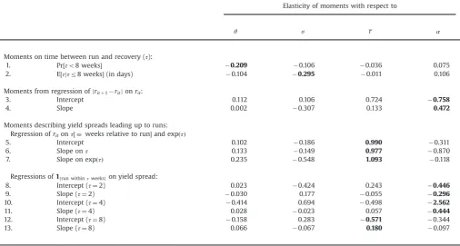
Since we conduct a structural estimation, identification requires choosing moments whose predicted values move in different ways with the model's parameters, and choos-ing enough moments so there is a unique parameter vector that makes the model fit the data as closely as possible. This subsection explains how our 13 moments vary with the four parameters. Each moment depends on all model parameters, often through the parameters' effect on lever-age dynamics or the run threshold. Below, we emphasize which parameters matter most for each moment, which explains which features of the data are most important for each parameter. To illustrate,Table 2presents the Jacobian matrix containing the derivatives of our 13 moments with respect to our four parameters.21For both subsamples, the
Jacobians have full rank and a low condition number,22
which confirms local identification.
4.3.1. Recoveries from runs
The first moment is the fraction of runs that are followed by a recovery, meaning that the conduit issues paper again, at least once within eight weeks of the run's start.23 In our model, once a run starts, the probability
of a recovery decreases in θ, the guarantee's weakness. Intuitively, a strong guarantee buys time for asset values to improve so the conduit can exit the run. The Jacobian in
Table 2confirms that this first moment is most sensitive to θand fairly insensitive to other parameters.
The second moment is the average number of days until recovery for those runs that experience a recovery within eight weeks of the run's start. Conditional on a recovery within a given period, the expected time to recover is shorter for higher asset volatilitys, because higher volatility makes the conduit re-cross the run threshold sooner.Table 2shows that this moment is indeed most sensitive tos.
The remaining parameters have an indirect effect on our first two moments through the run threshold, xn.
In this case, however, these effects are relatively small, confirming that the recovery probability and the expected recovery time essentially identifysandθonly.
4.3.2. Yield volatility
The moments we use to summarize yield spread volatility are the coefficientsβ0andβ1from the following
20The asset's value immediately prior toτ
ϕisFðyτϕÞ. The asset's value
immediately after isyτϕ.
21We present the Jacobian evaluated at estimated parameter values
for the weak-guarantee subsample. The properties of the Jacobian for the strong-guarantee subsample are very similar. In the interest of space, we report the Jacobian for the strong-guarantee subsample only in the Internet Appendix. To make the sensitivities comparable across
moments, we express them as elasticities, e.g.,ð∂mi=∂αÞ ) ðα=miÞis the
elasticity of thei-th moment toα.
22The condition number of a matrix is the ratio of its largest to
smallest singular value. Large condition numbers indicate a nearly singular matrix.
23We find empirically that if a run is not followed by a recovery
panel regression of absolute changes in yield spreads on the lagged yield spread24:
jrit&rit&1j¼β0þβ1rit&1þɛit: ð6Þ The predicted yield spread volatility is given by
vartðdrtÞ ¼ xt∂r
∂x xt;x
n
! " % &2
s2dt: ð7Þ
The first term in(7)increases in the yield spread, so the model predicts that yield volatility is high when yield spreads are high. In other words, we should findβ140 in
(6). The model therefore produces time-varying volatility in debt yields, even though asset volatility,s, is constant. The term ∂r=∂x in (7) goes to zero as yield spreads approach zero. Intuitively, if a conduit's leverage is extre-mely low, yield spreads are near zero, and small changes in leverage still keep spreads near zero. Therefore, the model imposes β0*0 as an overidentifying moment condition, regardless of parameter values. As a result, yield volatility
is informative about asset volatility only when spreads are high.
Asset volatility has a direct, positive effect on yield volatility through the s term in (7), and also a negative effect via the first term: a highersdecreases the absolute slopej∂r=∂xjfor givenr, providedris high enough. For our parameter estimates, and given that we measure our moments conditional on spreads exceeding ten b.p., the second effect dominates: we find that the sensitivity of yield volatility to yield levelsdecreases with asset volati-lity, sosis partially identified off its negative effect onβ1. Indeed,Table 2confirms thatβ1depends negatively ons. Note too thatαhas a strong positive effect onβ1. The reason is that an increase in asset liquidity decreases the run threshold,xn, which in turn implies a higher absolute
slope j∂r=∂xj for any given r. Intuitively, if two conduits with assets of different liquidity have reached the same yield spreads, it must be that yields are increasing faster for the one with higher liquidity.
4.3.3. Yield spreads preceding runs
[image:13.595.47.554.197.468.2]Our next three moments measure average yield spreads in event time before runs. We defineτitas the number of weeks relative to the run's start, and we use the subset of data from the 12 weeks preceding each run to estimate the
Table 2
Estimated Jacobian matrix.
This table presents the estimates of the Jacobian matrix for the 13 moment conditions in our SMM estimation procedure, for the subsample of 90 ABCP conduits in 2007 with SIV or extendible credit guarantees. Moment 1 is the probability that a conduit experiences a recovery within eight weeks of a run's start. Moment 2 is the average number of days between the run's start and recovery, conditional on a recovery occurring within eight weeks of the run's
start. Moments 3 and 4 are the intercept and slope from a regression of absolute changes in yield spreads on the lagged yield spread. Moments 5–7 are the
intercept and slopes from a regression of yield spreads on the number of weeks relative to a run and the exponent of that same number. Moments 8–13
come from three regressions, each of the indicator1frun withinτweeksgon the current yield spread. The three regressions useτ¼2, 4, and 8 weeks. Each row of
each matrix contains the estimated elasticities of the given moment with respect to the parameters across its columns. Parameters are estimated by SMM,
which chooses values that minimize the distance between actual and simulated moments.Section 2describes the model used to simulate moments. The
number highlighted in each row in bold type face corresponds to the moment's highest elasticity in absolute value.
Elasticity of moments with respect to
θ s r α
Moments on time between run and recovery (τ):
1. Pr½τo8 weeks( &0.209 &0.106 &0.036 0.075
2. E½τjτr8 weeks((in days) &0.104 &0.295 &0.011 0.106
Moments from regression ofjritþ1&ritjonrit:
3. Intercept 0.112 0.106 0.724 &0.758
4. Slope 0.002 &0.307 0.133 0.472
Moments describing yield spreads leading up to runs:
Regression ofritonτ½ %weeks relative to run(and expðτÞ
5. Intercept 0.102 &0.186 0.990 &0.311
6. Slope onτ 0.133 &0.149 0.977 &0.870
7. Slope on expðτÞ 0.235 &0.548 1.093 &0.118
Regressions of1frun withinτweeksgon yield spread:
8. Intercept (τ¼2) 0.023 &0.424 0.243 &0.446
9. Slope (τ¼2) &0.030 0.177 &0.055 &0.296
10. Intercept (τ¼4) &0.414 0.694 &0.498 &2.562
11. Slope (τ¼4) 0.028 &0.023 0.057 &0.444
12. Intercept (τ¼8) &0.158 0.283 &0.571 &0.344
13. Slope (τ¼8) 0.066 &0.067 0.180 &0.097
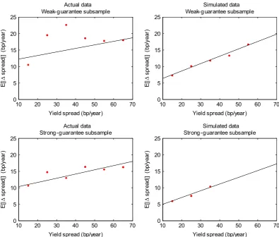
24 Fig. 3plots the nonparametric relation in the data and shows that
the linear, parametric specification in Eq.(6)fits the data quite well. We
discard observations with ritr10 basis points per year so that this
regression
rit¼γ0þγ1τitþγ2expðτitÞþɛit: ð8Þ
Fig. 4shows that this specification fits the path of average yield spreads leading up to runs fairly well. Our next three moments are the coefficientsγ0,γ1, andγ2, which summar-ize event-time spreads.
As discussed inSection 2.4, the model predicts that a run begins the instant yield spreads hit r. Since we only have weekly data, we cannot directly observe yields spreads the instant a run begins. However, yield spreads in the weeks leading up to runs are informative about the yield spread the instant a run begins. Specifically, the level (γ0), slope (γ1), and curvature (γ2) of the event-time plot of average spreads before runs all increase in r. The moments γ0, γ1, andγ2therefore help identifyr. Consistent with this reasoning, the estimated Jacobian shows that these three moments are by far most sensitive torand therefore effectively identify this parameter.
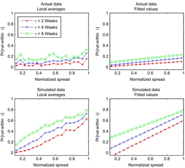
4.3.4. Run probabilities
Our next moments are from three regressions that fore-cast future runs using current yield spreads. The regressions
have the form25
1frun withinτweeks of ritg¼λ0τþλ1τmaxrrit
iþɛit; ð9Þ
where maxri proxies for conduit i's maximum yield spread, r. Since runs in the model begin as soon as rit hitsr, the higher the fractionrit=r, the closer the conduit is
to a run.26For a conduit that experiences a run, the most
natural proxy for r is the conduit's maximum observed yield spread. For conduits that never experience a run or
10 20 30 40 50 60 70
0 5 10 15 20 25
Yield spread (bp/year)
|[
E
∆
)r
ae
y/p
b(
]|d
aer
ps
Actual data Weak-guarantee subsample
10 20 30 40 50 60 70
0 5 10 15 20 25
Yield spread (bp/year)
|[
E
∆
)r
ae
y/p
b(
]|d
aer
ps
Simulated data Weak-guarantee subsample
10 20 30 40 50 60 70
0 5 10 15 20 25
Yield spread (bp/year)
|[
E
∆
)r
ae
y/p
b(
]|d
aer
ps
Actual data Strong-guarantee subsample
10 20 30 40 50 60 70
0 5 10 15 20 25
Yield spread (bp/year)
|[
E
∆
)r
ae
y/p
b(
]|d
aer
ps
[image:14.595.97.493.74.410.2]Simulated data Strong-guarantee subsample
Fig. 3. This figure shows the relation between yield spread volatility and the yield spread level, both measured in basis points per year (bp/year). The vertical axis is the absolute value of one-week changes in yield spread. The horizontal axis is the lagged yield spread. The left-hand (right-hand) panels show results in actual (simulated) data. The top panels show results for the weak-guarantee subsample, which contains the 90 ABCP conduits in 2007 with extendible or SIV guarantees. The bottom panels show results for the strong-guarantee subsample, which contains the 191 ABCP conduits in 2007 with full credit or full liquidity credit guarantees. The points show local averages, and the solid line shows predicted values from a regression of absolute changes in yield spreads on the lagged yield spread. The intercept and slope from this regression provide two of the 13 moments used in the SMM estimation. The reason there are fewer points in the bottom-right panel compared to the bottom-left panel is that the estimated cap on yield spread is 36 basis points in the
strong-guarantee subsample; all simulated spreads are thereforer36 basis points, whereas there are a few spreads436 basis points in the actual data.
25Following Angrist and Pischke (2009), we use ordinary least
squares (OLS) rather than a probit/logit model, because OLS slopes are easier to interpret, and OLS provides the closest linear approximation of
the conditional expectation function.Figs. 5and6show that the linear
specification in(9)fits the raw data quite well. As in regression(6), we
exclude observations withrito10 basis points per year; run probabilities
for these observations are sensitive to the choice of initial conditionx0in
our simulations, and we want moments that do not depend onx0.
26Empirically, we find some heterogeneity in maxr
i. Since the
estimation procedure assumesr is constant across conduits, our
esti-mated r reflects the yield-spread cap for the average conduit. We
high yield spreads, we use information from those that do experience runs: we setmaxrito the larger of the conduit's maximum observed yield spread (since the conduit'sris at least this large) and the averagemaxracross conduits that did experience runs (a proxy for the average r in the sample). We estimate regression (9) for forecasting hor-izons ofτ¼2;4, and 8 weeks. Our last six moments are the
coefficientsλ0τ andλ1τfrom those three regressions.
The momentλ0τsummarizes the run probability when
spreads are near zero. Therefore, this moment depends negatively on the distance betweenx0and the run thresh-old,xn, which is itself decreasing inα.Table 2shows that λ0τ is strongly decreasing in α, so these moments
effec-tively identify α through α's effect on the run threshold. Note that a higherr also implies a lower run probability when yield spreads are near zero. However, sinceαhas a strong effect on yield levels, which impact the drift of leverage, a lowerαnot only implies a lower distance to the run threshold, but also a quicker transition to it. As a consequence, the difference between a conduit that never experiences a run as opposed to a conduit that experiences a runquicklyis more likely to be due to a difference inα rather than r. Consistent with the above intuition, the
estimated Jacobian shows that λ0τ is more sensitive to α,
than r for the two- and four-week run probabilities, but not for the eight-week probabilities.
5. Estimation results
We start by assessing how well our model lines up with data from the 2007 ABCP crisis. We then present and interpret the structural parameter estimates.
5.1. Model fit
5.1.1. Moments used in SMM estimation
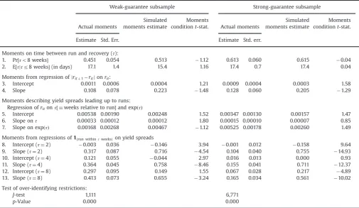
Table 3compares actual and simulated values of our 13
moments. The left (right) half of the table shows moments in the weak- (strong-) guarantee subsample.
Moments 1 and 2 focus on recoveries from runs. Comparing moment one across subsamples, we see that the probability of a recovery is significantly higher (t¼2.0)
in the strong-guarantee subsample, consistent with the model's prediction. When recoveries do occur, they arrive 17 days after the run's start, on average (moment 2). Comparing simulated and actual moments, the model
-25 -20 -15 -10 -5 0
0 10 20 30 40 50 60 70
Actual data Weak-guarantee subsample
)r
ae
y/p
b(
da
er
ps
dlei
Y
Weeks relative to run
-25 -20 -15 -10 -5 0
0 10 20 30 40 50 60 70
Simulated data Weak-guarantee subsample
)r
ae
y/p
b(
da
er
ps
dlei
Y
Weeks relative to run
-25 -20 -15 -10 -5 0
0 10 20 30 40 50 60 70
Actual data Strong-guarantee subsample
)r
ae
y/p
b(
da
er
ps
dlei
Y
Weeks relative to run
-25 -20 -15 -10 -5 0
0 10 20 30 40 50 60 70
Simulated data Strong-guarantee subsample
)r
ae
y/p
b(
da
er
ps
dlei
Y
[image:15.595.99.500.75.414.2]Weeks relative to run
Fig. 4.This figure plots average yield spreads (basis points per year, bp/year) in event time leading up to runs in event week zero. The left-hand (right-hand) panels show results in actual (simulated) data. The top panels show results for the weak-guarantee subsample, which contains the 90 ABCP conduits in 2007 with extendible or SIV guarantees. The bottom panels show results for the strong-guarantee subsample, which contains the 191 ABCP conduits in 2007 with full credit or full liquidity credit guarantees. The points show the average yield spread in each week. The solid line shows the predicted values from the regression of yield spreads on the number of weeks relative to the run and the exponent of that same number. The intercept and
two slopes from this regression provide three of the 13 moments used in SMM estimation. The solid line starts at week&12 because the regression only