A hybrid method for modelling two dimensional non-breaking and breaking waves

City, University of London Institutional Repository

Citation:

This is the accepted version of the paper.

This version of the publication may differ from the final published

version.

Permanent repository link:

Link to published version:

Copyright and reuse: City Research Online aims to make research

outputs of City, University of London available to a wider audience.

Copyright and Moral Rights remain with the author(s) and/or copyright

holders. URLs from City Research Online may be freely distributed and

linked to.

City Research Online: http://openaccess.city.ac.uk/ [email protected]

A Hybrid Method for Modelling Two Dimensional Non-breaking

and Breaking Waves

V.Sriram1,2 , Q.W. Ma2 and T.Schlurmann3

1 _{Department of Ocean Engineering, IIT Madras, India}

2 _{School of Engineering and Mathematical Sciences, City University London, United Kingdom}

3_{Franzius Institute, Leibniz University of Hannover, Germany}

Abstract

This is the first paper to present a hybrid method coupling a Improved Meshless Local Petrov Galerkin method with Rankine source solution (IMLPG_R) based on the Navier Stokes (NS) equations, with a finite element method (FEM) based on the fully nonlinear potential flow theory (FNPT) in order to efficiently simulate the violent waves and their interaction with marine structures. The two models are strongly coupled in space and time domains using a moving overlapping zone, wherein the information from both the solvers is exchanged. In the time domain, the Runge-Kutta 2nd order method is nested with a predictor-corrector scheme. In the space domain, numerical techniques including ‘Feeding Particles’ and two-layer particle interpolation with relaxation coefficients are introduced to achieve the robust coupling of the two models. The properties and behaviours of the new hybrid model are tested by modelling a regular wave, solitary wave and Cnoidal wave including breaking and overtopping. It is validated by comparing the results of the method with analytical solutions, results from other methods and experimental data. The paper demonstrates that the method can produce satisfactory results but uses much less computational time compared with a method based on the full NS model.

Keywords: FNPT, Navier-Stokes, FEM, IMLPG_R, Hybrid methods, breaking and non breaking waves, Cnoidal, Solitary waves.

1. Introduction

The available numerical models for strongly nonlinear interactions between water waves and marine structures are mainly based on solving either the fully nonlinear potential flow theory (FNPT) or the Navier Stokes (NS) equations. The problems formulated by the FNPT model are usually solved by a time marching procedure, originally proposed by Longuet – Higgins and Cokelet [1]. In this procedure, the key task is to solve the boundary value problem (BVP) for the velocity potential at each time step by using a numerical method, such as the boundary element method (BEM) and the finite element method (FEM). The BEM including higher order BEM and those based on domain decomposition technique has been attempted by many researchers, as reviewed by Kim et al. [2]. The FEM was used by Wu and Eatock Taylor [3] for the 2D cases and by Ma et al. [4] for 3D cases, and it was further extended to handle complex objects and floating bodies simulations forming the QALE-FEM (Quasi-Arbitrary Lagrangian and Eulerian

*Manuscript

finite element method) by Ma et al [5,6], Yan et al [7,8,9] and SALE-FEM (Semi-Arbitrary Lagrangian and Eulerian finite element method) by Sriram [10], respectively. It has been shown that the FEM is more efficient for modelling strongly nonlinear waves while the BEM is more efficient for modelling linear or weak nonlinear problems [9]. The problems formulated by using the NS model are usually solved by employing a mesh-based method or a meshfree method. There are a large number of publications for both approaches. Extensive review on them would diverse the focus of this paper but a brief review will be given here for completeness. In the mesh based methods, finite volume methods [11-14] and finite difference methods [18-19] have been extensively used. In order to handle large domains, a multi-resolution capability and far-field boundary conditions to the regular fixed-grid NS solver have also been proposed using chimera and moving grid methods [15-17]. The advantage of such a strategy is the use of regular grids that could avoid the numerical stability issues; however, if viscous effects are introduced then there will be a restriction on the length time step. On the other hand, the meshfree (or particle) methods have been recognised as promising approaches in recent years, particularly for modelling violent waves and their interaction with structures owing to their advantages that meshes are not required and numerical diffusion associated with convection terms is eliminated compared to traditional mesh based methods. The notable papers based on particle methods for the topics related to wave-structure interactions include but are not limited to references [22-24] for using smoothed particle hydrodynamics (SPH), [25] for using moving particle semi-implicit method (MPS), [26-27] for using Meshless Local Petrov Galerkin with Rankine Source (MLPG_R). Some simplified test cases reported in the literature using these models showed a good agreement with the experimental measurements, see for example, [1-10,28] for the FNPT models and [22-25, 29-31] for the NS models.

These two types of models have their own advantages and disadvantages. When using the FNPT models, one cannot model breaking waves or consider viscous effects, but can conserve the energy for long time and long distance simulations with higher computational efficiency. Whereas, when employing the NS models, one could handle violent waves and consider viscous effects but normally see loss of energy for long time and long distance simulation and use prohibited computational time. Due to their disadvantages, neither of the two types of models is suitable for modelling large scale wave propagation incorporating both non-breaking and breaking processes, such as the wave scenarios in a large area from offshore to coastal zone. The ideal model should meet the following criteria:

i) To properly resolve the physical scales of interest in wave-structure

interactions and

ii) The simulations must be sufficiently accurate and efficient for practical applications.

Hybrid models seem to be a promising one that can meet the criteria. In such a model, one may use the nonlinear potential flow theory (FNPT) and full NS equations in sub-domains wherever appropriate, thus not compromising on the physics.

The idea of the hybrid model has been reported in recent literature. The classification of

literature is broadly classified into weak and strong couplings of two models. In the weak coupling, initially only one solver will be run completely without the need for other, the

result is then feed into other solver to complete the simulation. Whereas, in the strong

coupling the information from both the models are exchanged, and their solutions are

mutually dependent. Notable works on weak coupling were presented by Lachaume et al.

[33] and Biausser et al. [37]. In the references, the FNPT model based on the BEM was combined with the NS model based on a finite volume method (FVM) for the simulation of solitary wave breaking over the sloped terrain. Yan and Ma [55] and Hildebrant et al.

[54] used the weak coupling between the FNPT model based on finite element method

and commercial software STAR-CCM and ANSYS, respectively. Janssen et al. [39] coupled the BEM based on the FNPT with the discrete Boltzmann equation using Lattice Boltzmann method to study the solitary wave breaking. The strong coupling can be further classified into explicit, implicit and intrinsic technique.In explicit coupling, the FNPT solver results are obtained using the information from the previous time step and the results are then feed into the NS solver to complete the simulation at every time step. In implicit coupling, every time step is split into several sub-steps. In the sub-steps, the results from the FNPT solver are not only sent to the NS solver, the results from the NS

solver are also feed back to the FNPT solver. Whereas, in the intrinsic technique both

solvers are iterated till convergence is reached. So far no papers using the intrinsic

technique have been found, perhaps because of its high computational cost. On the strong coupling approach, the notable works were carried out by Grilli [34], Kim et al [35], Guo et al [36] by combining the FNPT model based on the BEM with the NS model based on the FVM. Colicchio et al. [38] adopted a similar method to model a dam breaking problem and applied it to wave slamming on the deck. The two models are strongly coupled through a fixed overlapping zone. Fujima et al. [32] developed a hybrid model for numerically simulating tsunami around structures. In their work, the nonlinear long wave (or shallow water) equations are used to model the exterior domain, whereas the NS model with k-İ turbulence is employed to model the inner three-dimensional (3D) domain. Further, comparison with the laboratory experiment showed that their hybrid model was able to reproduce the 3D characteristics of flow around structure, and comparison with similar simulation using a full 3D NS model proved that the hybrid model could reduce the computational time significantly. Sitanggang [40] developed a hybrid coupling between the Boussinesq model and the NS model based on a finite difference method (FDM), again fixed overlapping zone was used to transfer the information between the two models. In coupling mesh-based methods with meshless methods, Sueyoshi et al. [41] used the BEM and the MPS for developing a two-way coupled algorithm, modelling the top part of the domain near the free surface using the MPS method and the bottom part of the domain using the BEM. The information between the two solvers were transferred through a fixed boundary interface. Narayanaswamy et al. [42] and Kassiotis et al. [43] used the weak coupling of the Boussinesq model with the SPH method for solitary wave simulations without feedback from the SPH method to the Boussinesq model, a fixed overlapping zone was employed to transfer the information from the Boussinesq model to the SPH method.

violent wave problems, which has not been attempted before. The main idea of this method is that the FNPT-based finite element method is employed in the region where waves are not breaking while the NS-based IMLPG_R method is adopted in the region where breaking/broken waves are involved. They are nearly fully coupled in the sense that the IMLPG_R method does not only receive the information from the FNPT-based finite element method but also provides information back to the other solver. The new hybrid method will be shortened as FEM-MLPG_R in this paper.

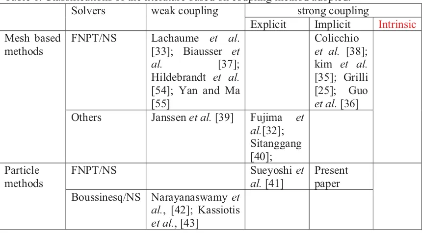
Table 1. Classifications of the literature based on coupling method adopted.

Solvers weak coupling strong coupling

Explicit Implicit Intrinsic

Mesh based methods

FNPT/NS Lachaume et al.

[33]; Biausser et

al. [37];

Hildebrandt et al.

[54]; Yan and Ma [55]

Colicchio

et al. [38];

kim et al.

[35]; Grilli [25]; Guo

et al. [36]

Others Janssen et al. [39] Fujima et

al.[32]; Sitanggang [40]; Particle

methods

FNPT/NS Sueyoshi et

al. [41]

Present paper Boussinesq/NS Narayanaswamy et

al., [42]; Kassiotis

et al., [43]

This method, compared with other hybrid methods listed above, has the distinctive features. (1) The FNPT-based finite element method can model any steep waves in water from deep to shallow. (2) The FEM can be more than 10 times faster than the BEM for modelling large scale fully nonlinear waves [7, 9]. (3) The FEM can provide solution at any points in the flow field, while the direct solution of the BEM is only given on boundaries. This makes the FEM more advantageous over the BEM if coupled with the methods based on the NS model that always needs the information in whole flow field, not only on boundaries. (4) The IMLPG_R method [27,31] is based on a weak form of the Poisson’s equation. In the weak form, there are only unknown functions without any derivatives. Therefore, there is no need to numerically approximate the derivatives that potentially lead to larger error or more numerical diffusion compared with numerical approximation of functions. Due to this feature, the IMLPG_R method is potentially more accurate than other meshless methods, like the incompressible SPH [22] and MPS [25], based on the Poisson’s equation, which numerically approximate the second order derivatives directly. Our previous work [27,31,44-46] has demonstrated the advantages of the IMLPG_R method.

coupling them will be detailed, in which the concept and technique of moving overlapping zone will be introduced. The various properties of the new model will be tested for small waves with analytical solution, and for solitary waves with the experimental data from literatures, and for Cnoidal waves using the experimental measurement reported in the author’s published papers. The attention is particularly focused on influence of the width and position of the overlapping zone with the error analysis. Finally, the paper ends with the typical application of the model to breaking wave overtopping and solitary waves over a slope, and with discussion about computational efficiency.

2.0 Formulation of the Problem

2.1. Mathematical Formulation

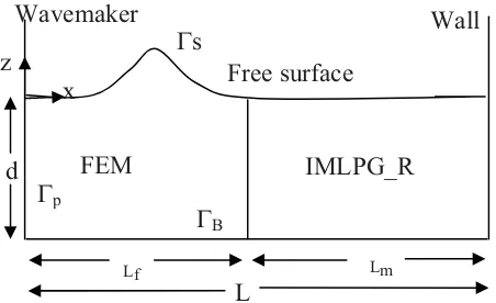
The two dimensional fluid motion is defined with respect to the fixed Cartesian coordinate system, Oxz, with the z-axis positive upwards. The water depth d is assumed to be a constant unless mentioned otherwise and L is the length of the tank. The left region of the computational domain is solved using the FNPT solver, whereas on the right region, the problem will be solved using the NS solver, wherein the wave breaking or any structure interaction takes place. The sketch of the computational domain is shown in Fig.1.

Fig.1. Computational domain and coordinate system

2.2. Fully Nonlinear Potential Theory and finite element method (FNPT/FEM)

In the domain for potential flow, the fluid is assumed to be incompressible and viscous forces are neglected. This simplified flow problem is defined by Laplace’s equation about velocity potential)( , )x z given by,

2

0

’ ) _{. (1)}

A potential flow in a sub-domain with a wave maker at one end and the nonlinear free surface boundary condition are considered. The prescribed Neumann and Dirichlet boundary conditions are applied on the boundaries. Considering the flume bottom as flat with no flow through it, one can write,

z x

d

L

Wall Wavemaker

Free surface

FEM IMLPG_R

Lf Lm

*p

*s

B

on d z at

z *

w )

w _{0 (2)}

Motion of the wave paddle at the left end can be enforced by,

at on

p p p

x ( t ) x x ( t ) , x

) x _*

w

w ₍₃₎

where x tp( )_{is the time history of wave paddle motion at x = 0. The nonlinear dynamic} free-surface condition in a Lagrangian form is given by,

dx dt x

)

w

w _{, (4)}

z dt dz w ) w (5) 2 2 1 ) ’

) _{P gz}

dt d

. (6)

where P= 0 and z = K on the free surface.

The solution for the above initial boundary value problem (IBVP) is sought using a finite element scheme. Formulating the governing Laplace equation constrained with the associated boundary conditions Eq.(2-6) lead to the following finite element systems of equation, 1 1 s p s s m p

i j j _{j ,i} i

j

m

i j j _{j ,i}

j

N N d N x ( t )d

N N d ,

*

: *

* * :

I : *

I : x    ’ ’ ’ ’

¦

³

³

¦

³

where ‘m’ is the total number of nodes in the domain, *s is the free surface boundary and

the velocity potential inside an element)( , )x z can be expressed in terms of its nodal

potentials, Ij_{, as}

. ) z , x ( N ) z , x ( n 1 j j j

¦

I

)

Let us assume that the velocity potential and free surface elevation are known at the previous time step. Then the following two-step time integration (Runge kutta 2nd order) is used to find the new position and velocity potential for the next time step by using Eqs. (4 to 7):

1. At time tn = t+, solve the BVP in Eq. (7) based on the previous time step velocity potential at Dirchlet boundary and find its derivatives in space and time (using Eqs.4 to 6) and compute,

k1a = (wIn/wx, wI n /wz), k1b= dI n /dt (8a)

2. Find the intermediate values of coordinates and velocity potential on the Dirchlet boundary condition using explicit Euler Formulae,

r& (n+1) = r&n+k1adt, I+(n+1) = In +k1bdt (8b)

3. Solve the BVP again (Eq. 7) for the intermediate values and find its derivatives in space and time,

k2a = (wI+n+1/wx, wI +n+1 /wz), k2b = dI +n+1 /dt (8c)

4. Calculate the final values of the coordinates and velocity potential for the next time step based on the average of the values found in step (1) and (3).

r& (n+1) = r&n +(0.5k1a + 0.5k2a)dt, I (n+1) = In+(0.5k1b + 0.5k2b)dt (8d)

2.3. Navier Stokes solver (NS/IMLPG_R)

The Navier-Stokes equation (referred to as NS equation) and continuity equations together with proper boundary conditions are considered, which are given below:

2

1

Du

p g u

Dt ’ ’U Q

& _{& &}

(9)

.u 0

’ & ₍₁₀₎

where g is the gravitational acceleration, u& _{is the fluid velocity vector, p is the pressure, U}

is the density of the fluid. The Lagrangian forms of the kinematic and dynamic conditions on the free surface are given by,

Dr u Dt

& &

(11)

p = 0 (12)

wherer&_{is the position vector. On the rigid boundary surface, the following boundary}

conditions are satisfied.

. .

u n U n& & &&

(13) and

. ( . . )

wheren&is the unit normal vector of the rigid boundary, U&_and U& _{are its velocity and}

acceleration, respectively. It is noted that the slip boundary condition is applied on the bottom and so the effects of boundary layer or shear stresses there are not considered. In the cases where the effects of the boundary layer or shear stresses on the bottom are more significant, they should be investigated carefully.

If one knows the velocity, pressure and the position of the particles at nth time step (t=tn), then in the IMLPG_R algorithm the following procedure is used to find the variables at (n+1)th time step.

(1) Calculate the intermediate velocity (u&*_{) and position (}r&_{) of particles using}

2

* n n ,

u& u& gdt& ’Q u dt&

(15)

* n * ,

r& r& u dt& ₍₁₆₎

(2) Evaluate the pressure pn+1 using the following semi-implicit equation ( [27])

* 1

2

u dt

pn ’&

’ U

(17)

(3a) calculate the velocity at all the particles using the pressure gradient

1

** dt n

u p U ’ & (18) 1 * * * * 1 _’ n n p dt u u u u U & & & & ₍₁₉₎

(3b) Update the position of the inner particles (that are not on the free surface or on boundary) using,

1 *

1

ˆ

ˆn _’ n

p dt u u U & & (20) dt u r

r&ˆn1 &n&ˆn1 (21)

where ^ in the above equations corresponds to the estimation based on the modified pressure gradient (Koshizuka and Oka [25] and Sriram and Ma [27]).

(3c) Update the positions of free surface and boundary particles, using

dt u r

r&n1 &n&n1 (22)

(4) Go to the next time step

work, the MLPG_R method is used. The details of the MLPG_R formulation and other techniques can be found in our previous papers, such as [44], [45] and [27]. Only the basic principle is given here and more details can be found in the cited papers. In this method, the fluid domain is represented by a number of particles. The governing equation, Eq. (17), is transferred into the following weak form by integrating it over a circular sub-domain surrounding each node:

³

³

n&.( M) U &*. M

(23)

where n& is the unit normal vector pointing outside of the subdomain,

) / ln( 2 1 I R r S M is the solution for Rankine source in an unbounded 2D domain with r being the distance between a concerned point and the centre of the local subdomain:I _{and with} RI_being

the radius of :I_{. The major difference of this equation from Eq. (17) is that it does not}

include any derivative of unknown functions while Eq. (17) contains the second order derivatives of unknown pressure and gradient of velocity. Approximation to the unknown functions in Eq. (23) does not require them to have any continuous derivatives, while approximation to the unknown functions in Eq. (17) requires them to have finite, or at least integrable second order derivatives. Therefore, use of Eq. (23) for further discretisation has a great numerical advantage over use of Eq. (17) directly. One of differences between our MLPG_R method and MPS (or incompressible SPH) method (the latter discretising Eq. (17) directly) lies in use of the different pressure governing equations for further discretisation, as indicated above.

Ma and Zhou [26] have detailed the method to discretize the Eq. (23), in which the pressure on the left hand side is interpolated by a moving least square method (MLS) and the integration on the right hand side is evaluated by a semi-analytical technique. The derivation will not be repeated here but only the final equation is given below:

A.P = B (24)

where,

¦

j

j j x p

x p 1 ˆ & & °¯ ° ® ­ ) ’ ) ’ )

³

A_ij j

) ( . ) ( . ). ( & & & & & _M ° ° ¯ °° ® ­ ˜ : ’ :

³

In the above equations, j x

&

inner particles) and those on the free surface (referred as free-surface particles). The free surface particles are identified at the beginning of the calculation and then they are identified at every time step by using the Mixed Particle Number Density and Auxiliary Function (MPNDAF) Method developed in [26], when applied to modelling violent waves.

Once the solution for the pressure is found, the gradient of pressure needs to be estimated in order to update the velocity and the positions of the water particles. The estimation of pressure gradient is made by using the simplified finite difference scheme (SFDI) [49].

2.4. Coupling methodology in space domain

As it has been pointed out, there are two types of methods coupling potential flow models

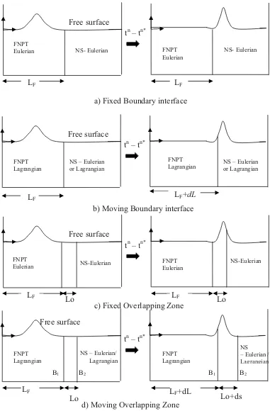
with viscous flow models. One is weak coupling and the other is strong coupling as described in Table 1. The weak coupling is faster as it needs to only transfer information in one direction and holds good for some problems. However, when carrying out the simulations for a long time wave-structure interaction, one needs to resort to a strong coupling procedure in which the information from both the solvers is exchanged, and so solutions from both the solvers affect each other. In this paper, the strong coupling procedure is employed. In general, the strong coupling needs to couple the models both in space and time domains. For the coupling in the space domain, the following three methods have been found to be employed [34,41,40]:

1. Fixed boundary interface. 2. Moving boundary interface. 3. Fixed overlapping zone interface.

They are illustrated in Fig.2a, b, and c, respectively. Options 1 and 3, where the interfaces are fixed, hold good if both the solvers are based on the Eulerian formulation and fixed meshes, for example, [34] and [40]. Option 3 was also used for SPH-one way coupling [43] but they need to add or delete the particles at every time steps in the overlapping zone. In this option the conservation of mass is questionable. The second approach is potentially suitable for the Lagrangian formulation. However, if adopting this approach, one may have difficulty in satisfying the conditions on the moving interface. That is because the conditions and variables to be solved are different on the different sides of the interface as the fluid flow is potential in one region and viscous in other region.

Fig.2c is that the overlapping zone is allowed to move and its boundary is allowed to vary. More detailed discussions about this will be given below.

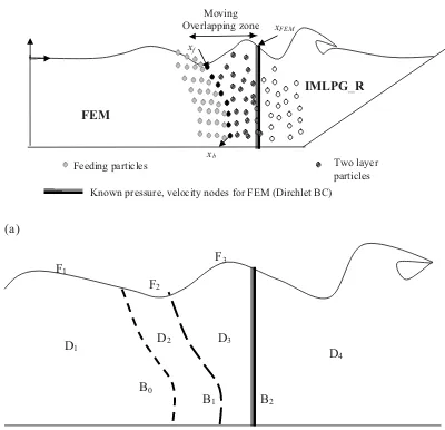
2.4.1. Moving Overlapping zone

As it has been described above, the whole computational domain is split into two sub-domains, one where the FNPT-based finite element method applies and the other where the NS-based IMLPG_R method is employed. For simplicity, the two regions will be denoted by FEM and IMLPG_R, respectively. In the FEM region, there will be no wave breaking or overturning. The technique of moving overlapping zone illustrated in Fig.2d will be adopted to couple the two solvers. It is further depicted in Fig.3 to show that the overlapping zone does not only move but its shape also varies during simulation. The FNPT model is applied in the region up to B2 with B2 as its boundary, while the NS model is applied in the region after B1 with B1 as its boundary. B2 moves with a water particle on the free surface and is kept as straight. B1 varies with particles on it and so can be curved. The solution from the FNPT model is feed to the NS model through B1 while the solution from the NS model is feedback to the FNPT model through B2. The following three issues are needed to be addressed.

1. Treatment of FEM boundary (B2) in the IMLPG_R domain. 2. Treatment of IMLPG_R boundary (B1) in the FEM domain. 3. Treatment of the velocity in the overlapping zone.

2.4.1.1. Treatment of FEM boundary in IMLPG_R domain

The information on the FEM boundary B2 must be obtained from the solution of the IMLPG_R method. The difficulty is that the unknown variable to be solved in the FEM is the velocity potential and so the boundary value on B2 should be given in terms of the velocity potential, whereas the IMLPG_R method can only provide the solutions for velocity and pressure. In addition to this, the nodes for the FEM are generally not coincident with the particles for the IMLPG_R method. If B2 follows the particles used for the IMLPG_R method, large deformation of elements for the FEM may occur and so cause numerical problems. To avoid this, it is proposed that the B2 boundary is kept to be straight and vertical and move horizontally with a particle on the free surface, similar to that for dealing with the radiation boundary in [4, 7]. The positions of nodes on B2 for the FEM calculation and the value of velocity potential on them is estimated by the following equations

R IMLPG x_f

u

dt

dx

_ &

R IMLPG

w

dt

dz

Fig.2 Different space coupling approaches. d) is the new one adopted in this paper. ( LF is the initial length

of the FNPT domain, and Lo is the initial length of the overlapping zone. dL and ds are the distances

varying with time.)

Free surface

NS- Eulerian

tn – tn*

NS- Eulerian

Free surface

tn – tn*

FNPT

Lagrangian NS – Eulerian _{or Lagrangian}

LF LF

LF LF+dL

a) Fixed Boundary interface

b) Moving Boundary interface

Free surface

tn– tn*

FNPT Eulerian

NS-Eulerian

Free surface

FNPT Lagrangian

tn – tn*

LF LF

LF _LF+dL

c) Fixed Overlapping Zone

d) Moving Overlapping Zone

Lo Lo

Lo Lo+ds

NS – Eulerian / Lagrangian NS – Eulerian

or Lagrangian

NS-Eulerian

NS – Eulerian/ Lagrangian

FNPT Lagrangian FNPT

Eulerian FNPT Lagrangian

FNPT Eulerian FNPT

Eulerian

(a)

Fig 3b. Details of the computation domain and boundary descriptions used in the hybrid model (D : Domain, B: Boundary, F: Free surface boundary)

Fig.3. Illustration of Coupling technique - moving overlapping zone

gz

u

u

u

P

dt

¸

¹

·

¨

©

§

)

w

_ 2

.

2

1

2

*

(25b)

where P is the dynamic pressure, the subscript IMPPG_R refers the variables calculated by using the solution of the IMPPG_R method, xf corresponds to the free surface node on

IMLPG_R FEM

Feeding particles Two layer

particles

Known pressure, velocity nodes for FEM (Dirchlet BC)

xFEM

xb

xf

Moving Overlapping zone

D1

D2 D3

D4 F1

F2

F3

B1 B2

B2 and uf corresponds to the velocity of the nodes used for the FEM and calculated by using ((x&n x&n1)/dt), with n referring to current time step. It is noted that the reason for the term with uf to be considered is because the nodes on B2 have normally different velocity from

R IMLPG x_f

u

_

& _.

As indicated above, the nodes for the FEM is generally not coincident with the particles for the IMPPG_R. As a result, the pressure and velocity for Eq. (25) need to be interpolated from the IMLPG_R solution. The interpolation scheme used for this purpose is based on the moving least square (MLS) scheme as described in [46]. One point is just noted here. If the total pressure from IMLPG_R method would have been used in Eq. (25), the oscillation in pressure is severe for a long time computation. This problem was also noticed and reported by Sueyoshi et al. [40] when coupling the BEM method with the MPS method in their work. That is why only dynamic pressure is estimated from the IMLPG_R solution but the static pressure is added explicitly in Eq. (25).

2.4.1.2. Treatment of IMLPG_R boundary in the FEM domain

For the IMLPG_R boundary (B1), similar issues to those discussed for B2 above need to be addressed, that is how to move the particles and how to determine the values of physical variables on B1, though the way to deal with them must be different. As for moving particles on B1, the consideration should be given that the IMLPG_R method is based on the fully Lagrangian formulation, and so the position of a particle is determined by the fluid velocity. In water waves, the fluid velocity on the free surface is generally much larger than that at the bottom, though the difference becomes smaller in shallow water cases. In our research, tests have been carried out to use the straight line for B1 and move it in the similar way as for B2. When doing so, one needs to add and delete particles for the IMLPG_R method as what had been done by Kassiotis et al. [43] for dealing with inlet and outlet boundaries of their SPH method. It is found that large error can occur due to lack of mass conservation. We instead propose another approach here, that is, the particles on B1 are always kept on it, and so the shape of B1 is determined by the position of the particles, whose velocity is determined by interpolating the velocity based on the solution in the FEM domain using the method detailed in [10]. As the particles’ velocity is equal to fluid velocity, the B1 generally becomes curved during simulation even though it may be selected as a straight line at start. The curved line will always be single valued as waves will not be overturned (so not broken) in the FEM region before B2 as indicated above. With this approach, the particles for the IMLPG_R method will never move out the region for it, and so there does not exist the issues of mass non-conservation. However, it is noted here that the velocity of particles on B1 determined in this way may not be continuous with the velocity at the particles in the IMLPG_R region. This issue will be addressed in the next section.

the pressure gradient near B1 is necessary in order to evaluate the velocity of particles within the IMLPG_R domain.

The pressure at the particles on the IMLPG_R boundary B1 is determined by Eq. (6), i.e.

gz

u

u

dt

d

P

FEM

B

¸

¹

·

¨

©

§

)

&

_˜

&

2

1

1 (26)

where the subscript FEM indicates that the values are estimated by using the solution in the FEM domain. Again the hydrostatice pressure is directly evaluated by the position of the particle concerned. There are two issues associated with the evaluation in Eq. (26). The first one is how to determine the time derivative of the velocity potential. Although it may be theoretically estimated by a finite difference scheme from the solution of two successive time instants in the FEM domain, it has been well known that using this way may cause instability [2]. In this paper, the time derivative of the velocity potential is

found by solving a boundary value problem for

dt

d)

, formed by Laplace equation and

Neumann boundary conditions on wave paddle and bottom, and Dirchlet boundary conditions on the free surface and B2, similar in some way to those in Eqs. (1)-(6) for finding the velocity potential. More details about this can be found in [4,5,10]. The second issue is that solutions for the velocity potential and its derivatives in the FEM domain are given at the nodes for the FEM method but the pressure needs to be evaluated at the particles for the IMLPG_R method. They are not at the same positions as indicated

above. Because of this, the velocity and the values of

dt

d)

for the IMLPG_R particles

are estimated from the FEM solution using the interpolation scheme mentioned for Eq. (25).

The pressure gradient for computing the velocity within the IMLPG_R domain can be evaluated by using the simplified finite difference scheme (SFDI) [49] from the solution of pressure in the IMLPG_R domain. The problem is that this scheme is based on a local support domain associated with each particle. For a particle near B1, its local support domain may go outside of the IMLPG_R domain. To evaluate the pressure gradient more accurately, several layers of imaginary particles, called as ‘Feeding particles’ are added to the left of B1 as shown in Fig. 3. The domain associated with the feeding particles is called as D2 and its upstream and downstream boundaries are B0 and B1, respectively. The position of the particles is determined by using the velocity from the solution in the FEM domain. The pressure values at the feeding particles are estimated in the same way as for finding the pressure of the particles on B1 given in Eq. (26), i.e., also from the FEM solution. Based on our experience, at least four layers of feeding particles are required. In our test cases reported latter, ten layers of feeding particles are used to model the steep wave cases.

2.4.1.3. Treatment of the velocity in the overlapping zone

updated. This involves the need of velocity estimation, which can be calculated from the velocity potential in the domain (D1 and D2) and from pressure in D4 (Fig. 3b). The dilemma exists in the overlapping zone (D3). Within the overlapping zone, there are nodes for the FEM method and particles for the IMLPG_R method. The velocity field within this zone determined by the solution in the FEM domain may not be exactly the

same as that determined by the solution in the IMLPG_R domain. Considering this fact, the particles in this region of the IMLPG_R zone are called ‘two layer particles’ (TLP). As long as there are no broken waves in the zone, the viscous effect may not play an important role and so both solutions should be close to each other. Nevertheless, use of either one will lead to discontinuity across boundaries B1 and B2. Even the quantity of discontinuity is small, the spurious high frequency wave components can be induced as quoted in [40]. To overcome this difficulty, it is proposed to smooth the velocity in the overlapping zone before updating the free surface and the position of particles for the IMLPG_R method. Specifically, the velocity at the two layer particles in the overlapping zone (D3) is modified using the following equation:

R IMLPG FEM

p u u

u (1 ) _

& &

& _{D D}

(27)

where D is given by

) , min( , 1 / 0 1 / 0 , 2 sin 1 0 / 1 _ _ 0 0 0 0 0 b f R IMLPG p FEM R IMLPG FEM x x x x x s x x L L s L s L s L s ° ° ¯ ° ° ® ­ t » ¼ º « ¬ ª d S D

where, xFEM,, xf and xb, are depicted in Fig. 3., and xp is the coordinate of the particle under considerations inside the overlapping zone. The velocity u&_FEM at the particles for the IMLPG_R method is obtained by interpolating the solution of the FEM method using the MLS scheme mentioned already.

2.4.2. Coupling methods in time domain

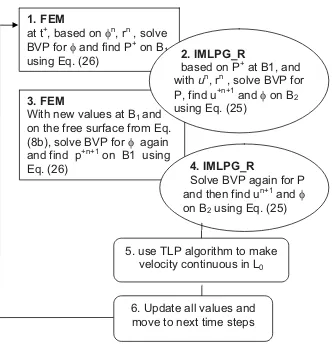
with the predictor-corrector algorithm as shown in Fig. 4. This is a kind of implicit coupling.

Fig.4. Flowchart of the coupling adopted in time.

From the figure, one could see that the IMLPG_R solver needs to be invoked twice in each time step. Following Sriram and Ma [27], the fluid particle positions were unchanged during each time step. This is justified by the fact that the movement of the node is very small in one time step and so change of particle positions caused by the deformation of the domain interface in one step is negligible. Our numerical tests indicate that the solution found in this way is much more stable than those if the particle positions are allowed to vary during predictor-corrector step. In addition, keeping the fluid particle position unchanged has the following advantages:

1. FEM

at t+, based on In, rn , solve BVP for I and find P+ on B1 using Eq. (26)

3. FEM

With new values at B1and on the free surface from Eq. (8b), solve BVP for I again and find p+n+1 on B1 using Eq. (26)

2. IMLPG_R

based on P+ at B1, and withun, rn , solve BVP for P, find u+n+1 and I on B2 using Eq. (25)

4. IMLPG_R

Solve BVP again for P and then find un+1 and I on B2 using Eq. (25)

6. Update all values and move to next time steps 5. use TLP algorithm to make

1. Matrix A in Eq. (24) remains unchanged. The computational time in re-assembling the ‘A’ matrix during the correction step is not required.

2. In our IMLPG_R method, the pressure equations are solved using an iteration solver like GMRES and Gauss-Seidel. Hence, with an unchanged matrix A, the number of iterations required for solving the pressure equations will be minimized.

More discussion on the procedure in Fig.4 is given here. Say at a particular time, ‘tn’, the simulation from both the computational domains is finished and the value of velocity potential (I), time derivative of potential (dI/dt) velocity, pressure and nodal positions are known at the free surface and boundaries. Then the simulation from ‘tn’ to ‘tn+1’ follows the 7 stages of calculation below, referring to Fig. 3b and 4:

1. The computation in the FEM domain:

a) Solve the BVP for the potential (In) using Eq. (7) on the D1, D2, D3with the known values at F1,F2,F3and B2from the previous time step.

b) Solve the BVP to find (dI+n/dt) on D1, D2 and D3.

c) Estimate the intermediate pressure on B1 (Eq. 26) , B0 and D2 (Eq. 6) as well as the velocity in D2 from the FEM solution.

2. Prediction computation in the IMLPG_R domain:

a) Solve the BVP about the pressure in D3 and D4, with Dirchlet boundary condition on B1.

b) Find the intermediate velocity in D3 and D4 [Eq. (19)] with the help of ‘Feeding particles’ in D2.

c) Transfer the data to the nodes on the boundary B2 for the FEM. Evaluate dynamic pressure using the SFDI scheme.

d) Calculate the value of the velocity potentialon B2 using Eq. (25). 3. Intermediate updating in the FEM domain and re-computation:

a) Evaluate the intermediate co-ordinates and potential using Eq. (8b) on F1,F2 and F3 and then solve the BVP for the new potential In+1.

b) Solve the BVP to find (dI(n+1)/dt).

4. Estimate the pressure on B0 , B1 and in D2 as well as the velocity in D2 from the FEM solution; then transform them to the IMLPG_R particles on B1 and on the feeding particles.

5. Correction computation in the IMLPG_R domain:

a) Re-solve the BVP about the pressure in D3 and D4.

b) Find the velocity in D3 and D4 with the help of ‘Feeding particles’ on D2. c) Transfer the data to the nodes on B2 for the FEM using Eq. (25).

6. Modify the velocity in D3 using the algorithm (Eq. 27).

7. Full updating in both domains

a) Evaluate r&n+1 and In+1 using eqn. (8d) on F1, F2 and F3 for the FEM domain.

3.0 Validation and Numerical Results

In this section, the newly developed method will be validated and its properties (overlapping zone effect, convergent features, computational costs and so on) will be discussed by applying it to model various types of waves.

3.1. Wave profile smoothness

A key question about the developed method needs to be answered, that is whether or not the hybrid method can correctly yield the smooth wave profile across the coupling zone. To test this, the method is applied to modelling the waves with the small steepness. They are generated by a piston-type wave maker that is subjected to the motion defined by the following equation

)) cos( 1 ( )

(t S0 t

S Z (28)

with the amplitude of S0 = 0.0064m and frequency (Z ) of 4.5415 rad/sec. To simulate this case, a tank with a total length (L) of 14m (Fig.2) is considered, in which the FEM computational domain length (Lf) is 3m and the IMLPG_R computational domain length is (Lm) is 12m. The initial overlapping zone width (Lo) is 1m, as shown in Fig. 5 by the two vertical solid lines. The evaluation of the initial overlapping zone width will be discussed later. At the far end of the tank, a wave damping zone is added to reduce the reflection from it as in [46]. In this zone, the velocity is modified by adding an artificial damping term and computed by usingu&n1 u&*u&**v(x)u&n1, in which v(x)is an artificial damping coefficient defined as,

d dm

d

x x L

x x v

x

v _» t

¼ º «

¬ ª

¸¸¹ · ¨¨©

§

cos ( )

1 2 1 )

( 0

S

(29)

0 2 4 6 8 10 Length of the tank (m)

-0.015 -0.01 -0.005 0 0.005 0.01 0.015

K

(m

)

0 2 4 6 8 10

Length of the tank (m) -0.015

-0.01 -0.005 0 0.005 0.01 0.015

K

(m

)

0 2 4 6 8 10

Length of the tank (m) -0.015

-0.01 -0.005 0 0.005 0.01 0.015

K

(m

)

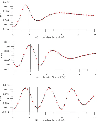
Fig 5. Comparison between analytical (Red triangles) and numerical (dotted lines) spatial wave profiles at

different time instants a) t = 2s b) t = 4 s and c) t = 8 s. The two vertical lines show the initial width of the

overlapping zone. The result to the left are from the FEM and to the right are from the MLPG_R.

(b)

These locations are just before and after the overlapping zone location, respectively. The figure again shows an excellent agreement between the analytical and numerical simulation with the maximum relative error being 1.23e-4.

0 2 4 6 8

time (s) -0.015

-0.01 -0.005 0 0.005 0.01 0.015

K

(m

)

(a)

0 2 4 6 8

time (s) -0.015

-0.01 -0.005 0 0.005 0.01 0.015

K

(m

)

(b)

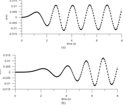
Fig 6. Comparison between analytical and numerical wave elevation time histories a) at x = 1m in the FEM domain and b) x = 4m in the MLPG_R domain (refer Fig. 5 for location).

3.2. Error Analysis

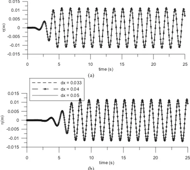
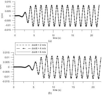
particles of 20910, 14976, 9681 respectively) but keeping a fixed time step of 0.01s. The results of wave elevation time histories are shown in Fig. 7, which are recorded at two different locations, one before the overlapping zone and one after the overlapping zone. The figure shows that the results corresponding to different numbers of particles have very small differences. Taking this as a basis, the simulations are secondly carried out for various time steps (0.02s, 0.01s and 0.006667s) with the constant spacing of 0.04m (or the number of particles being 14976). The variation of the time steps may be represented by the ratio of dx/dt, following our previous work [26, 27], which is 2 m/s, 4 m/s and 6 m/s, respectively, corresponding to the above time steps. The wave time histories recorded at the same locations as in Fig. 7 are given in Fig. 8. Again, the agreements between the results seem to be excellent.

0 5 10 15 20 25

time (s) -0.015

-0.01 -0.005 0 0.005 0.01 0.015

K

(m)

(a)

0 5 10 15 20 25

time (s) -0.015

-0.01 -0.005 0 0.005 0.01 0.015

K

(m

)

dx = 0.033 dx = 0.04 dx = 0.05

(b)

Fig 7. Comparison of wave elevation time histories obtained by using different numbers of particles a) at x = 1m b) x = 4m (refer to Fig. 5 for location).

Further, the relative error at each time step is estimated in the way similar to [27,46] by

r r c r

K K K

where A

³

r

r dA

2 K K

with Ar being the area over which the error is estimated and taken as

the whole length of the tank here; Kc _{is the computed wave profile at each time step;} Kr

is the reference solution at corresponding time instant. The reference solution in the present case is taken from the FNPT model, i.e. by running only the FNPT simulations.

0 5 10 15 20

time (s) -0.015

-0.01 -0.005 0 0.005 0.01 0.015

K

(m)

(a)

0 5 10 15 20

time (s) -0.015

-0.01 -0.005 0 0.005 0.01 0.015

K

(m

)

dx/dt = 2 m/s dx/dt = 4 m/s dx/dt = 6 m/s

(b)

0 4 8 12 16 20 time (s)

-15 -12 -9 -6 -3

log(

Hr

)

dx/dt = 2 m/s dx/dt = 4 m/s dx/dt = 6 m/s

(a)

0 4 8 12 16 20

time (s) -15

-12 -9 -6 -3

log(

Hr

)

dx = 0.033 dx = 0.04 dx = 0.05

(b)

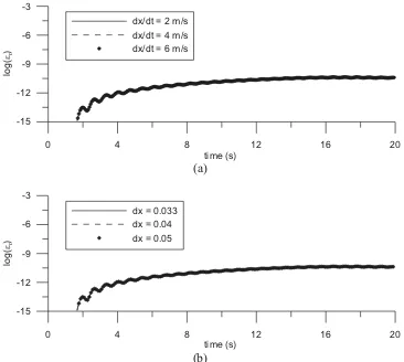
Fig 9. Relative error time histories with respect to the FNPT simulation a) by varying the distance between the nodes with constant time step (0.01s) b) by varying the time step with constant nodal spacing (0.04m).

The relative error of time histories estimated in this way are shown in Fig. 9 for the two cases corresponding to Figs. 7 and 8. From the figure, one could clearly see that the errors are less than 10-9 and tend to not increase with the time.

The errors for different values of dx/dt given in two different norms are also checked. The first is L1-error norm defined as,

¦

N

i r

L i

N E

1

1 ()

1

H (31)

where, Hr is defined in Eq. (30) and N is the total number of time steps. The second is Lf-error norm given by,

E_Lf max(H_r(i),i 1,...N) (32)

whereas, the corresponding error value of ELf are 3.406e-5, 3.278e-5 and 3.195e-5, respectively for the same cases in Fig. 9.

All the results described above indicate that results obtained by using different numbers of nodes and time steps seem to be converged. It is noted that the specific values of the relative error do not only depend on the number of nodes and the length of each time step but also on wave parameters such as wave amplitudes and periods (see Fig. 13 below), similar to those of other numerical methods.

3.3 Behaviours ofmoving overlapping zone

Another key question about the developed method needed to be answered is whether or not the moving overlapping zone in the hybrid method behaves properly. In the cases discussed above, the wave amplitude is small and so the variation of the overlapping zone is not significant. Therefore those cases do not sufficiently demonstrate the behaviours of the moving overlapping zone. In this section, the hybrid method will be applied to model the cases with larger amplitudes and larger steepness. The total length of the tank (L) is 45m with Lf, Lm, Lo taken as 6m, 40m and 1m respectively. The amplitude of the motion of the wavemaker is 0.042m and the angular frequency is 4.5415 rad/s . The time step adopted in the simulation is 0.005s (about 277 steps per wave period) and the distance between the nodes is 0.04m. The case is simulated by two ways. One is to employ the FNPT method only and the other is the hybrid method. The simulated wave profiles at different time instants from the two methods are compared in Fig. 10. From the figure, one can see that the moving overlapping zone for the hybrid method varies and moves significantly during the simulation. More specifically, the position of the moving boundary B2 (Fig. 3b) denoted by blue dots moves considerably (>25% Lo) to the right. The particles denoted by black dots on the boundary (B1) of the IMLPG_R zone (Fig. 3b) do not only move considerably but also not uniformly: more on the free surface and less near the bottom as expected (see, e.g., at t=10.5s), making the boundary curved. The configuration of feeding particles (red) also varies significantly during the simulation. In addition, the minimum width (on the free surface) of the overlapping zone evidently decrease during crest occurrence (t = 12.5s), compared to trough occurrence (t = 10.5s) in the zone. With these dynamic variations of the overlapping zone, the results of the hybrid method are very similar to these of the full FNPT method as one can see in this figure and also in Fig. 11. The latter presents the comparison of the time histories of the two methods recorded at three locations, one before the overlapping zone, the second in the overlapping zone and the third after the overlapping zone. The small area in Fig. 11b

is re-plotted in Fig. 11d to show how close they are. The maximum relative error is about

0.002.

Fig 10. Comparison of free surface profiles at different time instants. Red circles – full FNPT simulation;

Blue line – FEM domain; Color map and black line – MLPG_R domain. Columns of red particles– Feeding

0 10 20 30 time (s)

-0.08 -0.04 0 0.04 0.08 0.12

K

(m

)

0 10 20 30

time (s) -0.08

-0.04 0 0.04 0.08 0.12

K

(m

)

Fig. 11 (a) Fig. 11 (b)

0 10 time (s) 20 30 -0.08

-0.04 0 0.04 0.08 0.12

K

(m)

FNPT Present

2 4 6 8 10 12

time (s) -0.08

-0.04 0 0.04 0.08 0.12

K

(m)

Fig. 11 (c) Fig. 11 (d)

Fig 11. Comparison of wave elevation time histories produced by the hybrid method and the full FNPT

method: a) x = 4m before the overlapping zone ; b) x = 5m from wave paddle c) x = 9m after the

overlapping zone. d) an enlarged view of the boxed area in (b).

3.4. Effect of overlapping zone width

1.5TUmax, 2.0 TUmax and 2.5 TUmax, respectively,. The wave time histories recorded at two locations are shown inFig. 12. The figure shows that the results corresponding to all the three initial widths are very close. The relative error for this case is again estimated based on the full FNPT results (as in Fig. 9) and are shown in Fig. 13a. The values of E_Lf

for the three cases are 0.002029, 0.002028 and 0.002022, whereas, the values of EL1 are

0.00096, 0.00096 and 0.00099, respectively. One can see from these figures that the results corresponding to three different initial widths of the overlapping zone are very close to each other and so may conclude that they are all suitable to ensure good behaviours of the hybrid method. Based on this, 2.0 TUmax may be used for periodic waves presented in this paper. However, it should be noted that this may be case-dependent and may need to be tested for other cases. As there are two different solvers adopted, conservation of mass or volume needs to be investigated. This can be checked by the error defined as,

, ) (

0 0

m m t m Em

(33)

where, m t d dA

A

t

³

³

:

K )

(

) (

m0 is the initial domain volume. The values of the relative error in the present test cases are shown in Fig. 13b (for full FNPT and for the three different overlapping widths). The figure shows that as the time increases, the error increases slowly for all the methods but

it remains limited during the whole simulation. However, the error is a bit higher for the

present hybrid method than for the full FNPT solutions. Nevertheless, it can be considered as acceptable.

0 5 10 15 20 25

time (s) -0.08

-0.04 0 0.04 0.08 0.12

K

(m

)

Width = 0.75m(_#7umax)

Width = 1.0m(_#7umax)

Width = 1.25m(#7umax)

0 5 10 15 20 25 time (s)

-0.08 -0.04 0 0.04 0.08 0.12

K

(m)

(b)

Fig 12. Comparison of wave elevation time histories for various overlapping zone widths a) x = 4m from

wave paddle (i.e., in FNPT domain) b) x = 9m from wave paddle (i.e., in MLPG domain).

0 5 10 15 20 25

time (s) -15

-12 -9 -6 -3

log(

Hr

)

Width = 0.75m(#7umax)

Width = 1.0m(#7umax)

Width = 1.25m (#7umax)

0 5 10 15 20 25 time (s)

-15 -12 -9 -6 -3

log(

Em

)

FNPT

width = 0.75m (#7Umax)

width = 1.0m (#7Umax)

width = 1.25m (#7Umax)

Fig. 13b. Error time history of water volume for different initial widths of the overlapping zone

3.5. Effect of position of the overlapping zone

The fourth question that needs to be answered is whether or not the initial position of the overlapping zone would affect the results and how it is chosen. There are a couple of points to be considered for choosing the initial position. Firstly, the overlapping zone should be well away from the wave breaking location as the FNPT model is not suitable for such region as discussed before. Secondly, the region for the FNPT method should be as large as possible in order to reduce the region of NS domain and help saving the computational time. It is expected that the initial position of the overlapping zone has a little effect on the results if the first point is met. In this section, the hybrid method is further investigated to confirm that the initial position of the overlapping zone does not significantly affect the simulation results. For this purpose, the simulations have been carried out for various cases with regular and solitary waves but only the results for the solitary wave are discussed in this sub-section. Nevertheless, the conclusion regarding the influence of the initial position of the overlapping zone is held the same for other cases considered.

The solitary wave is generated by a piston-type wavemaker according to the theory given by Goring [51], in which the motion of the wavemaker is defined by

>

@

k H

x_p(W) tanhF( )tanh O/

(34)

where H is the wave height (taken as 0.3m) above the rest water level, k 3H/4h,

>

@

k _p( ) /

)

(W W O

F _{and the celerity} c gh(1H/h)

domain. As for selecting the overlapping zone width, the methodology suggested in the previous section (TUmax) is not applicable for solitons as the wave period is theoretically infinite long. Hence, another simple approximation for solitary wave is considered using the maximum wave paddle displacement (_xpl_), where _ xpl _ is estimated by 0.5_ xpl _ #

H/k. Similar tests considering 1.5_xpl_, 1.75_xpl_and 2_xpl_ have been carried out, and all of them have almost the same results. Based on this, the overlapping zone width is taken as 1.0m, which corresponds to 1.75_ xpl_. The simulation for the cases with different initial positions of the overlapping zone is made in two ways, as referred to Fig. 14. One is to employ the full FNPT method and the other is the hybrid method. The time histories are recorded at 3m and 8m from the wave paddle and presented in Fig. 14. The first location corresponds to the one before the overlapping zone (in the FEM domain) and the other after the overlapping zone (in the MLPG_R domain). One can observe from the figure that all the results from the hybrid method with different initial positions of the overlapping zone are almost the same as these produced by the full FNPT method. The maximum relative errors between the results of FNPT method and the hybrid method with different initial positions (4m, 5m and 6m) of the overlapping zone are 0.01068, -0.01007,-0.008 respectively.

0 2 4 6 8

time (s) -0.1

0 0.1 0.2 0.3 0.4

K

(m

)

Hybrid, Lf = 4m Hybrid, Lf= 5m Hybrid, Lf= 6m FNPT

0 2 4 6 8

time (s) -0.1

0 0.1 0.2 0.3 0.4

K

(m

)

Fig 14. Comparison of wave elevation time histories of two methods- full FNPT and hybrid method: a) at x = 3m and b) x = 8m from the wave paddle.

3.6. Validation against experimental results

Cnoidal waves that are highly nonlinear. The experiments are carried out in a tank of 110m long with a water depth of 0.62m in Franzius Institute, University of Hannover, Germany. In the numerical modelling, the total length of the tank (L) is 76m with the length of the FEM domain (Lf) being 33m and the MLPG_R domain length (Lm) being 44m. The total number of nodes used on the free surface and along the depth of the tank for the FNPT method is 701 and 17, respectively, whereas the initial distance between the particles in the MLPG_R domain is taken as 0.041m. The time step adopted for the simulation is 0.01s (about 660 time steps per wave period). The motion of the wave paddle is shown in Fig. 15a and is the same as in the experiment. Fig.15b, c and d show the wave time histories recorded at two positions in the FEM domain and at the two positions in the MLPG_R domain. They are all compared with the corresponding experimental measurements. The figure shows a good agreement between the experimental results and those from the present numerical model. In particular, it even quite accurately captures the high frequency components in the wave profiles. Overall, the maximum relative error between the numerical and experimental measurements is 0.03. Nevertheless, there are some small differences between them after 40s. One of reasons for the difference may be because of the different absorbing zone effects in experiments and in numerical modelling, as reported in [47]. The absorbing beach in the experimental wave flume is tested for 0.8m water depth under regular wave conditions and it does not holds good for shallow water after a long time wave generation due to reflection from the beach and in the absence of active wave paddle absorption. In the numerical modelling, the absorbing zone length is 3m, which is set based on the tests for regular waves and may need to be tuned for the Cnoidal waves. Nevertheless, the comparison evidences that the hybrid method can yield satisfactorily results with experimental data even when the waves are highly nonlinear.

0 10 20 30 40 50

time (s) -0.4

-0.2 0 0.2 0.4

S

(m

)

a)

(a)

0 10 20 30 40 50

time (s) -0.1

0 0.1 0.2

K

(m

)

Present method Experiments

b)

0 10 20 30 40 50

time (s) -0.1

0 0.1 0.2 0.3

K

(m

)

c)

(c)

0 10 20 30 40 50

time (s) -0.1

0 0.1 0.2 0.3

K

(m

)

d)

(d)

0 10 20 30 40 50

time (s) -0.1

0 0.1 0.2 0.3

K

(m

)

e)

(e)

Fig 15. Comparison of wave time histories with experimental data: a) experimental paddle motion, Sriram et al., [47] b) x = 20.146m from the wave paddle. c) x = 30.425m from the wave paddle. d) x = 40.406m

from the wave paddle. e) x = 50.609m from the wave paddle.

nodes in the MLPG_R domain is taken as 0.025m and the time step adopted is 0.005s. The spatial wave profiles of the overtopping and experimental measurements [52] are provided in non-dimensional form in Fig. 16b. The normalized dynamic pressure time histories at different locations are plotted in Fig. 16c. The figure shows a reasonable agreement between the results from the numerical modelling and from the measurements. As the present numerical model is based on single phase flow, the air entrapment behind the seawall noticed in the experiments is not properly re-produced. The dynamic pressure time histories shown in Fig.16c are quite smooth, and compare well with experimental data.

In the third case for the validation, the hybrid method is applied to model a more violent solitary wave. The results are compared with the experimental data from Li and Raichlen [53]. In this case, a solitary wave propagates over a beach with a slope of 1:15. The solitary wave is again generated by a piston-type wavemaker according to the theory given by Goring [51] as described above but the wave height is taken as 0.45m above the rest water level with the water depth being 1m over the flat bed spanning 6m from the wavemaker to the toe of the slope beach. The example is similar to that used in Sriram and Ma [27]. In the simulation, the total length of the tank (L) is 21m, in which the FEM domain length is 12.8m and the MLPG_R domain length is 8.2m. The number of free surface nodes in the FEM domain is 401 and in vertical direction it is 17, whereas in the MLPG_R domain the initial distances between the particles are selected as 0.025m and the time step is taken as 0.0032s. Sriram and Ma [27] and Ma and Zhou [26] have shown that these parameters are appropriate to give convergent results. The initial configuration and numerical setup is shown in Fig.17a. The snapshots of the free surface profiles and the configuration of water particles at various time instants are shown in Fig.17 b-e, together with the experimental data from Li and Raichlen [53] (in red line). The time has been reported in a non-dimensional form (t gd ). Again, a reasonable agreement between the numerical simulation and experimental profiles are observed. Fig.17f – g, shows the snapshot of the profile after breaking, in which the smooth profiles of pressure are observed.

Fig.16a. Initial configuration of the numerical simulation for solitary waves overtopping a seawall (contour map indicated the pressure in the MLPG_R domain).

`

Fig.16b. Comparisons of free surface elevations obtained by experiments [52] (left column) and numerical simulations (right column). Numerical free surface at t = (a) 4.424, (b) 4.92, (c) 5.03, (d)5.15, (e) 5.27, (f) 5.85;.Experimental data [52]()

(e) (c) (b)

(d)

2 4 6 8

t—gd

0 0.0001 0.0002 0.0003 0.0004 Pd / U gd

2 4 6 8

t—gd

0 0.0001 0.0002 0.0003 0.0004 Pd / U gd

2 4 6 8

t—gd

0 0.0001 0.0002 0.0003 0.0004 Pd / U gd

2 4 6 8

t—gd

-0.0001 0 0.0001 0.0002 0.0003 0.0004 Pd / U gd

2 4 6

t—gd

0 0.0001 0.0002 0.0003 0.0004 Pd / U gd

2 4 6

t—gd

0 0.0001 0.0002 0.0003 0.0004 Pd / U gd P1 (14.2,0.73)

P3 (14.5, 0.8)

P7 (14.85, 0.9) _{P10 (15.57, 0.92)}

P11 (15.67, 0.85) P12 (15.7, 0.84)

Fig.16c. Comparison of the pressure time histories between numerical (line) and experimental

measurements [52]().The pressure locations (P1, P3, P7, P10, P11, P12) correspond to experimental measurements [52] are illustrated in top figure with black dots.

P1

P3 P7 P10P11

3.7. Computational costs

As indicated before, one of the important reasons to develop the hybrid method is that it is computationally more efficient. To demonstrate this, a series of test cases with different lengths for the FEM and IMLPG_R regions for the same total length of the tank as that for Fig. 17 has been considered as given in Table 2 in order to get the optimum

computational costs for the cases. Domain I corresponds to use of the IMLPG_R method

in the whole domain. All the computations are carried out on a DELL E4200 Laptop having a 1.2GHz processor with 2.95GB RAM, using the same node spacing and time step as reported in Section 3.6. The wave time histories at two different locations for the different cases are shown in Fig. 18a-b. The time history just before the wave overturn, i.e. near very steepest point is reported for all the cases. This is indicated by almost a straight profile in the time history, as denoted by the red line on Fig. 18b. All the figures show almost identical results, confirming again that the coupling location does not have influence on the results even for very steep or overturning waves. From Table 2, it can be seen that the shortest CPU time is 1 hrs 9min, which corresponds to the case with longest domain for the FEM as expected. If further increasing this domain, the computational time will be reduced again but the results will be incorrect as it will cover the wave broken region where the FEM should not be employed as indicated above. In addition, for the case corresponding to Fig. 16, the hybrid method took 2 hrs 56mins, in contrast to 10 hrs 25mins taken by the full IMLPG_R model on the same computer. Thus, one again clearly sees a significant decrease in computational time using the present approach.

(a)

(b) a)

b)

(c)

(d)

(e)

(f)

time = 11.15 c)

d)

e)