An efficient indirect RBFN-based method for numerical solution of PDEs

An Efficient Indirect RBFN-Based Method for

Numerical Solution of PDEs

Nam Mai-Duy

_{and Thanh Tran-Cong}

a

_{School of Aerospace, Mechanical and Mechatronic Engineering,}

The University of Sydney, NSW 2006, Australia

b

_{Faculty of Engineering and Surveying,}

The University of Southern Queensland, Toowoomba, QLD 4350, Australia

Submitted to

Numerical Methods for Partial Differential Equations

23 December 2003, revised 8 November 2004

Abstract This paper presents an efficient indirect radial basis function network

(RBFN) method for numerical solution of partial differential equations (PDEs).

Previous findings showed that the RBFN method based on an integration process

(IRBFN) is superior to the one based on a differentiation process (DRBFN) in

terms of solution accuracy and convergence rate [1]. However, when the problem

dimensionalityN is greater than 1, the size of the system of equations obtained in the

former is aboutN times as big as that in the latter. In this paper, prior conversions

of the multiple spaces of network weights into the single space of function values

are introduced in the IRBFN approach, thereby keeping the system matrix size

small and comparable to that associated with the DRBFN approach. Furthermore,

the nonlinear systems of equations obtained are solved with the use of trust region

methods. The present approach yields very good results using relatively low numbers

of data points. For example, in the simulation of driven cavity viscous flows, a high

Reynolds number of 3200 is achieved using only 51×51 data points.

Keywords radial basis function, trust region methods, Poisson equation,

1

Introduction

The finite difference method (FDM) (cf. [2]), the finite element method (FEM) (cf.

[3]), the finite volume method (FVM) (cf. [4]) and the boundary element method

(BEM) (cf. [5,6]) are powerful techniques for numerical solution of boundary-value

problems in continuum mechanics. Each method has some advantages over the

oth-ers in certain classes of problems. They have achieved a lot of success in solving

engineering and science problems. However, since their approximations to the

gov-erning equations and boundary conditions are usually based on low order schemes

such as constant, linear and quadratic ones, dense meshes are required for a high

degree of accuracy. On the other hand, the spectral method (cf. [7,8]), the

differ-ential quadrature method (cf. [9]) and the radial basis function network (RBFN)

based method (cf. [10]) fall under the category of high order methods by which

ac-curate results can be obtained using relatively coarse discretizations of the domain

of interest.

The concept of solving PDEs by using RBFNs was first introduced by Kansa [10]. A

further distinguishing feature of the methods based on the neural network

method-ology is that no mesh is required. The methods use approximators based on RBFNs

to represent the solution via a point collocation mechanism. The difference between

the RBFN and spectral collocation methods is that collocation points are chosen as

the roots of the base functions (Chebychev polynomials) for the latter but can be

chosen randomly for the former. In this sense, RBFNs are comparatively easy to

implement especially for problems with complex geometries or with governing

differ-ential equations involving complicated operators. It has been proven that RBFNs

with one hidden layer are capable of universal approximation [11,12]. Although

RBFNs have the ability to represent any continuous function to a prescribed

remain an open problem. For example, due to the lack of theory, it is still very

dif-ficult to choose the optimum values of RBFN parameters such as the RBF’s widths

(shape parameters), which are seen to critically affect the performance of RBFNs.

That could be a reason why the RBFN-based methods have not been extensively

used to solve practical problems.

In an RBFN-based method, each dependent variable and its derivatives are expressed

as linear combinations of basis functions which are associated with the same set of

network weights. There are two basic approaches for obtaining new basis functions

from RBFs. The first approach, namely the direct RBFNs (DRBFNs), is based

on a differentiation process [10], while the second approach, namely the indirect

RBFNs (IRBFNs), is based on an integration process [1]. The two approaches were

tested with the solution of elliptic DEs and the IRBFN method was found to be

more tolerant than the DRBFN method in the choice of the RBF’s widths [1]. The

IRBFN method was then extended successfully to simulate the driven cavity viscous

flows with the Reynolds number achieved up to 400 using a uniform set of 33×33

data points [13]. A formal theoretical proof of the superior accuracy of the IRBFN

method has not been given at this stage. However, a heuristic argument can be

presented as follows. In the direct approach, the starting point is the decomposition

of the original function into some finite basis and all derivatives are subsequently

obtained by differentiation. Any inaccuracy in the assumed decomposition is badly

magnified in the process of differentiation. In contrast, in the indirect approach, the

starting point is the decomposition of the highest derivatives into some finite basis.

Lower derivatives and finally the function itself are obtained by integration which

has the property of damping out or at least containing any inherent inaccuracy in

the assumed shape of the derivatives.

A disadvantage of the IRBFN approach is that when the problem dimensionalityN

is aboutN times as big as that in the DRBFN approach. The increase in size of

the unknown network weights in the indirect approach is primarily due

to the fact that there areN radial basis function networks associated with

N coordinates to be used in representing each dependent variable and its

derivatives. Consequently, some additional constraints are necessary to

make the formal function representations identical [1]. In this paper, the

multiple spaces of network weights, which are unknowns here, are converted into the

single space of function values, resulting in a square system of equations with usual

size and hence greatly reducing computational effort and storage for the IRBFN

method.

For nonlinear problems, it is well known that the Newton iteration method is often

used for efficient convergence of a numerical scheme. The method possesses local

q-quadratic convergence provided that an initial guess for the iteration is close to the

desired solution. In the case that the iteration process is not started sufficiently close

to the desired solution, the Newton method needs be hybridized with a globally, yet

typically slowly, convergent Cauchy method (steepest descent) in order to construct

a globally convergent variant. The resulting so-called model-trust region algorithms

retain the best features of both methods: strong global convergence coupled with

rapid local convergence (i.e. they are globally q-quadratically convergent) [14]. In

the present work, the trust region methods are applied to solve the obtained systems

of nonlinear equations.

The present method is verified successfully through the solution of Poisson equation

and the Navier-Stokes equations. For the case of Poisson equation, highly

accu-rate results and fast convergence are obtained. For the case of the Navier-Stokes

equations, in which the benchmark problem of viscous flow in a lid-driven cavity is

simulated, the present approach yields solutions for high Reynolds numbers up to

the Navier-Stokes equations using RBF networks, this paper appears to be the first

reporting the achievement of high Reynolds number solutions.

The remainder of the paper is organized as follows. Section 2 gives brief reviews of

RBFNs and two associated DRBFN and IRBFN approaches. A new feature for the

IRBFN approach is presented in section 3. The governing equations are given in

section 4. Sections 5 & 6 discuss respectively the use of RBFNs for numerical solution

of PDEs and the use of trust region methods for solving nonlinear algebraic systems.

In section 7, the present IRBFN approach is verified through the solution of linear

heat transfer problems with the Dirichlet and Neumann boundary conditions and

the solution of non-zero Reynolds number viscous flows in a driven cavity. Section

8 gives some concluding remarks.

2

Radial Basis Function Networks

A function y to be approximated can be represented by an RBFN as follows [15]

y(x)≈f(x) =

m

X

i=1

w(i)_g(i)_{(x), (1)}

where superscripts denote elements of a set of neurons, xis the input vector, mthe

number of RBFs, {w(i)_}m

i=1 the set of network weights and {g(i)(x)}mi=1 the set of

RBFs. Since multiquadrics (MQ) are ranked the best in terms of accuracy among

RBFs [16], the present work will employ these basis functions whose form is

g(i)(x) =

q

(x−c(i)₎T_(x−c(i)_{) +a}(i)2_{, (2)}

where c(i) _{and a}(i) _{are the centre and the width of the ith MQ basis function}

simple, the centres and the widths of RBFs are chosen in advance. For the latter,

the following relation is used

a(i)=βd(i), (3) whereβ is a positive scalar and d(i) _{is the minimum of distances from the ith center}

to its neighbours.

The function y is now expressed as a weighted linear combination of radial

ba-sis functions. It can be seen that differentiating or integrating y also results in

weighted linear combinations of basis functions, where the sets of network weights

are identical.

2.1

Direct approach

In this approach, the RBF network (1) is utilized to represent the original function

y and subsequently its derivatives are computed by differentiating (1) as follows

y(x) ≈ f(x) =

m

X

i=1

w(i)_g(i)_{(x), (4)}

∂y(x)

∂xj

≈ ∂f(x)

∂xj

= ∂

Pm i=1w(

i)_g(i)_(x)

∂xj

=

m

X

i=1

w(i)_h(i)_{(x), (5)}

∂2_y(x)

∂x2

j

≈ ∂

2_f(x)

∂x2

j

= ∂

Pm i=1w(

i)_h(i)_(x)

∂xj

=

m

X

i=1

w(i)_¯h(i)_{(x), (6)}

where subscripts denote scalar components of a vector, h(i)_{(x) = ∂g}(i)_(x)/∂x

j and

¯

h(i)_{(x) =∂h}(i)_(x)/∂x

j are new derived basis functions in the approximation of first

2.2

Indirect approach

In this approach, RBFNs are used to represent the highest order derivatives of a

function y, e.g. ∂2_y/∂x2

1 and ∂2y/∂x22. Lower order derivatives and finally the

function itself are then obtained by integrating those RBFNs as follows

∂2_y(x)

∂x2

j

≈ ∂

2_f(x)

∂x2 j = m X i=1

w(i)_g(i)_{(x), (7)}

∂y(x)

∂xj

≈ ∂f(x)

∂xj

=

Z _Xm i=1

w(i)_g(i)_(x)

! dxj =

m_X+p1

i=1

w(i)_H(i)_{(x), (8)}

y(x) ≈ f(x) =

Z m_X+p1

i=1

w(i)H(i)(x)

! dxj =

m_X+p2

i=1

w(i)H¯(i)(x), (9)

where p1 and p2 are the numbers of centres used to represent integration constants

in the first and second derivatives (∂f_∂x(x)

j and

∂2f(x)

∂x2_j ) respectively (p2 = 2p1). For

convenience, these centres and their associated basis functions are also denoted by

the notations w(i) _{and H}(i) _{( ¯H}(i)_{) respectively but with i > m. For example, in}

the case of 2D problems, the integration constants in the first derivative ∂f_∂x(x)

j is

a function of the variable xk(k6=j) only and can be approximated using the indirect

RBFN approach as follows

d2_C 1(xk)

dx2

k

=

p_X1−2

i=1

¯

w(i)g(i)(xk), (10)

dC1(xk)

dxk

=

p_X1−2

i=1

¯

w(i)H(i)(xk) +Cb1 =

p_X1−1

i=1

¯

w(i)H(i)(xk), (11)

C1(xk) = p_X1−2

i=1

¯

w(i)_H¯(i)_(x

k) +Cb1xk+Cb2 =

p1

X

i=1

¯

w(i)_H¯(i)_(x

where

H(i)(xk) p1−2

i=1 =

Z

g(i)(xk)dxk

p1−2

i=1

, H¯(i)(xk) p1−2

i=1 =

Z

H(i)(xk)dxk

p1−2

i=1

,

H(p1−1)_(x

k) = 1, H¯(p1−1)(xk) = xk, H¯(p1)(xk) = 1,

¯

w(p1−1) _=Cc

1 and w¯(p1) =Cc2.

The detailed implementation was reported previously in [17]. In the present

work, the new centres in the approximation of integration constants (e.g.

C1(xk)) are chosen to be distinct xk coordinates of data points.

Several basis functions in both DRBFN and IRBFN approaches are available in

analytic forms and they can be found in [17].

3

New feature for the indirect approach

As reviewed above, in the indirect approach, the highest order derivatives are

rep-resented by RBFNs. Subsequently, lower order derivatives and the function are

obtained by integrating the RBFNs. For the approximation of a function of two

or more variables, there are a number of expressions obtained to represent a target

function since different starting points can be employed by virtue of the definition of

partial derivatives. Thus, it is necessary to impose some constraints on the function

networks in order to make the formal function representations identical [1].

The indirect approach for 2D problems can be recaptured as follows

∂2_f(x)

∂x2 1

→ ∂f(x)

∂x1

→f[x1](x), (13)

∂2_f(x)

∂x2 2

→ ∂f(x)

∂x2

where f[x1](x) and f[x2](x) are two closed-form representations for the function y

corresponding to the two starting points ∂2_{f /∂x}2

1 and ∂2f /∂x22 respectively. Since

f[x1](x) and f[x2](x) represent the same function, they must be identical, leading to

the following constraint equation

f[x1](x) =f[x2](x) = f(x). (15)

Functions in (13)-(15) can be written as linear combinations of basis functions as

follows

m

X

i=1

g(i)_(x)w(i) [x1] →

m_X+p1

i=1

H_[(_xi)_1](x)w_[(_xi)_1]→

m_X+p2

i=1

¯

H_[(_xi)_1](x)w_[(_xi)_1], (16)

m

X

i=1

g(i)(x)w(_[xi)_2] →

m_X+p1

i=1

H_[(_xi)_2](x)w_[(_xi)_2]→

m_X+p2

i=1

¯

H_[(_xi)_2](x)w_[(_xi)_2], (17)

m_X+p2

i=1

¯

H_[(_xi)

1](x)w (i) [x1] =

m_X+p2

i=1

¯

H_[(_xi)_2](x)w_[(_xi)_2], (18)

where subscripts [xi] denote the results obtained by the integration with respect to

the xi direction. The evaluation of (16)-(18) at a set of collocation points {x(j)}nj=1

yields the system of equations of the form

f,11(x) =G(x)w[x1] → f,1(x) = H[x1](x)w[x1] →f[x1](x) = H¯[x1](x)w[x1], (19)

f,22(x) =G(x)w[x2] → f,2(x) = H[x2](x)w[x2] →f[x2](x) = H¯[x2](x)w[x2], (20)

¯

H[x1](x)w[x1] = H¯[x2](x)w[x2], (21)

whereG,HandH¯ are the design matrices associated with the approximation of

sec-ond derivative, first derivative and the function respectively;w[xi]the sets of network

weights to be found;f ={f(x(j)_)}n

j=1; f,i ={

∂f(x(j)₎

∂xi }

n

j=1 andf,ii ={

∂2_f(x(j)₎

∂x2

i }

n

j=1. For

the convenience of computation, the matrices G and H are augmented using

Obviously, the unknown vector in the indirect approach is(w[x1];w[x2];· · · ;w[xN])

in which the length of each w[xi] is (m+p2) and N is the problem

dimen-sionality. Assuming that p2 (a number of additional weights from the

approximation of integration constants) is a relatively small number, the

size of the unknown vector in the original indirect RBFN approach is

about N times as big as that in the direct RBFN approach.

This paper introduces prior conversions of the multiple spaces of network weights,

e.g. w[x1]andw[x2], into the single space of function valuesf in order to form a square

system of equations of smaller size (comparable to that associated with the DRBFN

approach), thus greatly reducing the computational effort and storage. Consider the

function networks f[x1] and f[x2] in (19) and (20) respectively. By inversion, the sets

of network weights are expressed in terms of nodal function values as

w[x1] = H¯_[−x11]f[x1]=H¯

−1

[x1]f, (22)

w[x2] = H¯−_[x1_2]f[x2]=H¯−_[x1_2]f. (23)

Substitution of (22) and (23) into the system (19)-(20) yields

f,11 =G ¯H_[−_x1_1]f → f,1 =H[x1]H¯−_[x1_1]f →f[x1]=If, (24)

f,22 =G ¯H_[−_x1_2]f → f,2 =H[x2]H¯−_[x12]f →f[x2]=If, (25)

where Iis the unit matrix.

For cross derivatives∂f2_(x)/∂x

i∂xj, it is straightforward to compute them by using

network design matrices associated with first order derivatives. Although the order

be better to take the average of the two equivalent representations

∂2_f

∂xi∂xj

= 1 2 ∂ ∂xi ∂f ∂xj + ∂ ∂xj ∂f ∂xi ,

f,ij =

1 2

H[xi]H¯

−1

[xi]

H[xj]H¯

−1

[xj]f

+H[xj]H¯

−1

[xj]

H[xi]H¯

−1

[xi]f

. (26)

It can be seen from (24)-(26) that the function and its derivatives are all expressed

in terms of the function values rather than in terms of the network weights. As a

result, the system of equations obtained is normally square with the size

being slightly smaller than that of the DRBFN method, irrespective of

the problem dimensionality. For example, in solving Poisson equation,

the sizes of the system matrices are nip×nip and n×n for the indirect

and direct approaches respectively in which nip is the number of interior

points and n the number of boundary and interior points. The

transforma-tion operatransforma-tion completely eliminates the problem of large matrix size in the IRBFN

method.

4

Governing equations

Linear Poisson equations and nonlinear Navier-Stokes equations are considered in

the present work.

4.1

Poisson equation

The linear Poisson equation takes the form

∂2_u

∂x2 1 +∂ 2_u ∂x2 2

where x = (x1, x2) is the position vector of a point in the analysis domain Ω, u is

the dependent variable and s is a known function.

4.2

The Navier-Stokes equations

In solving the Navier-Stokes equations for two dimensional flows, numerical methods

usually employ the stream function-vorticity formulation rather than the

velocity-pressure formulation. The advantages of the former over the latter are that the

number of variables is reduced to two (without pressure) and the continuity

equa-tion is automatically satisfied. However, one concern is the need to derive boundary

conditions for the vorticity. The stream function-vorticity formulation will be

em-ployed here. The dimensionless Navier-Stokes equations for steady incompressible

planar viscous flows, subject to negligible body forces, are expressible in terms of

the stream function φ and the vorticity ω as follows

∂2_φ

∂x2 1 +∂ 2_φ ∂x2 2

+ω = 0, x∈Ω (28)

∂2_ω

∂x2 1 +∂ 2_ω ∂x2 2 =Re ∂φ ∂x2 ∂ω ∂x1 − ∂φ ∂x1 ∂ω ∂x2

x∈Ω, (29)

whereRe=U L/νis the Reynolds number, in whichLis the characteristic length,U

is the characteristic speed of the flow andν is the kinematic viscosity. The vorticity

and stream function are defined by

ω = ∂u2

∂x1

− ∂u1

∂x2

, (30)

∂φ ∂x2

=u1,

∂φ ∂x1

=−u2, (31)

5

Solution of PDEs using RBFNs

Each variable and its derivatives in the governing equations can be represented by

neural networks using either (4)-(6) in the direct approach or (24)-(25) in the indirect

approach. The closed-form representations obtained are then substituted into the

governing equations and boundary conditions to discretize the system via a point

collocation mechanism. In the present work, the set of collocation points is chosen

to be the same as the set of centres, i.e. {x(i)_}n

i=1 = {c(i)}mi=1. The RBFN solution

satisfies the governing equations pointwise rather than in an average sense. In order

to form a square system, the governing equations are applied to the interior points

only.

In the indirect approach, the unknown vector contains nodal variable values, e.g. u

in Poisson equation and {φ, ω} in the Navier-Stokes equations, while in the direct

approach, the unknowns are the network weights (coefficients). However, for both

approaches, it can be seen that the determination of the unknowns is based on the

process of minimizing the following sum squared errors SSE

SSE =SSE1+SSE2, (32)

whereSSE1 andSSE2are the sums of squared errors, which are employed to ensure

that neural networks satisfy the governing equations and the boundary conditions

respectively. The form ofSSE2 depends on the problem to be solved while the term

SSE1 can be written in the general form provided that the governing equations are

given. For example, SSE1 in the IRBFN formulation takes the form

SSE1 =

nip

X

i=1

" _m X

j=1

G ¯H−_[x1_1]

[i,j]u (j)₊

m

X

j=1

G ¯H−_[x1_2]

[i,j]u

(j)_−s(x(i)₎

#2

for Poisson equation (27) and

SSE1 =

nip X i=1 { m X j=1

G ¯H−_[x1_1]

[i,j]φ (j)₊

m

X

j=1

G ¯H−_[x1_2]

[i,j]φ

(j)_+ω(i)_]}2₊

nip X i=1 { m X j=1

G ¯H−1 [x1]

[i,j]ω (j)₊

m

X

j=1

G ¯H−1 [x2]

[i,j]ω (j)₋

Re[

m

X

j=1

H[x2]H¯−_[x12]

[i,j]φ (j)_H

[x1]H¯−_[x11]

[i,j]ω (j)₋

m

X

j=1

H[x1]H¯−_[x11]

[i,j]φ (j)_H

[x2]H¯−_[x12]

[i,j]ω

(j)_]}2_{, (34)}

for the Navier-Stokes equations (28)-(29), wherenipis the number of interior points

and [i, j] denotes the element located at the row i and the column j in a matrix.

In the context of meshless numerical methods, Atluri and Zhu [18] gave the

defini-tion of a truly meshless method. A method is regarded as a truly meshless method

if both processes of interpolation (solution variables) and integration (e.g.

integra-tion of the weak form in FEM or integraintegra-tion of the inverse statement in BEM) are

performed without using a mesh. Based on this definition, both direct and

indi-rect RBFN approaches here are truly meshless methods as they use RBFNs and

point collocation. The RBF networks just need a distribution of discrete points

throughout a volume for the approximation and hence the need for discretization

of the domain of interest into a number of elements is eliminated. Although there

are some integration processes employed in the IRBFN method for the purpose of

obtaining new basis functions from RBFs, no background meshes are required here

since all integrals are obtained analytically.

It will be shown in the section on numerical examples that the IRBFN method is

found to be considerably superior to the DRBFN method in both solution accuracy

6

Nonlinear problems and trust region methods

Nonlinear problems lead to nonlinear systems of equations which must be solved

iteratively. Two iterative techniques, namely the Picard iteration scheme and the

Newton iteration scheme, are usually preferred to handle the nonlinearity of the

system. In computational fluid dynamics, there is a body of evidence to indicate

that the latter is more powerful than the former. The Newton algorithm converges

quadratically while the Picard algorithm is often slow. Furthermore, it has been

reported, for example in the BEM literature, that the Picard iteration scheme is

appropriate only for low Reynolds number flows and beyond that range, the use of

a Newton-Raphson type algorithm is imperative [19].

It should be noted that the Newton iteration’s convergence is not guaranteed in

cases where the starting point is far from the solution and the Jacobian matrix is ill

conditioned. Fortunately, trust region techniques improve robustness when dealing

with these difficult situations and will be applied in the present work.

In the trust region algorithm, the objective function at the current point is

approx-imated by a simpler function such as a quadratic model in a neighbourhood around

that point. The size of the neighbourhood (trust region) is controlled according

to how well the local model reflects the behaviour of the objective function. The

subproblem is thus formulated from which the search direction can be found by

minimizing a local model, leading to a new point with a lower function value. The

details are as follows.

The final system of nonlinear equations obtained from discretizing the governing

equations and boundary conditions can be written in a matrix form as follows

One approach to solve this problem is to convert the root-finding problem (35) into

the unconstrained minimization problem, i.e. minimizing the Euclidean norm of the

residual of the system of equations

min

x q(x) =

1 2A(x)

T_{A(x). (36)}

In the vicinity of the current point ¯x, the trust region methods approximate the

functionqwith a simpler functionmby using a second order Taylor series expansion

m= 1 2A(¯x)

T_{A(¯x) + [J(¯x)}T_A(¯x)]T_d+ 1

2d

T_[J(¯x)T_J(¯x)]T_{d (37)}

= 1

2(A(¯x) +J(¯x)d) (A(¯x) +J(¯x)d)

T

kD.dk ≤∆, (38)

where d is the search direction, J(¯x) is the Jacobian matrix, D is the unit matrix

or a diagonal matrix and ∆ is a positive scalar (trust region radius). The value of

∆ is adjusted to ensure that the functionmobtained represents qadequately. Note

that the local quadratic model m(d) is a better choice of merit function than q.

The trust region subproblem is formulated as

min

d m kD.dk ≤∆, (39)

which can be solved efficiently using a dogleg strategy, resulting in the direction of

search d. Since the gradients of q and m are identical at ¯x, they share descent

directions from that point (global convergence property). Further details of the

trust region methods can be found in [14,20,21]. The procedure used was provided

7

Numerical examples

In the following numerical examples, for simplicity, the width of the ith RBF is

chosen to be the minimum distance from theith centre to its neighbours, i.e. β = 1.

Furthermore, the set of centres and the set of collocation points are taken to be

the same (m=n). Illustrative examples include linear heat transfer and nonlinear

viscous flow problems.

7.1

Heat transfer problems

Poisson equations with the Dirichlet and Neumann boundary conditions are

consid-ered. The DRBFN approach is also employed to provide the basis for the assessment

of the presently proposed IRBFN approach. Since analytic solutions are available

here, the accuracy of the solution obtained is measured via the norm of relative

errors of the solution as follows

Ne=

sPn

i=1[ue(x(i))−u(x(i))]

2

Pn

i=1ue(x(i))2

, (40)

where u and ue are the calculated and exact solutions respectively and n is the

number of collocation points.

7.1.1 Poisson equation with a Dirichlet boundary condition

The problem here is to determine a function u(x1, x2) satisfying the following PDE

∂2_u

∂x2 1

+∂

2_u

∂x2 2

defined on the rectangle 0≤x1 ≤1, 0≤x2 ≤1, subject to the Dirichlet condition

u= 0 along the whole boundary of the domain. The exact solution is given by

ue(x1, x2) = −

1

2π2 sin(πx1) sin(πx2). (42)

Five data sets of 10×10, 20×20, 31×31, 41×41 and 51×51 uniformly distributed

data points are employed to verify the present method. In the IRBFN approach, it is

straightforward to impose a Dirichlet boundary condition since the variable and its

derivatives are expressed in terms of nodal function values. In the DRBFN approach,

collocation points along the boundaries are used to enforce the boundary condition

requirement. For both approaches, the obtained systems are square. Results are

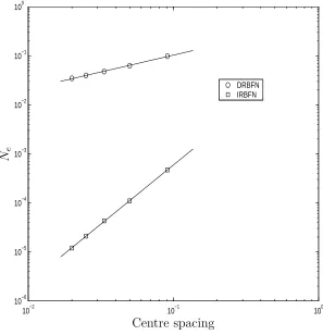
displayed in Figure 1, indicating that the IRBFN approach is superior to the DRBFN

in terms of accuracy and convergence rate. Highly accurate results and high rates

of convergence with “mesh” refinement are obtained with the present method. The

solution converges apparently as O(h3.4717_{) for IRBFN and O(h}1.3563_{) for DRBFN,}

where h is the centre spacing. At the finest density of 51×51, the error-norms are

2.0e−6 and 2.8e−3 for IRBFN and DRBFN respectively.

7.1.2 Poisson equation with both Dirichlet and Neumann conditions

In this example, the boundary conditions of the problem include both Dirichlet and

Neumann type. Consider the following PDE

∂2_u

∂x2 1

+ ∂

2_u

∂x2 2

on the square domain (0 ≤ x1 ≤ 1, 0 ≤ x2 ≤ 1) with the following boundary

conditions

u = exp(λx1+µx2), x2 = 0 and x2 = 1, (44)

∂u ∂x1

= λexp(λx1+µx2), x1 = 0 and x1 = 1. (45)

The exact solution to the above problem is

ue(x1, x2) = exp(λx1+µx2). (46)

Here, λ and µ are chosen to be 2 and 3, respectively. Special attention here is

given to the treatment for the Neumann condition ∂u/∂n. The present method

implements this type of boundary condition as follows. Along the left (x1 = 0)

and right (x1 = 1) sides of the domain, normal derivatives ∂u/∂n are given and

hence the task now is to express the boundary values of u there in terms of the

interior variable values. This can be achieved by solving the following subsystem of

equations

∂u(x(i)₎

∂x1

=

m

X

j=1

H[x1]H¯

−1

[x1]

[i,j]u

(j)_{, (47)}

where x(i) _={(x

1 = 0, x2),(x1 = 1, x2)}. Substitution of the results obtained from

(47) and the Dirichlet condition (44) into the final system of equations yields a

square system with the unknowns being only the interior variable values. Once the

final system of equations is solved, the numerical solution ualong two vertical sides

may be found from (47). Figure 2 displays results obtained by the DRBFN and

IRBFN approaches. The latter yields more accurate results and higher convergence

rates than the former. At the finest density of 51×51, the error-norms are 1.2e-5

for IRBFN and 3.4e-2 for DRBFN. The IRBFN solution converges apparently as

O(h2.4129_{) while the DRBFN solution apparently asO(h}0.6877_{), wherehis the centre}

7.2

Viscous flow

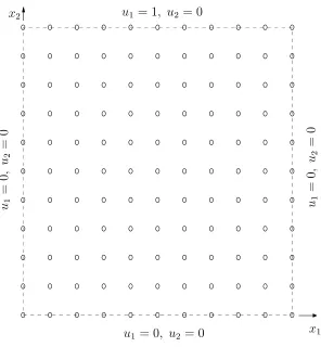
The benchmark problem of steady viscous flow in an unitary square cavity [22]

is simulated here to verify the present method. The fluid velocities on the left,

right and bottom walls are fixed at zero, while the top non-slip solid driving lid is

represented by a uniform non-zero velocity in the x1-direction along the top edge

(Figure 3). This problem is geometrically simple and has been used for decades as

a standard test problem to verify and validate numerical methods in computational

science and engineering. Ghia et al [23] provided a benchmark solution that is often

cited for comparison purposes.

It is noted that the moving lid introduces stress singularities at the two top corners.

At the upper corners, the velocity is discontinuous and the vorticity is unbounded.

The no-slip velocity conditions on the left, right and bottom walls ensure that

φ = 0, ∂φ

∂n = 0, (48)

while the uniform velocity of 1 along the top wall results in

φ = 0, ∂φ

∂n = 1, (49)

where n is the local direction normal to the wall. In the present work, the Poisson

equation for φ (28) and the vorticity transport equation (29) are solved

simultane-ously in a coupled manner.

In the case of Poisson equation ∇2u = s with a Neumann boundary condition

(∂u/∂n), it is known that the solution will exist only when the following

compati-bility condition is fulfilled

Z

∇u.ndΓ =

Z

where Γ denotes the boundary of the domain Ω. Even though equation (50) may

be fulfilled, the singular nature of the system of equations will present additional

complications [24]. Therefore, the direct employment of the Neumann condition

∂φ/∂n over all boundaries via a point collocation mechanism is not appropriate

here. Instead, it is used in generating a computational boundary condition for ω.

The process is as follows. In the first step, the vorticity in (28) can be simplified to

be

ω = −∂

2_φ ∂x2 1 −∂ 2_φ ∂x2 2 =−∂ 2_φ ∂x2 1

at the side walls, (51)

ω = −∂

2_φ ∂x2 1 −∂ 2_φ ∂x2 2 =−∂ 2_φ ∂x2 2

at the top and bottom walls, (52)

using the given boundary conditions. In the second step, they are written in terms

of first order derivatives ofφ

ω(i) = −∂

2_φ(i)

∂x2 1 = m X j=1

GH−_[x1_1]

[i,j]

∂φ ∂x1

(j)

at the side walls, (53)

ω(i) = −∂

2_φ(i)

∂x2 2 = m X j=1

GH−_[x1_2]

[i,j]

∂φ ∂x2

(j)

at the top and bottom walls,(54)

and the resulting expressions (53) and (54) are then simplified by taking into

consid-eration the Neumann condition for φ (∂φ/∂n). In the third step, the remainders of

the nodal first derivatives ofφ on the right-hand sides of (53) and (54) are expressed

in terms of the nodal stream function values, for example at the boundary point

x(i)_,

∂φ ∂x1

(i)

=

m

X

j=1

H[x1]H¯−_[x11]

[i,j]φ

(j)_{, (55)}

∂φ ∂x2

(i)

=

m

X

j=1

H[x2]H¯−_[x12]

[i,j]φ

(j)_{. (56)}

writ-ten in terms of the nodal values of φ. It is noted that in this process, the natural

boundary condition for the stream function is implemented in a precise manner.

The procedural flow chart involves the following steps

1. Input data such as geometries, boundary conditions, a Reynolds number and

data points including a set of centres and a set of collocation points,

2. Apply the IRBFN approach for the approximation of each variable and its

derivatives present in the relevant PDEs, which results in design matrices in

the network weight spaces. It is noted that these matrices are the same for all

variables,

3. Convert the multiple spaces of network weights into the single space of the

primary variable values,

4. Generate a computational Dirichlet boundary condition for ω corresponding

to the given Neumann boundary conditions,

5. Form the design matrix of the system, which involves only linear terms in the

governing equations (28) and (29), and then impose the Dirichlet conditions

for φ and ω. This matrix stays the same during the iteration process,

6. Initialize the stream function field and the vorticity field,

7. Compute the nonlinear convected vorticity terms, in which relevant derivative

functions are calculated in a straightforward manner using the network design

matrices obtained at step 3,

8. Formulate the trust region subproblem and then solve it for the search

direc-tion,

10. Check for convergence. If not yet converged, repeat from step 7,

11. Output the results.

Four sets of 31×31, 41×41, 51×51 and 61×61 uniformly distributed data points are

employed to study convergence. A range of Reynolds numbers {0,400,1000,2000

and 3200} is considered. For the current Reynolds number, the solution for the

previous value in the Reynolds number range is used as the initial solution and it

takes about 10 iterations to achieve a convergence by using the trust region method.

Another advantage of the trust region method over Picard-type iteration schemes

is that no relaxation scheme is required and hence it requires less parametric study.

Results obtained are in very good agreement with the benchmark solution of Ghia

[23], which was found by the multigrid finite difference method using a mesh size of

129×129. For example, velocity profiles along the vertical and horizontal centrelines

at some Reynolds numbers are displayed in Figures 4-6, where the IRBFN results

are very close to those of Ghia [23] and “mesh” convergence is achieved (i.e. greater

accuracy obtained with higher densities of data points used). Furthermore, in those

figures, streamline patterns for the flows are also presented, which agree well with

the benchmark solution.

Other important results are the properties of the primary vortex and the existence

of secondary vortices at the corners. It can be seen that all secondary vortices are

captured clearly, as shown in Figures 4-6. Several properties of the primary vortex

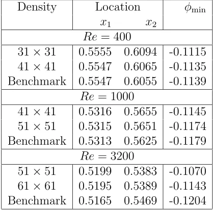
such as the location and the minimum value of the stream function are given in

the Table 1, showing that the present method yields a high degree of accuracy in

the primary vortex region. It can be also seen from the table that IRBFN results

are closer to the benchmark solution with an increase in data densities used (i.e.

8

Concluding remarks

This paper reports an efficient IRBFN method for solution of PDEs. The approach

differs from previous works in two aspects. The first one is that prior conversions

of the multiple spaces of network weights into the single space of nodal variable

values are introduced in order to form a square system of equations of smaller size,

resulting in a great improvement in the performance of the indirect RBFN method.

The second aspect is that the resulting nonlinear systems of equations are solved

by the trust region methods, which are more robust than the Newton-Raphson

type algorithms. The present method is truly meshless as no “finite element mesh”

is required for the purpose of interpolation and integration. Numerical examples

carried out in the paper show that accurate results and high rates of convergence with

refinement of spatial discretisation are achieved using relatively coarse discretizations

of the domain. This paper appears to be the first report achieving high Reynolds

number solutions by RBFNs. A disadvantage of the present method is that the

obtained system matrix is dense because the multiquadrics have non-local support

and how to overcome this disadvantage is a topic currently under investigation.

Acknowledgements

helpful comments. The computing facilities provided by The APAC National Facility

are gratefully acknowledged.

References

1. N. Mai-Duy and T. Tran-Cong, “Numerical solution of differential equations

using multiquadric radial basis function networks,” Neural Networks 14(2),

lishers, Albuquerque, 1998.

3. O. C. Zienkiewicz and R. L. Taylor, The Finite Element Method, McGraw-Hill,

London, 1991.

4. S. V. Patankar, Numerical Heat Transfer and Fluid Flow, McGraw-Hill, New

York, 1980.

5. P. K. Banerjee and R. Butterfield, Boundary Element Methods in Engineering

Science, McGraw-Hill, London, 1981.

6. C. A. Brebbia, J. C. F. Telles and L.C. Wrobel, Boundary Element Techniques

Theory and Applications in Engineering, Springer-Velag, Berlin, 1984.

7. D. Gottlieb and S. A. Orszag, Numerical Analysis of Spectral Methods: Theory

and Applications, SIAM, Philadelphia, 1977.

8. C. Bernardi and Y. Maday, “Spectral methods,” in Handbook of Numerical

Analysis, Vol. 5, P.G. Ciarlet and J.L. Lions (Editors), Elsevier Science, North

Holland, 1997.

9. C. Shu, Differential Quadrature and Its Application in Engineering,

Springer-Verlag, London, 2000.

10. E. J. Kansa, “Multiquadrics- A scattered data approximation scheme with

ap-plications to computational fluid-dynamics-II. Solutions to parabolic,

hyper-bolic and elliptic partial differential equations,” Computers and Mathematics

with Applications 19(8/9), 147 (1990).

11. J. Park and I. W. Sandberg, “Universal approximation using radial basis

func-tion networks,” Neural Computafunc-tion 3, 246 (1991).

12. J. Park and I. W. Sandberg, “Approximation and radial basis function

13. N. Mai-Duy and T. Tran-Cong, “Numerical solution of Navier-Stokes

equa-tions using multiquadric radial basis function networks,” International Journal

for Numerical Methods in Fluids 37, 65 (2001).

14. B. J. McCartin, “A model-trust region algorithm utilizing a quadratic

inter-polant,” Journal of Computational and Applied Mathematics 91, 249 (1998).

15. S. Haykin, Neural Networks: A Comprehensive Foundation, Prentice-Hall,

New Jersey, 1999.

16. R. Franke, “Scattered data interpolation: tests of some methods,”

Mathemat-ics of Computation 38(157), 181 (1982).

17. N. Mai-Duy and T. Tran-Cong, “Approximation of function and its

deriva-tives using radial basis function network methods,” Applied Mathematical

Modelling 27, 197 (2003).

18. S. N. Atluri and T. Zhu, “New concepts in meshless methods,” International

Journal for Numerical Methods in Engineering 47, 537 (2000).

19. G. F. Dargush and P. K. Banerjee, “A boundary element method for steady

in-compressible thermoviscous flow,” International Journal for Numerical

Meth-ods in Engineering 31, 1605 (1991).

20. J. J. More and D. C. Sorensen, “Computing a trust region step,” SIAM Journal

on Scientific and Statistical Computing 3, 553 (1983).

21. M. A. Branch , T. F. Coleman and Y. Li, “A subspace, interior and conjugate

gradient method for large-scale bound-constrained minimization problems,”

SIAM Journal on Scientific Computing 21, 1 (1999).

22. P.J. Roache, Verification and Validation in Computational Science and

23. U. Ghia, K. N. Ghia and C. T. Shin, “High-Re solutions for incompressible

flow using the Navier-Stokes equations and a multigrid method,” Journal of

Computational Physics 48, 387 (1982).

24. C. Pozrikidis, Introduction to Theoretical and Computational Fluid Dynamics,

Table 1: Lid-driven cavity flow: some properties of the primary vortex

Density Location φmin

x1 x2

Re= 400

31×31 0.5555 0.6094 -0.1115 41×41 0.5547 0.6065 -0.1135 Benchmark 0.5547 0.6055 -0.1139

Re= 1000

41×41 0.5316 0.5655 -0.1145 51×51 0.5315 0.5651 -0.1174 Benchmark 0.5313 0.5625 -0.1179

Re= 3200

10−2 10−1 100 10−6

10−5 10−4 10−3 10−2 10−1

DRBFN IRBFN

Centre spacing

Ne

Figure 1: Poisson equation, Dirichlet boundary condition: Solution accuracy and convergence rate by the DRBFN and IRBFN methods. The solutions converge apparently as O(h1.36_{) and O(h}3.47_{) for DRBFN and IRBFN respectively, where h}

10−2 10−1 100 10−6

10−5 10−4 10−3 10−2 10−1 100

DRBFN IRBFN

Centre spacing

Ne

Figure 2: Poisson equation, Dirichlet and Neumann boundary conditions: Solution accuracy and convergence rate by the DRBFN and IRBFN methods. The solutions converge apparently as O(h0.69_{) and O(h}2.41_{) for DRBFN and IRBFN respectively,}

x1

x2

u1

=

0

,

u2

=

0

u1

=

0

,

u2

=

0

u1 = 0, u2 = 0

u1 = 1, u2 = 0

−0.40 −0.2 0 0.2 0.4 0.6 0.8 1 0.1

0.2 0.3 0.4 0.5 0.6 0.7 0.8 0.9 1

Benchmark

31× 31

41× 41

a) u1 on the vertical centreline

u1

x2

0 0.1 0.2 0.3 0.4 0.5 0.6 0.7 0.8 0.9 1

−0.5 −0.4 −0.3 −0.2 −0.1 0 0.1 0.2 0.3 0.4

Benchmark

31× 31

41× 41

b)u2 on the horizontal centreline

x1

u2

c) Streamline pattern

−0.40 −0.2 0 0.2 0.4 0.6 0.8 1 0.1

0.2 0.3 0.4 0.5 0.6 0.7 0.8 0.9 1

Benchmark

41× 41

51× 51

a) u1 on the vertical centreline

u1

x2

0 0.1 0.2 0.3 0.4 0.5 0.6 0.7 0.8 0.9 1

−0.6 −0.5 −0.4 −0.3 −0.2 −0.1 0 0.1 0.2 0.3 0.4

Benchmark

41× 41

51× 51

b)u2 on the horizontal centreline

x1

u2

c) Streamline pattern

−0.50 0 0.5 1 0.1

0.2 0.3 0.4 0.5 0.6 0.7 0.8 0.9 1

Benchmark

51× 51

61× 61

a) u1 on the vertical centreline

u1

x2

0 0.1 0.2 0.3 0.4 0.5 0.6 0.7 0.8 0.9 1

−0.8 −0.6 −0.4 −0.2 0 0.2 0.4 0.6

Benchmark

51× 51

61× 61

b)u2 on the horizontal centreline

x1

u2

c) Streamline pattern