A study on the biology of Osangularia cf. venusta (Brady): an epiphytic foraminifera on the intertidal seagrass Halodule uninervis in Shelly Bay, Townsville, North Queensland

Full text

(1)ResearchOnline@JCU. This file is part of the following reference:. Ludvianto, Bayu (1992) A study on the biology of Osangularia cf. venusta (Brady): an epiphytic foraminifera on the intertidal seagrass Halodule uninervis in Shelly Bay, Townsville, North Queensland. PhD thesis, James Cook University of North Queensland.. Access to this file is available from:. http://researchonline.jcu.edu.au/33779/ If you believe that this work constitutes a copyright infringement, please contact ResearchOnline@jcu.edu.au and quote http://researchonline.jcu.edu.au/33779/.

(2) A study on the biology of Osangularia cf. venusta (Brady): an epiphytic foraminifera on the intertidal seagrass Halodule uninervis in Shelly Bay, Townsville, North Queensland.. Thesis submitted by Bayu LUDVIANTO BSc, Sarjana Biologi cum laude (Gadjah Mada University, Indonesia) in August 1992. for the degree of Doctor of Philosophy in the Department of Marine Biology at James Cook University of North Queensland.

(3) STATEMENT OF ACCESS. I, the undersigned, the author of this thesis, understand that James Cook University of North Queensland will make it available for use within the University Library and, by microfilm or other photographic means, allow access to users in other approved libraries. All users consulting this thesis will have to sign the following statement : "In consulting this thesis I agree not to copy or closely paraphase it in whole or in part without the written consent of the author; and to make proper written acknowledgement for my assistance which I have obtained from it." Beyond this, I do not wish to place any restriction on acces to this thesis.. 25. 1. •. oe.. VO9.

(4) ABSTRACT. A study on the biology of an epiphytic foraminifera. (Osangularia cf. venusta) has been conducted in the intertidal zone at Shelly Bay near Townsville, Australia, during the period of 1988 to 1990. The aims of the study were 1) to understand the general biology of O. cf. venusta, 2) to investigate the temporal patterns of O. cf. venusta distribution and its relationship with the substratum (seagrass blades), 3) to obtain information on the population' dynamics of O. cf. venusta including growth rate, recolonization, and migration. Sampling was carried out during low tide (< 0.5 metres), over three different time intervals : 1) monthly, 2) fortnightly, and 3) daily. Samples were fixed by using 70 % ethanol as soon as the field works were completed. O. cf. venusta specimens were collected by detaching them from the seagrass blades under a stereo microscope. Detailed observations of the specimen was made by means of a stereo microscope and a scanning electron microscope. Locomotion was observed by video recording the movements of O. cf. venusta individuals on the Halodule uninervis blades. The study shows that individuals dislodging by physical and biological forces, may influence the population dynamics of O. cf.venusta especially the. ii.

(5) "age" distribution. These factors were also suspected to affect the temporal abundance, density and the proportion of microspheric and megalospheric individuals in the population. Other factors such as the condition of the seagrass, its abundance and blade area are also strongly believed to affect the temporal abundance of O. cf. venusta. Generally, left coiled individuals dominated the population during the study period. This coiling direction preference, however, could not be correlated to the temperature variations of the surrounding environment. "Twinned" specimens were observed in the O. cf. venusta population during the study period. The study shows that the "twinned" phenomenon in O. cf. venusta was probably initiated by the creation of a second aperture whilst the juvenile had only one chamber. The juvenile, then developed two rows of later chambers based on the two apertures. The present study also reveals that 0.cf.venusta maintained its existence in the harsh intertidal environment by 1) reinforcing the test, 2) producing a large number of juveniles, 3) clinging on the blades of the intertidal seagrass Halodule uninervis, and 4) rapidly colonizing and recolonizing the "empty" seagrass blades.. iii.

(6) LIST OF CONTENTS. List of figures. vii. List of tables. xii. Declaration. xiv. Aknowledgements. xv. Chapter I 1.1. General Introduction 1.2. The history of the taxonomic position of Osangularia cf.venusta. 10. Chapter II 2.1. Site description 2.2. Materials and methods 2.2.1 General field methods 2.2.2 General laboratory methods • • • •. 14 14 16 16 17. 1 1. Chapter III Temporal distribution of Osangularia cf.venusta and its relationship with the seagrass as a substratum. . . 18 3.1. Introduction 18 3.2. Materials and methods 19 3.2.1. Field work: 19 3.2.1.1. Seagrass preference. . . 19 3.2.1.2. Temporal distribution of O.cf.venusta and its relation to the area of seagrass blades (experiment 1) 20 3.2.1.3. Temporal distribution of O.cf.venusta and its relation to the abundance of the seagrass blades (experiment 2) 25 3.2.2. Laboratory work• 26 3.2.2.1. Experiment 1 26 3.2.2.2. Experiment 2 27 3.3. Analysis of data 27 3.4. Results 28 3.4.1. Seagrass preference of 0.cf. venusta at Shelly bay, Pallarenda 28 3.4.2. Monthly temporal density and abundance and its relationship with the area of the blades. 31 3.4.3. Monthly temporal O.cf.venusta abundance in relation to the temporal abundance of the blades. 38 3.5. Discussion 39 Chapter IV Morphology of Osangularia cf.venusta :its abnormality and uses in the temporal study. iv. 48.

(7) 4.1. General morphology of Q.cf.venusta. . 4.1.1. Introduction 4.1.2. Material and methods 4.1.3. Results 4.1.3.1. Megalospheric and microspheric morphology. • • 4.1.3.2. Mature microspheric morphology 4.1.4. Discussion 4.2. Test abnormality in Q.cf.venusta • • 4.2.1. Introduction. 4.2.2. Results 4.2.3. Discussion 4.3. Coiling direction as one of the morphological characteristics in Q.cf.venusta 4.3.1.Introduction 4.3.2. Materials and methods 4.3.3. Results 4.3.3.1. Monthly study 4.3.3.2. Fortnightly study. . . . 4.3.3.3. Relationship between the proportion of sinistrally coiled individuals with temperatures 4.3.4. Discussion 4.4. Microspheric and megalospheric generations: their occurence and temporal patterns in the population 4.4.1.Introduction 4.4.2. Materials and methods 4.4.3. Results 4.4.4. Discussion.. Chapter V Population study 5.1. Population dynamics 5.1.1. Introduction 5.1.2. Materials and methods 5.1.3. Results 5.1.4. Discussion 5.2. Recolonization study 5.2.1. Introduction 5.2.2. Materials and methods 5.2.2.1. Field work 5.2.2.2. Laboratory work 5.2.3. Results 5.2.4 Discussion 5.3. The role of movements and migration in shaping the population of Q.cf.venusta on the blades of Halodule uninervis 5.3.1.Introduction 5.3.2. Materials and Methods 5.3.2.1. Field investigation. • • • 5.3.2.2. Laboratory work. 5.3.2.3. Data analysis.. 48 48 52 53 53. 60 64 68 68 70 72 76 76 79 85 85 85. 91 91 101 101 104 105 106 113 113 113 117 119 136 142 142 145 145 147 147 150 156 156 158 158 160 161.

(8) 5.3.2.4. Laboratory investigations. 5.3.3. Results 5.3.3.1. Field investigations. . . 5.3.3.2. Laboratory video investigation 5.3.4. Discussion.. 162 166 166 173 174. Chapter VI Concluding Discussion.. 178. References. 185. vi.

(9) LIST OF FIGURES. Figure 1: Study site at Shelly Bay, Townsville, North Queensland Figure 2: Study area and sampling site in Shelly Bay Figure 3: Sampling design used for studying the temporal mean abundance of Q.cf.venusta during October 1988 to March 1989 Figure 4: Sampling design for studying the temporal abundance of 0.cf,venusta during April 1989 to September 1989. Figure 5: Quadrants at each location of Experiment 1, period 2 (April 1989 to September 1989). . Figure 6 a, b, c: Monthly Q.cf.venusta mean abundance at location 1, 3, and 5 Figure 7 a, b, and c: Monthly 0.cf.venusta density at location 1, 3, and 5 Figure 8 a, b, and c: Monthly mean area of seagrass blade at location 1, 3, and 5 Figure 9: Number of 0.cf.venusta vs number of seagrass blades per plot in experiment 2 during October 1988 to March 1989 Figure 10: Number of Q.cf.venusta vs number of seagrass blades per plot in experiment 2 during April 1989 to September 1989 Figure 11: Osangularia cf.venusta, megalospheric specimen, dorsal view Figure 12: Osangularia cf.venusta, microspheric specimen, ventral view Figure 13: Apertural view Figure 14: Two different types of pustules . . . Figure 15: Long, sharp pointed pustules near the umbilical plug. Figure 16: Short, rounded pustules near periphery at the ventral side Figure 17: Short, rounded pustules at the dorsal side Figure 18: Umbilical side. Figure 19: Detail of the umbilical plug. Figure 20: Pores viewed from the internal chamber wall Figure 21: Pores viewed from the internal chamber wall Figure 22: Cross section of the ultimate chamber wall Figure 23: Cross section of the ultimate chamber wall. Figure 24: Cross section of the penultimate chamber wall. Figure 25: Apertural view of Q.cf.venusta showing the shape and position of the main aperture Figure 26: Brood chamber aperture vii. 15 21 22 23 24 35 36 37 44 44. 55 55 55 55 55 55 55 55 55 55 56 56 56 56 56 56.

(10) Figure 27: Brood chamber aperture Figure 28: Brood chamber aperture Figure 29: Broken ultimate chamber, showing the "china wall-like" plate Figure 30: Detail of the " china wall-like " plate Figure 31: Internal structure of the aperture, in relation to the "china wall-like" plate. . . . Figure 32: The "china wall-like" plate at the third chamber before the ultimate chamber Figure 33: Broken ultimate chamber showing the inner lamellae and the outer lamella in relation to the whole chamber structure. . • • Figure 34: The inner lamellae Figure 35: Apertural face of the penultimate chamber Figure 36: Mature microspheric with brood chambers Figure 37 and 38: Mature microspherics Figure 39: Mature microspheric with one brood chamber Figure 40: Mature microspheric specimen with two brood chambers Figure 41: Broken brood chamber showing the position of the intercameral foramen of the base chamber and the "china wall-like" plate. Figure 42: Detail position of the "china wall-like" plate in relation to the intercameral foramen of the base chamber Figure 43: Broken brood chamber showing the relationship between the "china wall-like" plate with the internal intercameral foramen. Figure 44: Detail of the internal chamber wall of the brood chamber Figure 45: Mature microspheric with juveniles. . Figure 46: Two live mature microspheric individuals with the juveniles that had just been released and spread along the blade Figure 47: Remains of the brood chambers Figure 48: Broken ultimate chamber showing the origin of the aperture lip. Figure 49: Cross section of the base chamber of the mature microspheric specimen. Figure 50: Enlargement of Figure 48, showing the detailed of the connection between the two lamina Figure 51: Twinned specimen Figure 52: The intercameral foramen of the penultimate chamber of the twinned specimen. Figure 53: Equatorial view of "twinned" specimens, showing the complete joining of the early chamber Figure 54: Apertural view, showing partial joining of the early chambers Figure 55: Detail structure of the external chamber wall and aperture. viii. 56 56 56 56 59 59 59 59 59 59 59 59 59 63 63 63 63 63 63 63 63 63 63 71 71 71 71 73.

(11) Figure 56: Early development of "twinned" individual of O.cf.venusta Figure 57: Monthly percentage of left coiled megalospheric and microspheric individuals per blade Figure 58: Monthly percentage of right coiled megalospheric and microspheric individual per blade Figure 59: Monthly percentage of left and right coiled 0.cf.venusta per blade Figure 60: Fortnightly percentage of left and right coiled 0.cf.venusta per blade at site 1. . . . Figure 61: Fortnightly percentage of left and right coiled 0.cf.venusta per blade at site 2. . . Figure 62: Monthly temperature in Shelly Bay, during April 1989 to September 1989 Figure 63: Fortnightly immersed sediment temperature in relation to the percentage of left coiled individual per blade at site 1. . Figure 64: Fortnightly immersed sediment temperature in relation to the percentage of left coiled individuals per blade at site 2. . Figure 65: Monthly percentage of megalospheric and microspheric individuals per blade during October 1988 to September 1989. Figure 66: Fortnightly percentage of microspheric individuals per blade at Site 1 Figure 67: Fortnightly percentage of microspheric individuals per blade at Site 2 Figure 68: Relationship between the number of chambers and size in microspheric and megalospheric specimens Figure 69: Monthly number of chambers of megalospheric individuals Figure 70: Monthly mean number of chambers of specimens collected from Experiment 1 of the temporal distribution study Figure 71: Fortnightly number of chambers of megalospheric specimens collected from Experiment 1, Site 1 of the recolonization study Figure 72: Fortnightly number of chambers of megalospheric specimens collected from Experiment 2, Site 1 of the recolonization study Figure 73: Fortnightly number of chambers of megalospheric specimens collected from Experiment 3, Site 1 of the recolonization study Figure 74: Fortnightly number of chambers of megalospheric specimens collected from Experiment 1, Site 2 of the recolonization study Figure 75: Fortnightly number of chambers of megalospheric specimens collected from. ix. 75 81 81 81 82 83 92 94 94 109 109 109 120 121 123. 124. 125. 126. 127.

(12) Experiment 2, Site 2 of the recolonization study 128 Figure 76: Fortnightly number of chambers of megalospheric specimens collected from Experiment 3, Site 2 of the recolonization study 129 Figure 77: Trends of the mean number of chambers of left coiled megalospheric individuals collected from Site 1 of the recolonization study 131 Figure 78: Trends of the mean number of chambers of right coiled megalospheric individuals collected from Site 1 of the recolonization study 132 Figure 79: Trends of the mean number of chambers of left coiled megalospheric individuals collected from Site 2 of the recolonization study 133 Figure 80: Trends of the mean number of chambers of right coiled megalospheric individuals collected from Site 2 of the recolonization study 134 Figure 81: Percentages of microspheric mature specimens collected from Experiment 1 and 2 of the temporal distribution study (October 1988 - September 1989). 135 Figure 82: Percentages of microspheric mature specimens in relation to the number of 0.cf.venusta per plot in Experiment 2 of the temporal distribution study 135 Figure 83: Percentages of microspheric and megalospheric specimens in Experiment 1 of the temporal distribution study 135 Figure 84: Mean number of individuals per blade of the samples collected from Experiment 1 of the temporal distribution study (April 1989 to September 1989) 144 Figure 85: Sampling design for the recolonization study. ' 146 Figure 86: Mean number of individuals per blade in Site 1 during 60 days study period. 148 Figure 87: Mean number of individuals per blade in Site 2 during 60 days study period. 148 Figure 88: Temporal mean number of individuals per blade in Site 1 149 Figure 89: Temporal mean number of individuals per blade in Site 2 149 Figure 90: Field experimental design for studying the effect of blade conditions and space barrier on the epiphytic foraminiferal population. 159 Figure 91: Sampling design for studying the effect of blade conditions and space barrier on the number of 0.cf.venusta in August 1990 163. x.

(13) Figure 92: Daily number of individuals of 0.cf.venusta per six "natural" seagrass blades in August 1990. Figure 93: Daily number of individuals of 0.cf.venusta per six "cleaned" seagrass blades in August 1990. Figure 94: Daily number of individuals of 0.cf.venusta per six "natural" seagrass blades in September 1990 Figure 95: Daily number of individuals of 0.cf.venusta per six "cleaned" seagrass blades in September 1990 Figure 96: Daily number of individuals of 0.cf.venusta per one gram of sediment beneath the "natural" seagrass blades condition, in August 1990 Figure 97: Daily number of live 0.cf.venusta per one gram of sediment beneath the "natural" seagrass blades condition, in August 1990. . Figure 98: Daily number of individuals of 0.cf.venusta per one gram of sediment beneath the "cleaned" seagrass blades condition, in August 1990 Figure 99: Daily number of live individuals of 0.cf.venusta per one gram of sediment beneath the "cleaned" seagrass blades condition, in August 1990. xi. 167 167 16 8 .. 168. 169 169. 170. 170.

(14) LIST OF TABLES Table 1: Result of the ANOVA on the 0.cf.venusta mean abundance between the two species of seagrass (Halophila ovalis and Halodule uninervis) found in Shelly Bay. Table 2: Result of the ANOVA on the 0.cf.venusta mean abundance between the two species of seagrass (Halophila ovalis and Halodule uninervis) found in Shelly Beach. Table 3: Result of the ANOVA on the monthly (October 1988 to March 1989) mean abundance. Table 4: Result of the ANOVA on the monthly 0.cf.venusta mean abundance during the period of April 1989 to September 1989 Table 5: Summary of the simple correlation coefficient between the 0.cf.venusta abundance and the area of blades Table 6: Result of the ANOVA on regression between the number of 0.cf.venusta and the number of blades per 18 plots (1 plot = 78.53 cm 2 ) during the period of October 1988 to March 1989 . . . Table 7: Result of the ANOVA on regression between the number of 0.cf.venusta and the number of blades per 36 plots (1 plot = 78.53 cm 2 ) during the period of April to September 1989 . . . Table 8: Result of the ANOVA on the monthly mean blades abundance during the period of April 1989 to September 1989 Table 9: Result of the Anova on the temporal proportion of left coiled individuals in the population during April to September 1989. . . Table 10: Result of the ANOVA testing the effect of Sites, Starting dates of experiment and Periods of sampling on the proportion of left coiled individuals. Table 11: Polynomial Contrast for testing the trends of the proportion of left coiled individuals over four periods of sampling . Table 12: Summary of the ANOVA testing the difference of the left coiled proportion among Periods at different Starting dates and Sites. Table 13: Summary of the simple regression between the percentage of left (% left) or right (% right) and the monthly temperature. Table 14: Summary of the regression analysis on the relationship between the proportion of left coiled direction (% left) and immersed sediment temperature (T). Table 15: Number of individuals of each generation per eight and sixteen blades of Halodule uninervis Table 16: Number of individuals of each generation in six blades of Halodule uninervis. • • • •. xii. 29. 30 33. 34 40. 41. 42 43 87. 88 89 90 93. 93. 107. 108.

(15) Table 17: The percentages of micropsheric mature form in relation to the total specimens in six seagrass blades at Site 1 Table 18: The percentages of micropsheric mature form in relation to the total specimens in six seagrass blades at Site 2 Table 19: Result of the ANOVA testing the effect of Sites, Starting Dates of experiement and Periods of sampling on the number of individual per blade Table 20: Polynomial Contrast for testing the trend of mean number of individuals during the Periods of sampling Table 21: Summary of the Anova testing the different among Periods at different experiment Starting dates Table 22: Result of the ANOVA on the daily 0.cf.venusta mean abundance in August 1990. Table 23: Result of the ANOVA on the daily 0.cf.venusta mean abundance in September 1990. Table 24: Result of polynomial contrast of mean abundance of 0.cf.venusta by Day in August 1990. Table 25: Result of polynomial contrast of mean abundance of 0.cf.venusta by Day in September 1990.. 137 137. 152 153 154 164 165 172 172.

(16) DECLARATION. I declare that this thesis is my own work and has not been submitted in any form for another degree or diploma at any university or other institution of tertiary education. Information derived from the published or unpublished work of others has been acknowledged in the text and a list of references is given.. B. L. anto .August 1992.. xi v.

(17) Acknowledgements. In completing this project, I would like to express my special thanks to my supervisor Dr.J.D.Collins, for his support and advice during the preparation of the project and the thesis. I also would like to thank IDP and AIDAB for granting me the scholarship and financially supporting my project: and Prof. H. Choat for his support in the Department of Marine Biology at James Cook University. My thanks are also extended to the following people: Tri Eddy Kuriandewa, Otty, Dede Hartono, Budi Hendrarto, Dwatmadji, Maureen Yap, Temakei Tebano, Suzanne Mingoa, Craig Blount, Ron Wakely and, Gozali Moekti for their invaluable assistance in the field and sacrificing their precious sleeping time to be a "night wanderer" during the period of October to March 1988/1989 and also 1989/1990. I am also indebted to Mr Glen De'ath, Dr. Bruce Mapstone, Dr. Garry Russ and Dr. Hugh Sweatman for their expert advice with sampling designs and statistical analysis. I can not thank enough Professor Dr. Lukas Hottinger and Dr. Iradj Yassini for their advice in establishing the taxonomic position of Osangularia cf.venusta. I wish to thank Leigh Winsor and Zoli Florian for their guidence in Histology and Microscopy. I would like to thank A/Prof. C.G. Alexander for his generosity in allowing me to use his video recording equipment, and Jim Darley for his expert advice in.

(18) scanning electron microscopy. Phil and Kim Osmond, Don Ross, Gordon Bailey, Don Booth, Anita Murray, Alan Wignall, Claudia McGrath, John Peters, Vince Pullella and Ann Sharp also warrant special acknowledgements for their advice, help and friendship. My very special thanks are extended to my dearest friends Giliane Brodie, Nina Morissette and Rob McGill for their support and encouragement during the preparation of this thesis. I would like also to thank Joy Walterson, Linda and Graham Wakely, for their welcoming hands and understanding during my time in Australia. Finally, I must thank my wife Sita for her warm support and understanding, especially during the hard times in dealing with this project.. xvi.

(19) 1. Chapter I. 1.1. General Introduction. Foraminifera are single celled organisms that mostly secrete calcareous shells and live in the marine habitat and in the nineteenth century amazingly brought together a chemist, Brady; a grocer, Wright; a surgeon, Flint; and a post office official, Earland, into one "interest" of study. These pioneer workers in foraminifera, were fascinated by the beauty of foraminiferal tests and their usefulness in the geologic field (Haynes, 1981). The range of size of foraminifera (between 0.10 mm to more than 5 mm) allow them to be used as "index fossils" in oil exploration and other subsurface studies (Haynes, 1981). Of even greater value is their wide distribution in most sedimentary rock particularly in clay, silt , fine sand, coarse sand and limestone. Besides their use in the geological studies, more recently, foraminifera have been used to investigate water mass movement (Boltovskoy and Wright, 1976), marine pollution (Bates and Spencer, 1979), marine environmental stress (Bock, 1976) and sediment production (Muller, 1976). The studies of foraminiferal biology can be separated into two main topics i.e. 1) detailed investigations of the species and, 2) studies on the.

(20) 2. relationship between species or group of species and the surrounding environment. Detailed studies on the foraminiferal species have included investigations on fine structure of foraminiferal protoplasm (Lee et al., 1965; Marzalek, 1969; Anderson and Be, 1978; Alexander and Banner, 1984), test morphology and test abnormality (Hottinger, Halicz and Reiss, 1991; Hansen and Reiss, 1972; Hottinger, Halicz and Reiss, 1991; Bolotovskoy, 1982; Boltovskoy, Scott and Medioli, 1991; Akturk, 1976; Be and Spero, 1981), growth (Bradshaw, 1957; Murray, 1983; Hallock et al., 1986; Bijma et al., 1990), life cycle, reproduction and alternation of generations (Lutze and Wefer, 1980; Rottger, Kruger and de Rijk, 1990; Angell, 1990; Rottger, Fladung, Schmaljohann, Splinder and Zacharias, 1986; Goldstein, 1988; Grell, 1988; Kloos, 1984) and, behaviour (Kitazato, 1988 and Wienberg, 1991). The studies on the relationship between foraminifera and their surrounding environments are spatial and temporal distribution (Boltovskoy and Lena, 1969; Boltovskoy and Wright, 1976; Coleman, 1979; Michie, 1982 and 1987; Moodley, 1990; Jennings and Nelson, 1992; Sautter and Thunell, 1989 , migration (Walker, 1976; Bock, 1969),.

(21) 3. population dynamics and sediments production (Murray, 1967 and 1983; Reynolds and Thunnell, 1986; Berger, 1971; Muller, 1974; Hallock et al., 1986; Erskian and Lipps, 1987), association (Dobson and Haynes, 1973; Haward and Haynes, 1976; Zumwalt and Delaca, 1980; Bock, 1967 and 1969; Brasier, 1975; Severin, 1983 and 1987) and, colonization and recolonization (Ellison and Peck, 1983; Buzas et al., 1989; Buzas, 1978; Finger and Lipps, 1981). Living foraminifera can be observed in tide pools, estuaries and lagoons, intertidal zones, and inner shelf zones to the abyssal plains (Boersma, 1978; Brasier, 1980; Murray, 1973). Foraminifera in the intertidal zone, have been extensively studied by many workers such as Reiter (1959), Cooper (1961), Boltovskoy (1963 and 1966) and Boltovskoy and Lena (1970). Because of the unique conditions of the intertidal zone (subject to twicedaily subaerial exposure, diurnal temperature changes, evaporation, rainfall and alteration of salinity), species of foraminifera that occupy this area are very well adapted to life in extreme conditions (Murray, 1973; Boltovskoy and Wright, 1976). Species may have flat tests, living attached to the substratum. (Rotorbinella, Discorbis, Trochammina, Rotorbinella lomaensis (Bandy), R. turbinata (Cushman and Valentine), Discorbis monicana, Zalesny and Trochammina pacifica.

(22) 4 (Cushman), or have thick and strong walls (Elphidium crispum, Quinqueloculina seminulum, Rotalia becarii) to survive living in the intertidal zone (Reiter, 1959; Boltovskoy and Wright, 1976). According to Boltovskoy and Wright (1976) it is important to differentiate the living from the dead specimens when dealing with the foraminifera in the intertidal zone. This is because of the extensive sediment movement in this region that can cause faunal mixed up. Many studies have shown that only a small percentage of the species found in the intertidal zones can be considered as living specimens. Reiter (1959) for instance reported only 17 were found living from 129 species observed in Santa Monica Bay, California. He also highlighted the seasonal variations in the number of individuals and species of foraminifera in Santa Monica Bay during his seven year study period. Cooper (1961) examined samples from San Diego, California northward to Colombia River, Oregon and stated that from the 120 species found only 64 species had live specimens. In Puerto Deseado, Argentina Boltovskoy (1963) and Boltovskoy and Lena (1966;1970) discovered that only 50 % of 130 species had live specimens. Unfortunately, the method of differentiating the live and dead foraminifera found in the sediment is still the subject of debate. The most common method used to differentiate live foraminifera from dead is by the.

(23) 5. use of the vital stain method that was introduced by Walton (1952) and the Sudan Black B fat staining method of Walker et all. (1974). These methods have proven unsatisfactory, because both the living and dead foraminifera are often stained together. This appears to be caused by the non-living protoplasm remaining inside the dead test for some period (Bernhard, 1988). Recently, De Laca (1986) introduced ATP analyses in order to differentiate the living foraminiferal from the dead population, however this method is both expensive and time consuming. Boltovskoy and Wright (1976) stated that foraminiferal distribution is controlled by several ecological factors such as depth, temperature, salinity, nutrition, substratum, pH, light intensity, turbidity, organic content of substratum and the concentration of oxygen and calcium carbonate in the seawater. Substratum, as one of the ecological factors, has been defined by foraminiferal investigators as the sediment and/or other organisms on the sediment (including weed and grass) where benthic foraminifera live. In the interest of ecology this definition should be refined so that foraminifera living on sediment are distinguished clearly from foraminifera living epiphytically or epizoically, thus the effect of substratum on the organisms would be more precise. Seagrass such as : Posidonia, Cymodocea, Halophila, Halodule, Enhalus and, Thalassia have been reported to.

(24) 6. be the substratum occupied by many species of foraminifera (Martin and Wright, 1988; Bock, 1969; Severin, 1987; Faber, 1991; Davies, 1970). Epiphytic foraminifera usually attach themselves to the substratum by means of an organic matrix, as shown by Delaca and Lipps (1972) in Rosalina globularis. After death the attachment materials decompose and the test falls down to the sediments beneath the seagrass. Thus, only live specimens will be found attached to the seagrass blades. Because, 1) the problem with differentiating between the live and dead foraminifera and 2) ease with which live foraminifera living epiphytically can be distinguished, it is concluded that biological and ecological studies of the intertidal foraminifera are more relevant to be undertaken on the epiphytic species. Bock (1967) pioneered the study of epiphytic foraminifera living in seagrass beds. He concluded that seagrass (Thalassia testudinum) provides a habitat and means of dispersal for several foraminifera such as. Archaias anqulatus, Articulina mucronata, Fursenkoina complanata, Miliolina circularis, M. labiosa, Nubecularia cf N.lucifaga, Rosalina floridana, Sorites marginalis and Triloculina bermudezi in the Florida Keys. Davies (1970) in his study at Eastern Shark Bay, Western Australia found that Peneroplis planatus,. Marginipora vertebralis, Vertebralina striata, Nuberculina sp, Spirilina sp, Patellina §p, Discorbis.

(25) 7. dimidiatus all live on segrasses (including Posidonia. and Cymodocea). He defined these organisms as epibiont foraminifera and suggested that these foraminifera contribute a significant amount of skeletal material to the carbonate sediment banks in this area. In his research, Brasier (1975a) discovered that the diversity of foraminiferal tests is higher in the seagrass areas of Alligator Reef, South Jamaica. Murray (1970, in Brasier, 1975a) stated that in Abu Dhabi Lagoon, the diversity and standing crop of foraminifera was improved by the colonization of seagrass. In a study of the importance of substratum in determining the character of foraminiferal biofacies in the lagoon of Barbuda, West Indies, Brasier (1975) concluded that the phytal substratum seems to control the distribution and standing crop of foraminifera. The word "phytal" was coined by Brasier to signify that the substrata where foraminifera lived consisted of weed and grass. However, he even included hard substrata derived from molluscs and corals into his "phytal" definition! He also found that the habitats with phytal substrata promoted an increase of foraminiferal standing crop. Although he listed foraminifera found on phytal surfaces, he did not, however, make a clear distinction between which "phytal" substrata supported which foraminifera, nor did he distinguished between weed and grass..

(26) 8 Blanc-Vernet (1969 in Brasier, 1975) and Davies (1970) stated that Peneroplis planatus has a parallel distribution and is associated with Cymodocea, and that other foraminifera such as Sorites marginalis and Amphisorus hemprichii seems to have a parallel. distribution with Thallassia beds (which also included Halophila, Syringodium and Halodule).. Based on the above work and other research, Brasier (1975) used foraminifera to interpret the paleodistribution of a seagrass community. In this study he tried to match the appearance of certain foraminifera and seagrass species in time and space, and he concluded that "the distribution of recent and fossil seagrass are similar to the distribution of Recent and fossil seagrass-dwelling foraminifera". Unfortunately, most of the studies on epiphytic foraminifera were either carried out in deeper water or undertaken only for the purpose of identifying the number of species. The study of the biology and ecology of a specific epiphytic foraminifera in the intertidal zone is still wanting. Quantitative evidence on the biology and ecology of epiphytic foraminifera and their relationships with seagrass as a substratum thus needs to be gathered. The pilot study that was conducted in early 1988 in the intertidal zone at Shelly Bay near Townsville, showed that the seagrass (Halodule uninervis) which occupied most of this area was inhabited by a species of.

(27) 9 foraminifera called Osangularia cf.venusta (Brady). The published information on 0.cf.venusta and its relationship with the substratum (H.uninervis) is very limited. Coleman (1979) reported that specimens of Pararotalia venusta (which might be more correctly. called Osangularia cf.venusta) were collected at depths ranging from 3 to 10 fathoms in Bowling Green Bay, North Queensland. Michie (1982 and 1987) collected Pararotalia venusta from Port Darwin, which was associated with. calcareous sands and coral reef. He also stated that 10 % of his foraminiferal assemblages from the outer harbour region and off Lee Point, were comprised of P.venusta. These two reports, however, were based on. sediment samples in which the method of differentiating the live and dead foraminifera still needs to be improved, and thus the place where P.venusta was found, is not neccessarily the actual habitat of this species. There are at least three major advantages in using an epiphytic foraminifera in order to study the biology of intertidal foraminifera 1) the problems of reworked specimens is avoided, 2) there is no need for an extra step in the work to differentiate the living specimens from the their dead counterparts and 3) the specimens are always available in large numbers for the whole year, so statistically valid analyses can be performed. During the study time, samples were taken over three different time intervals i.e : monthly,.

(28) 10. fortnightly and daily. Seagrass blades were sampled during low tides that exposed the seagrass beds (<0.5m). The present study was set up to investigate 1) the general biology of the intertidal epiphytic foraminifera 2) the patterns of the temporal distribution of 0.cf.venusta and its relationship with the substratum. (seagrass blades), 3) the population dynamics of 0.cf.venusta including growth rate, recolonization and. migration.. 1.2. The history of the taxonomic position of Osangularia cf.venusta .. Specimens which are morphologically identical with the specimens collected by the author from Shelly Bay during the present study, were first recorded by Brady (1884) as Rotalia venusta, n. sp. from South Pacific Stations. Brady's specimens mostly came from the islands south of Papua from depth of 3 to 11 fathoms. He also obtained specimens from the west coast of Patagonia off Middle Island, at the depth of 345 fathoms. These specimens which were about 0.75 mm diameter, had sublenticular tests, in which the dorsal face was nearly flat and the ventral face was convex. The external surface of the test was granular or rugose. The sutures were limbate on the dorsal face and deeply excavated on the ventral. The last whorl consisted of eight chambers.

(29) 11. and the aperture was an elongate fissure on the inner side of the final segment. The most noticeble difference between the morphology of the specimens collected from Shelly Bay and Brady's (1884) descriptions, is on the characteristics of the aperture, especially the shape and the lack of apertural lip in Brady's specimens. The specimens collected from Shelly Bay have an aerial, arched, slit-like aperture that is characterised by the presence of a murus reflectus and an apertural lip. Heron-Allen and Earland (1914 and 1915) discovered that Rotalia venusta was the most abundant and typical species in the Kerimba archipelago (Portuguese East Africa). This archipelago was characterised by extensive sandy beaches, stretches of rock-bound coast and mangrove swamps. The main islands are of coral formations and surounded by fringing and barrier reef.. R.venusta was abundant in most of the sampling stations (depth 5 to 85 fathoms) and was reported to show variations in test morphology. According to Heron-Allen and Earland (1914) the test of R.venusta is normally inequilaterally biconvex with the dorsal face flatter than the ventral face. The specimens from the archipelago, however, had a highly convex dorsal face while the central portion of the the ventral face was excavate and was normally filled with secondary shellmatter. The peripheral edge which is normally lobulate, was found to be continuous or have marginal spines or.

(30) 12. became denticulate, as in specimens from the station in Montepes Bay (a sample which also contained Zostera seagrass). Finlay (1939) preferred to put Rotalia venusta under the genus Calcarina, because of the characteristics of the shape of the aperture of the. R.venusta specimens. Hofker (1951) discovered specimens similar to Brady's (1884) specimens of Rotalia venusta from the Malay Archipelago. Based on the aperture appearance of his specimens, he considered these to be. Parella venusta (Brady). He was convinced that the aperture of recent Parella venusta showed signs of unification of two parts that were found separate in the aperture of fossil counterparts. He also pointed out that the toothplate, apertural lip and keel were present. Barker (1960), however, preferred to follow Finlay (1939) and placed R. venusta back in the. Calcarina. After observing ten epiphytic specimens collected by the author from Shelly Bay, Yassini (1990, pers. comm.) suggested that Cribrorotalia venusta (Brady) is the proper species name for these specimens. Hottinger (1991, pers.comm), however, suggested the specimens collected from Shelly Bay be placed in Osangularia and he recommended Osangularia cf.venusta (Brady) as the best name for these specimens. His suggestion was mainly based on the overall morphological charcteristics of the specimens and especially on the shape and the position.

(31) 13. of the aperture. In Osangularia, the aperture is characterised by having a murus reflectus or "a deeply sutural indentation of the apertural face of the test, longitudinally and obliquely folded below the aperture" (Loeblich and Tappan, 1988). This characteristic as well as other morphological features of Osangularia and also. venusta are clearly present in the specimens collected from Shelly Bay and thus Hottinger's (1991) suggestion is followed for the species name in the present study..

(32) 14 Chapter II. Study site description and general materials and methods.. 2.1. Site description. The study was carried out in Shelly Bay (19 ° 11'S, 146° 46'E, see fig 1) about 9.5 Kms northwest of Townsville Harbour, Queensland, Australia. The area was chosen specifically because of the abundance of the epiphytic foraminifera, seagrass and accessibility. The study area was confined to a strip about 800 m long and 500 m wide that was exposed during low spring tides. The substratum was mostly well sorted sand with some pockets of clay sized materials in the area close to the north eastern shore. The seagrass beds mostly consisted of Halodule. uninervis and Halophila ovalis. Halodule uninervis that was found in the area near to the north eastern shore of the Bay, has relatively longer blades, compared with other areas in the Bay. The blades of this seagrass, however, looked "clean" and.

(33) Figure 1: Study site at Shelly Bay, Townsville, North Queensland..

(34) 15.

(35) 16 when observed under the stereo microsocope, no foraminifera were detected. H.uninervis found in other areas of the Bay, has a relatively shorter blade and were always inhabited by foraminifera.. 2.2. Materials and methods 2.2.1 General field methods The sampling was carried out over three different time intervals: monthly (October 1988 to September 1989) fortnightly samples (January 1990 to March 1990) daily (17th August to 21st August and 15th September to 18th September 1990). Sampling was carried out during any low tide of less than 0.5 m. The seagrass blades were picked by means of forceps and scissors. Each leaf was placed in a separate plastic vial that was filled with sea water for transporting to the laboratory. In this way detached foraminifera could be related to a single leaf. The sampling and experimental designs are presented in the Materials and methods section of each topic discussed in the following Chapters..

(36) 17. 2.2.2 General laboratory methods. In the laboratory the H.uninervis blades with the epiphytic foraminifera on them were preserved in 70 % ethanol and stored in plastic vials. Foraminifera specimens were obtained by detaching them from the seagrass blades by using an entomological needle, under a stereo microscope with 10 to 40 X magnification. The number of foraminifera were counted, as well as the number of chambers, coiling directions and the number of microspheric and megalospheric forms. The differentiation of megalospheric and microspheric form and the determination of the number of chambers as well as the coiling direction of the test, required the immersion of the specimens in aniseed oil. A phase contrast microscope with 200 X magnification was used to observe the specimens. The area of each seagrass blade was calculated, based on the length and width measured by callipers and an ocular micrometer respectively. Video recording experiments were performed to study the growth rate of Osangularia.cf .venusta and its movements on a single H.uninervis leave. Detailed observations of the external and internal features of the O.cf.venusta test were carried out by means of scanning electron microscopy (Phillips XL 20) in the SEM unit, James Cook University..

(37) 18 Chapter III. Temporal distribution of Osangularia cf.venusta and its relationship with the seagrass as a substratum.. 3.1. Introduction.. Many workers have investigated the temporal distribution or periodicity phenomenon in foraminiferal populations (Boltovskoy and Lena, 1969; Buzas, 1969, 1978, 1982 and 1989; Ellison and Peck, 1983). Buzas (1969) stated that seasonal periodicity is common in the benthic foraminifera. Boltovskoy and Lena (1969) and Buzas (1969) reported that density periodicity was observed in foraminifera even in a short period of time. Based on his caging experiments, Buzas (1978 and 1982) stated that predators play more important roles in regulating the temporal foraminiferal densities than the physio-chemical variables. In his investigation at Link Port, Buzas (1989) found that the maximum foraminiferal densities were observed in the warmer months. He also found that time was the most significant variable in his investigation, and he concluded that the foraminiferal density demonstrated periodicity. Lee (1974) stated that patchy spatial distribution was very common in benthic foraminifera. He also.

(38) 19 contended that even in small sediment samples (± 1 cm 3 ) patchy distribution in benthic foraminifera could be observed. In order to recognise the temporal and spatial distribution of the epiphytic foraminifera and their relationship with seagrass as the substratum, the following investigations were conducted on the seagrassforaminifera association found at the study site. A pilot study showed that Halodule uninervis is spread broadly along the beach of Pallarenda (9.5 Km northwest of Townsville harbour) and has a patchy association with. Halophila ovalis. Osangularia.cf .venusta is the most abundant foraminifera species that can be found on the seagrass blades at Pallarenda. Based on the above findings the aim of this research was to study the monthly abundance and density variation of O.cf.venusta, and its relationship with the seagrasses of Pallarenda.. 3.2. Materials and methods. 3.2.1. Field work:. 3.2.1.1. Beagrass preference. To find out which kinds of seagrasses 0.cf.. venusta prefers, two sites at Pallarenda (Shelly Bay, AB; and Shelly beach, OB, see figure 2) were chosen.

(39) 20 depending on the co-occurence of Halodule uninervis and Halophila ovalis . At each site within the seagrass beds, a set of 4 random locations were selected. At each location 8 seagrass blades were picked at random from a 78.5 cm 2 quadrat by using forceps and scissors. Each leaf was placed in a separate plastic vial for transporting to the laboratory. In this way detached foraminifera could be related to a single leaf.. 3.2.1.2. Temporal distribution of 0.cf.venusta and its relation to the area of seagrass blades (experiment 1). Temporal distribution variations were investigated for two periods of sampling with a slightly different sampling design between them. The first design (see figure 3) was developed to gain general information on the temporal distribution of 0.cf.venusta , for a six month period. This first sampling period was carried out during October 1988 to March 1989. The sampling was conducted by placing a transect with six fixed locations (location 1 to 6) within the seagrass beds. Each location was 100 metres apart and used as regular sampling plot (see figure 2). The second design (see figure 4) was employed.

(40) Figure 2: Study area and sampling site in Shelly Bay..

(41) 21.

(42) Figure 3: Sampling design used for studying the temporal mean abundance of 0.cf.venusta during October 1988 to March 1989..

(43) 22 CO — co —. — 03 CO — — co — CO CO — co 1,1 — CO. —. cn — N — 03. — V1 — co P — co — en — 03 N — 03. CO — co. — CO P — CO ryl en. —. co. N — CD — CO tD — CO — CO. — co. cn — co N — co — co. IA — CO P — CD — co — CO. — CO.

(44) Figure 4: Sampling design for studying the temporal abundance of 0.cf,venusta during April 1989 to September 1989..

(45) 23 {. CO 01. — CO. Crl. - CO. g. tO. — co. —. CO. — co — co — CD. -. cn N — CO oN3j — co c CV. — CD CD CV — CO — CO CO C•1. yIL. Cr). — CO. CV — CO CV CV — CO. O. — CD. cn — 03. -. 59 — CD. - Co. CV. Lr,. — co. Q — co cys v-. —. CO. — CO O. —. CV. cn — CO °3 — co r... — — CO. cr) — CD. sr — CO CV. — CO —. — CO. C 0. ♦,. 63. a). ..-• al c.,. _15. a.. a). cc.

(46) Figure 5: Quadrants at each location of Experiment 1, period 2 (April 1989 to September 1989)..

(47) 24.

(48) 25 during April 1989 to September 1989. This design was introduced to obtain more detailed information, especially the effects of space and time on the 0.cf.venusta population. The sampling was conducted monthly during low tide (less than 0.5 m) periods. The three locations in this second design were actually in the locations 1, 3 and 5 of sampling design 1. At each location (which was a circle of 5 metres diameter and divided into four equal quadrants, see figure 5), two randomly selected plots were set up on every sampling date. These two plots were selected randomly from the four quadrants by using a random number generated by a calculator.. 3.2.1.3. Temporal distribution of O.cf.venusta and its relation to the abundance of the seagrass blades (experiment 2). In order to investigate the relationship between the temporal distribution of 0.cf.venusta and the abundance of seagrass blades, two field studies were undertaken. The first study was carried out for the period between October 1988 to March 1989, on the same dates as experiment 1 (see section 3.2.1.2). During this sampling period, an area of 5 x 5 metres was selected near location 1 (P) in fig.2 as a study site to determine the abundance of relevant organisms. Three quadrats (78.5 cm 2 each) were placed haphazardly at this.

(49) 26 site. At each quadrat all of the seagrass blades were picked at the base end of the leaves and placed into plastic bags filled with seawater. A second study was carried out for the period of sampling April to September 1989, at the same dates as experiment 1 (see section 3.2.1.2). A second 5 x 5 metre study site was selected 5 metres away from the first study site. The two sites were set up to investigate the patterns of the temporal distribution of 0.cf.venusta , the seagrass (H.uninervis) and their temporal and spatial interaction. The same seagrass sampling method as employed in the first study, was used in both study sites.. 3.2.2. Laboratory work:. All samples were fixed in 70% ethanol. Five samples (from 8) from each species of seagrass within each location were selected at random. The number of O. cf. venusta on each leaf were recorded.. 3.2.2.1. Experiment 1.. The total number of O.cf.venusta on each blade were counted. The area of each leaf was measured (to the nearest 0.01 mm2 ) by using a microscope micrometer to measure the width and callipers to measure length. By dividing the number of 0.cf.venusta on each leaf by the.

(50) 27 area of each leaf, the density of 0.cf.venusta was obtained.. 3.2.2.2. Experiment 2.. The total number of 0.cf.venusta and the seagrass blades of each quadrat, at each site were recorded.. 3.3. Analysis of data.. The data were analysed by employing several statistic methods : Data. Method. Seagrass preference. Two way analysis of variance.. 0.cf.venusta abundance. Two way analysis of variance, October 1988 to March 1989, (month fixed, location random). Three way analysis of variance, April to September 1989, (month fixed, location and plot random).. Relationship between 0.cf.venusta abundance and area of blades. Simple correlation. Relationship between 0.cf.venusta abundance and number of blades.. Simple regression and correlation. Seagrass blades abundance Two way analysis of variance..

(51) 28. The data were transformed to Log (x) or Log (x+1), if necessary to satisfy the data normality requirement for the analysis of variance (Zar, 1984, Winer, 1972). In order to obtain data on the seasonal variation of the abundance, density and blade area data from experiment 1 at locations that were monitored for a one year period (locations 1, 3, and 5) were plotted against dates of sampling.. 3.4. Results. 3.4.1. Seagrass preference of 0.cf. venusta at Shelly Bay, Pallarenda.. Halodule uninervis and Halophila ovalis are common species of seagrass found in the area of Shelly Bay, Pallarenda. These two species of seagrass are used by O.cf.venusta as its substratum. Based on the statistical analysis (two way analysis of variance) that is presented in table : 1 , it was concluded that in Shelly Bay, there is a significant difference between the number of O.cf.venusta on Halophila ovalis and Halodule uninervis with a greater mean number of O.cf.venusta on Halodule uninervis than on Halophila.

(52) 29. Source. DF. Species (S). 1. Location (L). MS 61.74. 3. 5.93083 8.822E-01. S x L. 3. 9.607E-02. 0.81. Replication (R) SxLxR. 32. 1.1962E-01. 0.92. < 0.05 * > 0.05 > 0.05. Table 1: Result of the ANOVA on the O.cf.venusta mean abundance between the two species of seagrass (Halophila ovalis and Halodule uninervis) found in Shelly Bay, testing the Null hypothesis : Hai : There is no significant difference between the two seagrass species. Ho, : There is no significant difference among locations Ho3. : There is no interaction effect between species and location on the 0.cf.venusta mean abundance. Data were transformed to Log (x + 1) * : significant ..

(53) 30. Source. DF. Species (S) Location (L). 1. 7.7520E-04. 3. S x L Replication (R) SxLxR. F. p. > 0.05. 4.8878E-02. 0.04 2.12. 3. 2.2433E-02. 1.25. > 0.05. 32. 1.7959E-02. MS. > 0.05. Table 2: Result of the ANOVA on the 0.cf.venusta mean abundance between the two species of seagrass (Halophila ovalis and Halodule uninervis) found in Shelly Beach, testing the Null hypothesis : Ho, : There is no significant difference between the two seagrass species. Ho, : There is no significant difference among locations Ho, : There is no interaction effect between species and location on the O.cf.venusta mean abundance Data were transformed to Log (x + 1).

(54) 31 ovalis. Therefore, this study was based mainly on the. relationship of O.cf.venusta on Halodule uninervis .. 3.4.2. Monthly temporal density and abundance and its relationship with the area of the blades.. The investigation on the temporal abundance of O.cf.venusta that were carried out over two separate. sampling periods and using two designs, provided almost the same results. The first period of investigation (October 1988 to March 1989) revealed that the temporal abundance of O.cf.venusta was significantly affected by the. interaction between the times (dates of sampling) and the locations in the seagrass bed (see table 3). The average abundance ranged from 3 individuals/blade to 101 individuals/blade. The second investigation that was undertaken during the period of April 1989 until September 1989, also demonstrated a significant importance for time and space factors in determining the abundance of O.cf.venusta (see table 4). The average number of individuals in this period ranged from 0.75 individuals/blade to 48 individuals/blade. The second period of investigation also suggested more about the importance of the interaction of time and space factors at a smaller spatial scale (the plots) in.

(55) 32. determining the average number of individuals per blade. The plots were only 2.5 metres apart and there was a significant difference in the average number of 0.cf.venusta living on the blades. Figures 6a, b, c show the average abundance of 0.cf.venusta per blade at three locations that were monitored over a one year period. Generally, it can be seen that at location 1 the number of individuals per blade was relatively higher compared with the other two locations. It ranged from 2.18 to 62.75 individuals, and the average was 28.95 individuals per blade. At location 3 and 5, the average numbers of individuals per blade were 13.83 and 15.09 respectively. On April 1989 the number of individuals per blade was noticeably smaller at all three locations. This small number was initiated in February 1989 and continued until April before it increased again on May 1989. The monthly density patterns of the three locations are presented in figures 7a, b, c. The average density of O.cf.venusta at location 1 was 0.976 individuals/mm2/month, while locations 2 and 3 had 0.5288 and 0.5833 individuals/me/month respectively. A relatively higher density (number of individuals/mm2 ) was detected at all locations in.

(56) 33. Source. DF. Month (M). 5. Location (L). 5. M x L Replication (Rep) MxLxRep. 25 252. MS 2.8806 7.3716E-01 4.9358E-01 5.4144E-02. F. I. 5.84. 0.05 *. 13.61. 0.05 *. 9.12. 0.05 *. Table 3: Result of the ANOVA on the monthly .( October 1988 to March 1989) mean abundance of 0.cf.venusta, testing the Null Hypothesis : Ho, : There is no mean abundence difference among Months Ho, : There is no mean abundance difference among Locations Ho, : There is no interaction effect between Months and Locations Data were transformed to Log (X + 1) * : significant ..

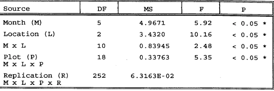
(57) 34. Source. DF I. Month (M). 5. 4.9671. 5.92. Location (L). 2. 3.4320. 10.16. M x L. 10. 0.83945. 2.48. Plot (P) MxLxP. 18. 0.33763. 5.35. 252. 6.3163E-02. Replication (R) MxLxPxR. MS < 0.05 * < 0.05 * < 0.05 * < 0.05 *. Table 4: Result of the ANOVA on the monthly 0.cf.venusta mean abundance during the period of April 1989 to September 1989, testing the Null Hypothesis : Ho, : There is no significant difference among Months Ho, : There is no significant difference among Locations Ho, : There is no interaction effect between Month and Location Ho4 : There is no significant difference between Plots Data were transformed to Log (x + 1) * : significant ..

(58) Figure 6 a, b, c: Monthly 0.cf.venusta mean abundance at location 1, 3, and 5..

(59) 35. 100 n -B. Location 1. n.I6. n -B. 80 n-B. n-16. 60. n-16. Pi. 40. n-15 a. n-16. n-B. 20 r.. n-. Number o findiv idu a ls per b lade. 0. a-16. Oct Nov Dec Jan Feb Mar Apr May Jun Jul Aug Sep I 1988 1989. 100. Location 3. 80. 60 n-16 n.6. n-16. 40 n 6. n.6. n-to. n.6. n-16. n-16. 20 n-B. n.16. Oct Nov Dec Jan Feb Mar Apr May Jun Jul Aug Sep 1988 I 1989 120. Location 5. 100 80 60. 40 n-8. II-6. n-6. 20 II. 0. n-B -6. n-16 n-11. nqo ..!.. Oct Nov Dec Jan Feb Mar Apr May Jun 1988 1989. Months of sampling n = number of blades observed 1= standard deviation -. n-16 n-16. n-ip. a-16. Jul Aug Sep.

(60) Figure 7 a, b, and c: Monthly 0.cf.venusta density at location 1, 3, and 5..

(61) 36. Number of in div idua ls Imm. 3.5 n.16 n. Location 1. n-16 2.5 n-16. n -6 1.5. n-8. n-8. n.t. n-6 n.•. 0.5. -0.5. n•I. Oct Nov Dec Jan Feb Mar Apr May Jun Jul I. 1988. Aug Sep. 1989. n-16 2.6 n-6. Location 3. 1.6 n-5. n-16 n. n-6. 0.5. n-a. nn-. -0.5. Oct Nov 1988. Dec. I. n-16 :11. n.16. Jan Peb mar Apr may Jun Jul Aug Sep 1989. 2.8. Location 5. 2 n-16. 1.6. n-16. n. 0.5. I.. r. Il. n-16 n-16. n-11. n-10. n'a. —. n-10. n. n. 0. Oct. •. Nov Dec Jan Feb Mar 1988. Apr May Jun 1969. Months of sampling n = number of blades observed I = Standard deviation. Jul Aug Sep.

(62) Figure 8 a, b, and c: Monthly mean area of seagrass blade at location 1, 3, and 5..

(63) 37. 100. 80. n-a. T. 00. n-8. a. n-lb n-le. Location 1. n.e. n-a. n-la 40. n-I6. n-a. . ... nvia -. 20. 0. Oct. Nov. Dec. Jan. Feb Mar. Apr. 1988. May Jun. Jul. Aug Sep. 1989. Area ofblades (mm ). 00. 80 nM. n.8. n-ie n-10. n-16. n-8. n-a. Location 3. PI. 00 n-B. 40. OP. Tr•Hs 4. n-le. I!. 20. 0. !el. Oct. Nov8 Dec Jan 19 8. Feb Mar Apr May Jun 1089. Jul. Aug Sep. 1 00. 80 n.8. n-8 60. Location 5. rtnal. n-8. n-B. n••16. n-8. a-tb. 40. -. rvna. n-14. n-16. .• PI. 20. 0. Oct Nov Deo Jan Peb Mar 1988 I. Apr May Jun 1989. Months of sampling. n = number of blades observed I = Standard deviation. Jul. Aug Sep.

(64) 38. November 1988, June and July 1989. The area of the individual seagrass blades was higher at location 1 (33.34 mm 2 ) compared with the blades at locations 2 and 3 where their average areas were 29.76 and 27.67 mm2 respectively (see figure 8a. b, c). Table 5 shows the correlation coefficient for the relationship between the average abundance of 0.cf.venusta and the average area of the seagrass blades. The correlation between these two variables are mostly significant (p<0.05). In March 1989, April 1989, May 1989 and August 1989, however, no significant correlation could be detected (p>0.05).. 3.4.3. Monthly temporal 0.cf.venusta abundance in relation to the temporal abundance of the blades.. Experiment 2 which was designed to recognise the relationship between the abundance of 0.cf.venusta and the abundance of the seagrass blades, revealed significant relationship between these two factors (p<0.05, see tables 6 and 7). The relationship could also be clearly observed in figures 9 and 10. The analysis of variance of the temporal abundance of seagrass blades is shown in table 8. The later table also suggests that the seagrass blades were significantly different between times or dates of sampling (p<0.05). There was, however, no significant.

(65) 39. difference detected between plots in terms of the abundance of the seagrass blades (p>0.05).. 3.5. Discussion. 0.cf.venusta lives on the blades of both seagrass Halophila ovalis and Halodule uninervis. The statistical analysis, however, shows that 0.cf.venusta preferred to live on the blades of H.uninervis. Faber (1991) suspected the existence of substances that were exuded by the rhizomes of seagrass plants in explaining the foraminifera substrate preference in the Halophila meadows. He found that the epiphytic foraminifera Peneroplis planatus preferred to live on the horizontal rhizome and stems rather than the erect blades or sediments. This phenomenon was not investigated in this work, and it is not known if a particular seagrass species produces special substances to attract 0.cf.venusta. However, this study suggests. that the seagrass preference may be governed by the living nature and shape of blades of the two seagrass species..

(66) 40. Month of sampling October. r. 1988. 0.4580. November 1988. 0.5148. December 1988. 0.4520. January. 1989. 0.4731. February 1989. 0.3280. March. 1989. -0.0281 ns. April. 1989. -0.2225 ns. May. 1989. 0.0460 ns. June. 1989. 0.5592. July. 1989. 0.6529. August. 1989. September 1989. Table 5: Summary of the simple between the O.cf.venusta blades (n=48), testing Ho Ha. -0.2817 ns 0.5173. correlation coefficients abundance and the area of :p = 0 against :p 4 0. p = correlation coeficient in the population r = correlation coefficient in the sample r (0.05)2.46 = 0.285 ns= non significant.

(67) 41. Source Regression. DF. I. MS. 1. 9.4538E+05. Residual. 16. 3.1929E+05. Total. 17. F. 4.74. P. R2. <0.05* 0.2284. Table 6: Result of the ANOVA on regression between the number of 0.cf.venusta and the number of blades per 18 plots (1 plot = 78.53 cm2 ) during the period of October 1988 to March 1989, testing the Null hypothesis : Ho : there is no significant simple regression between the number of O.cf.venusta and the number of blades * : significant ..

(68) 42. Source Regression. I. DF 1. Residual. 34. Total. 35. MS. 3.4920. I. F 11.36**. P. R2. <0.01 0.2504. 3.0751E-01. Table 7: Result of the ANOVA on regression between the number of O.cf.venusta and the number of blades per 36 plots (1 plot = 78.53 cm 2 ) during the period of April to September 1989, testing the Null hypothesis Ho : there is no significant simple regression between the number of O.cf.venusta and the number of blades ** : highly significant ..

(69) 43. Source. DF. Month (M). 5. 410.51. 3.78. < 0.05 *. Plot (P). 1. 25.00. 0.23. > 0.05. M x P. 5. 174.60. 1.61. > 0.05. 24. 108.56. Replication (R) MxLxR. MS. F. P. Table 8: Result of the ANOVA on the monthly blades abundance during the period of April 1989 to September 1989, testing the Null Hypothesis : Ho,1 : There is no significant difference among Months Ho 2. :. Ho 3. :. There is no significant difference between Plots There is no interaction effect between Month and Plots. * : significant ..

(70) Figure 9: Number of 0.cf.venusta vs number of seagrass blades per plot in experiment 2 during October 1988 to March 1989.. Figure 10: Number of 0.cf.venusta vs number of seagrass blades per plot in experiment 2 during April 1989 to September 1989..

(71) Log ( N.O.V + 1). 44. 2.6. 2.6. Y = 2.62 +0.001 X 20. 40. 60. BO. 100. Log ( N.O.V + 1). Number of seagrass blades per plot. Number of seagrass blades per plot. N.O.V. = Number of a cf venusta. 120.

(72) 45. H.uninervis has relatively long, ligulate blades whereas H.ovalis has short rounded blades. The blades of. H.uninervis were also noted to be mostly in the erect position in the water column, whilst the blades of H.. ovalis tend to lie close to the sediment surface. In addition, it was also observed that most of the time. H.uninervis blades were found free from sediment particles, whilst the opposite condition occurred on the blades of H.ovalis. Clinging on the erect blade in the water column and free from sediment particles is possibly the ideal living condition for 0.cf.venusta. The abundance and density data, which were gathered for a one year period, during October 1988 to September 1989 suggest that 0.cf.venusta exhibited different periodicity in different locations. Thus, the abundance of 0.cf.venusta was seemingly not solely ruled by time, but also by a space factor. The space factor could be on a big scale, such as the location of sampling, or on a small scale, such as seagrass blades. The results from the close observation of three locations (1, 3 and 5) highlighted the importance of space on the bigger scale (macrospace) in regulating the. 0.cf.venusta population. Location 1, in which the average area of seagrass blades was relatively higher, exhibited greater abundance and density of 0.cf.venusta compared with the other two locations. In addition, the significant relationship between the number of. 0.cf.venusta and the area of seagrass blades) and also.

(73) 46. the results from experiment 2, that emphasized the the relationship between the number of blades and the number of O.cf.venusta) indicates, even more, the importance of microspace (the blades) in governing the epiphytic foraminiferal population. Severin (1983 and 1987) reported that, in Papua New Guinea, there was no correlation between seagrass area and Marginopora vertebralis density. The present study, therefore highlights that there are specific behavioural differences between two tropical epiphytic foraminiferal species in terms of their relationship with the seagrass as their substratum. During the course of investigation, it was noted that during the low tides, location 1 was always inundated longer compared with the other two locations. In addition, the seagrasses in location 1 appeared to remain covered by seawater during the low tide, whilst location 3 and 5 were exposed. It was also noticed that the seagrasses in location 1 were more dense compared with locations 3 and 5. Thus, it is reasonable to assume that the local conditions of depth, the density, and area of seagrass blades, singlely or together, play an important role in regulating the 0.cf.venusta population. There are at least three strong possibilities which must be taken into account in explaining the patchyness of the spatial distribution of 0.cf.venusta and their temporal fluctuations. These possibilities are : 1) the.

(74) 47. effect of the environmental factors ( e.g. waves and currents ) in detaching the foraminifera from the seagrass blades, 2) the migration of foraminifera between blades and 3) the natural development and reproduction of the epiphytic foraminiferal population. The effect of waves and currents can be inferred from the data gathered during the tropical cyclone season ( February 1989 to April 1989 ). The population of foraminifera decreased dramatically, especially in April 1989, when specimens were collected just one day after the tropical cyclone Aivu passed close to the study site. The possibility of foraminiferal migration is investigated in Chapter V section 3, and the reproduction and population development is discussed in chapter V section 1..

(75) 48. Chapter IV. Morphology of Osangularia cf.venusta :its abnormality and uses in the temporal study. 4.1. General morphology of 0.cf.venusta.. 4.1.1. Introduction. Foraminiferal classification, according to Loeblich and Tappan (1964, 1988) is based mainly on the characteristics of the test . These characteristics include chamber form, chamber arrangement, ornamentation, apertural structure, chamber wall composition, crystal form, lamellar character, perforation , canal system and internal modifications such as endoskeletal pillars and toothplates. There are many variations of foraminiferal chamber form such as globular, ovate, pyriform, tubular, cyclical, hemispherical, radial, elongate, angular, tubuluspinate and fistulose. The arrangement of the chambers may be rectilinear, arcuate, zigzag, planispiral, peneropline, trochospiral, piano-convex, streptospiral, milioline, uniserial, biserial, triserial and quadriserial ( Loeblich and Tappan, 1964 ). Brasier (1980) and Haynes (1981) mentioned that in some cases.

(76) 49. one species of foraminifera can have more than one chamber arrangement , for instance planispiral in the early juvenile chambers and biserial in the later chambers, as is found in Spiroplectamina. In Eagerella, the juvenile has trochospiral chambers and the adult has a triserial chamber arrangement. The test of foraminifera may develop some variations of external surface ornamentation such as spines, keels, rugae, striae, costae, granules or reticulate and pustules ( Brasier, 1980). Other ornamentation described as punctate, limbate sutures, ribbed , fissures and pitted can also be found in foraminiferal tests (Loeblich and Tappan, 1964). Foraminifera have two main openings on their tests. The main aperture and the supplementary aperture, or its modification such as canal opening and pores. The aperture is highly variable but often species specific ( Loeblich and Tappan, 1964). Some additional modification such as lip, tooth, plates, rims, tegilla, bullae , phialine, umbilical teeth and umbilical bos may also be found ( Loeblich and Tappan, 1964; Boltovskoy and Wright, 1976; Brasier, 1980 ). Boltovskoy and Wright (1976) stated that the chamber wall may be constructed in 4 ways: 1) chitinious, 2) agglutinated, 3) calcareous and 4) silicious. The calcareous foraminifera have six wall structures : 1) microgranular walls, 2) procellaneous walls, 3) radial hyaline walls, 4) finely granular.

(77) 50. hyaline walls, 5) monocrystalline walls and 6) spicular walls. The finely granular hyaline walls have a lamellar structure when a thin section of the test is studied with light or electron microscope. These lamellar structures are monolamellar, rotaliid, bilamellar, and multilamellar ( Loeblich and Tappan, 1964; Boltovskoy and Wright, 1976 and Haynes, 1981). The "rotaliid" wall is unique because when new chambers form, a layer of the ultimate chamber also covers the apertural face of the penultimate chamber and forms a septal flap . This structure is slightly different to the bilamellar chamber structure in which the apertural face of the penultimate chambers is not covered by the new layer of shell material of the ultimate chamber ( Loeblich and Tappan, 1964; Boltovskoy and Wright, 1976; Brasier, 1980; Haynes, 1981). Haynes (1981) stated that the inner layer of the ultimate chamber in the "rotaliid" wall structure can modify the intercameral foramen and create a toothplate in the penultimate chamber. In asterigerinids, Hansen and Reiss (1972) found that the toothplate was formed by a doubled inner lining of the chamber wall. This toothplate separated the chamber lumen from the stellarchamberlet. Hottinger et.al (1991), however, emphasized that there is no association between toothplate and stellar-chamberlet, instead, they introduced the term umbilical plate for a structure that separates the chamber lumen from the foliar or stellar-chamberlet..

(78) 51 They also highlighted that the toothplate always protrudes distally and adaxially with a free edge through the main aperture. Billman, Hottinger and Osterle (1980) in their work on rotaliid foraminifera emphasized other internal chamber structures such as the foraminal plate and umbilical cover plate. They defined the foraminal plate as an inward oblique extension of chamber wall, running through the intercameral foramen and thus forming the umbilical cover plate. Hottinger et.al. (1991) separated the umbilical plate and cover plate from the umbilical cover plate, defined by Billman et.a1.(1980). According to Hottinger et.al. (1991) the umbilical plate is only found in the ultimate chambers because it extends from the distal to proximal chamber wall and is attached to the intercameral foramen and to the main aperture without protruding into it. A cover plate is never found in the ultimate chamber. It completely separates the main chamber lumen from the foliar chamberlet and no perforations exist in this plate. The perforations or pores in the chamber walls have been noted for a long time in the calcareous foraminifera. Based on the diameter of the pores, Boltovskoy and Wright (1976) stated that, there are at least two groups of calcareous foraminifera. The first group are Nodosariidae, Buliminidae, Polymorphinidae, and Heterohelicidae that have pores with diameter ranges from 1-6 A. The second group are Rotaliidae,.

(79) 52. Acervulinidae, and Nonoionidae with pores ranging from 6-15 A. Haynes (1981) stated that externally the pores could have an oval, round or slit-like shape. He also mentioned that the internal openings of pores in the chamber lumen are usualy larger in diameter than the external openings. The real function of the pores, according Boltovskoy and Wright (1976) still needs to be clarified. Berthold (1976, in Haynes, 1981) and Boltovskoy and Wright (1976), however, stated that some functions of the pores were to allow : a) the process of osmoregulation, b) gas exchange, c) excretion of dissolved organic substances, d) gamete release and d) especially in planktonic foraminifera, to increase buoyancy. The present study attempts to describe the general morphology including both the external and internal appearence of the calcareous foraminifera. Osangularia.cf .venusta (Brady). This description is very important as it ensures that the biology of only one species is described and the correct taxonomic position of 0.cf.venusta is determined.. 4.1.2. Material and methods. Live specimens were used for observing the morphology of the forams. To do this, live specimens of.

(80) 53. the seagrass Halodule uninervis, upon which the foraminifera is epiphytic, were collected from Shelly Bay. The blades were immersed in filtered seawater and the live forams photographed. The morphology of 0.cf.venusta was also studied by using dry specimens immersed in aniseed oil. Pictures were taken by using a camera connected to a light microscope, using both transmitted and reflected light. Detailed observations of the external and internal features of O.cf.venusta test were carried out by means of scanning electron microscopy (Phillips XL 20) in the SEM unit, James Cook University.. 4.1.3. Results. 4.1.3.1. Megalospheric and microspheric morphology. 0.cf.venusta has a low trochospiral chamber. arrangement with no carina or keel, and may be coiled either sinistrally or dextrally. All chambers are visible from the dorsal side, whilst only the chambers from the last whorl are visible from the ventral side. The megalospheric and microspheric specimens were differentiated by measuring the diameter of the first chamber (proloculus). The proloculus diameter of the megalospheric specimens ranged from 40 to 80 A, whereas the diameter of the proloculus of the microspheric forms ranged from 5 to 10 A. The microspheric forms have more.

No results found