Managing the effect of infiltration variability on the performance of surface irrigation

(1)

U

NIVERSITY OF

S

OUTHERN

Q

UEENSLAND

Faculty of Engineering and Surveying

Managing the Effect of Infiltration

Variability on the Performance of Surface

Irrigation

A dissertation submitted by

Malcolm Horace Gillies

For the Award of

Doctor of Philosophy

(2)

ii

ABSTRACT

Infiltration variability is a major issue during the design phase and management for all

types of irrigation systems. Infiltration is of particular significance for furrow

irrigation and other forms of surface irrigation as the soil intake rate at any given

position not only determines the depth applied but also governs the distribution of

water to other locations in the field. Despite this, existing measurement and evaluation

procedures generally assume homogeneous soil infiltration rates across the field to

simplify data collection and computational requirements. This study was conducted to

(a) determine whether spatial and temporal variations in soil infiltration characteristics

have a significant impact on the performance of surface irrigation and (b) identify

more appropriate management strategies that account for this variability and

substantially improve irrigation performance.

The soil infiltration rate is typically expressed as an empirical function of opportunity

time. The infiltration function parameters cannot be directly measured but are

commonly estimated from field hydraulic measurements using an appropriate

simulation model. The volume balance model as used in the inverse solution for

infiltration (e.g. Two Point Method) was modified to enable runoff data collected

during the inflow period to be used in the estimation of the infiltration parameters.

The resulting model, IPARM also accommodates the full (variable) inflow

hydrograph rather than relying on a constant inflow assumption. Inclusion of runoff

data in the inverse solution improved the accuracy of the infiltration curve during the

runoff phase and hence offered the greatest benefit where the irrigation time exceeded

the completion of advance. Analysis of field data collected from multiple furrows at a

single site indicated that accounting for the variable inflow in IPARM both reduced

the variability (e.g. reduction in the coefficient of variance (CV) of cumulative

infiltrated depths of 18.6% and 11.5% at opportunity times of 100 and 500 minutes,

respectively) and standardised the shape of the estimated infiltration curves. Hence, a

significant proportion of the apparent variability in soil infiltration rates was shown to

be a consequence of the constant inflow assumption. Sensitivity analysis indicated

that IPARM is highly sensitive to the runoff measurements but is not influenced by

(3)

iii

estimated infiltration parameters using the full hydrodynamic model SIRMOD

showed that the inclusion of runoff data in the inverse procedure did not compromise

the ability to predict the measured advance trajectory but significantly improved the

fit to the measured runoff volumes (average decrease in absolute error of simulated

runoff volumes of 84%). Whereas the use of runoff data enabled SIRMOD to estimate

runoff volumes, accounting for variable inflow improved the fit of the predicted

runoff rates to the shape of the measured outflow hydrograph.

Field data collected from several sites across the Darling Downs, Queensland has

shown that the infiltration rates vary significantly (e.g. by up to 65% at 500 minutes),

both spatially between furrows and temporally over the season. For the sites studied,

the spatial variance in infiltration was surpassed by the seasonal variance (e.g. average

CV of infiltration of 33.1% compared to 12.5%) but no consistent trends were

identified. It was found that the lognormal distribution provided the best fit for the

variance in the infiltration curves which was in turn strongly related to the statistical

distribution of the infiltration term of the volume balance. From this research, a

procedure was developed to predict the infiltration parameters using a single advance

point and any number of “known” infiltration curves from the same field.

The IrriProb model was developed to extend the process of simulation from a single

furrow scale to the whole field scale. IrriProb performs the full hydrodynamic

simulation for multiple independent furrows which are combined to form a spatial

representation of the water application. Each furrow can have a unique infiltration

rate, inflow rate (Q), time to cut off (TCO) and soil moisture deficit. Validation of

IrriProb using multiple sets of field data demonstrated that the single furrow

simulations failed to predict the true whole field irrigation performance (e.g. furrow

distribution uniformity (DU) between 72.2% and 86.2% compared to the whole field

DU of 64.8%).

An optimisation routine was developed within IrriProb to maximise irrigation

performance through identification of optimal values of Q and TCO. The optimisation

(4)

iv

performance criteria. The user selects the appropriate performance terms and the

optimal management is determined through a graphical overlay of the complying

ranges of Q and TCO. Hence, the objective function of IrriProb retains the importance

of each individual performance term, an advantage over those based on numerical

combinations of weighted terms. Simulation of the whole field application under

practical ranges of Q and TCO demonstrated the complex interactions between the

performance indices (e.g. the trade off between requirement efficiency (RE) and

application efficiency (AE)). In cases of low infiltration variability it was possible to

optimise the whole field performance using a single value of Q and TCO. However,

under increased infiltration variability it was more appropriate to manage the field

using two or more different management strategies. Irrigation optimisation based on

measurements from a single furrow or the average infiltration curve, cannot identify

the optimal combination of Q and TCO for the whole field. Simulation of field

management based on the optimisation strategy obtained from single furrow

measurements results in lower whole field performance than estimated from

simulation of the single furrow data (e.g. field RE, AE and distribution uniformity of

the root zone up to 26%, 18% and 66% lower than predicted). Field trials were used to

demonstrate the ability to estimate whole field infiltration variability, evaluate whole

field irrigation performance and optimise whole field irrigation management while

(5)

v

CERTIFICATION OF DISSERTATION

I certify that the ideas, designs, experimental work, software code, results, analyses

and conclusions presented in this dissertation are entirely my own effort, except

where otherwise indicated and acknowledged.

I further certify that the work is original and has not been previously submitted for

assessment in any other course or institution, except where specifically stated.

____________________________ ___________

Malcolm Horace Gillies, Candidate

Date

Endorsement:

____________________________ ___________

Prof. Rod Smith, Principal supervisor

Date

____________________________ ___________

(6)

vi

ACKNOWLEDGEMENTS

The completion of this research is a testimonial to the assistance I have received from

a great many people. I would like to take the time here to express my gratitude to

some of those who have helped and inspired me during the past three and a half years.

I would like to express my thanks to my supervisors Prof. Rod Smith and Prof. Steven

Raine for their guidance during the last few years. I sincerely thank them for their

enthusiasm, technical assistance and patience during my PhD studies. Finally I would

like to thank Steve and Rod for the proof reading of this dissertation, I know that my

English expression can be a little crude at the best of times.

To the staff at the NCEA for their support during my research and help in the

collection of irrigation data. In particular to Dr J. McHugh and Dr J. Eberhard for

assistance in collection of data for the Lagoona field trial. I would also like to thank

John Hornbuckle (CSIRO) for use of his field data. A major part of this research

would have not been possible without the simulation model and guidance provided by

David McClymont.

I acknowledge the scholarship funding provided by the University of Southern

Queensland and the Australian Federal Government. Also to the CRC for Irrigation

Futures for providing additional funding for operational costs. I am grateful to the

members of the CRC IF for their support and constructive criticism during my study.

To my brother and sisters and especially Mum and Dad who have encouraged me

throughout my life. I am forever indebted to you for all your support and inspiration

that has led me to this point.

Finally, to my wife Dennielle, words cannot express the appreciation I have for your

love and understanding over the past few years. To you Dennielle, I dedicate this

(7)

vii

LIST OF PUBLICATIONS FROM THIS

RESEARCH

Gillies, M.H. and Smith, R.J. (2005), Infiltration parameters from surface irrigation

advance and run-off data,

Irrigation Science

, Vol. 24, No.1, pp 25-35.

Gillies, M.H. and Smith, R.J. and Raine, S.R. (2006) Is it possible to extract

infiltration rates for variable inflow furrow irrigation? National Conference, Irrigation

Association of Australia. 9-11 May, Brisbane. pp 63-64.

Gillies, M.H. and Smith, R.J. and Raine, S.R. (2007), Accounting for temporal inflow

variation in the inverse solution for infiltration in surface irrigation,

Irrigation

(8)

Table of Contents

viii

TABLE OF CONTENTS

ABSTRACT ...II

CERTIFICATION OF DISSERTATION ... V

ACKNOWLEDGEMENTS ...VI

LIST OF PUBLICATIONS FROM THIS RESEARCH... VII

[image:8.595.112.526.427.730.2]

TABLE OF CONTENTS ... VIII

TABLE OF FIGURES... XV

LIST OF TABLES ...XIX

LIST OF ABBREVIATIONS ... XXII

LIST OF SYMBOLS ...XXIII

CHAPTER 1 INTRODUCTION ... 1

1.1 BACKGROUND... 1

1.1.1 Irrigation... 1

1.1.2 Irrigation Performance... 2

1.1.3 Surface Irrigation... 3

1.1.4 Irrigation in Australia ... 6

1.1.5 The Surface Irrigation Debate ... 8

1.1.6 The Issue of Infiltration Variability ... 10

1.2 HYPOTHESIS... 11

1.3 OBJECTIVES... 11

1.4 STRUCTURE OF THIS DISSERTATION... 11

CHAPTER 2 REVIEW OF INFILTRATION AND INFILTRATION VARIABILITY ... 13

2.1 INTRODUCTION... 13

2.2 INFILTRATION... 13

2.2.1 Infiltration Equations... 14

2.3 FACTORS INFLUENCING INFILTRATION... 18

2.3.1 Soil Texture ... 19

2.3.2 Soil Erosion ... 21

2.3.3 Soil Structure and Compaction... 22

2.3.4 Soil Moisture Content and Cracking ... 25

(9)

CHAPTER 3 HYDRAULIC SIMULATION OF FURROW IRRIGATION... 69

3.1 PURPOSE OF THE SIMULATION MODEL... 69

3.1.1 Identification of Field Characteristics ... 69

3.1.2 Evaluation of the Current Irrigation Performance ... 69

3.1.3 Optimisation of Field Design and Management ... 70

3.2 HYDRAULIC MODEL THEORY... 70

3.2.1 Full Hydrodynamic Model ... 72

(10)

CHAPTER 4 DEVELOPMENT OF IPARM ... 90

4.1 INTRODUCTION... 90

4.2 VOLUME BALANCE MODEL FOR INVERSE SOLUTION OF INFILTRATION... 91

4.2.2 Advance Phase ... 91

4.2.3 Runoff Phase ... 97

4.2.4 Variable Inflow... 99

4.3 IPARMMODEL DEVELOPMENT... 101

4.3.1 Advance Phase ... 101

4.3.2 Runoff Phase ... 103

4.3.3 Depletion and Recession Phases... 105

4.3.4 Variable Inflow... 107

4.3.5 Objective function ... 111

4.3.6 Solution Scheme... 112

4.3.7 The IPARM Computer Software ... 115

4.4 EVALUATION OF IPARM ... 117

4.4.1 Input Data ... 117

4.4.2 Estimation of Infiltration Parameters... 121

4.4.3 Validation of the Surface Storage Smoothing Approach... 127

(11)

CHAPTER 5 FIELD VARIABILITY OF INFILTRATION... 150

5.1 INTRODUCTION... 150

5.2 PREVIOUS ATTEMPTS TO ASSESS INFILTRATION VARIABILITY... 151

5.3 DESCRIBING INFILTRATION VARIABILITY WITH STATISTICAL TECHNIQUES... 152

5.3.1 Review of Statistical Distribution Models... 152

5.3.2 Sampling Distribution, a Tool to Determine Required Number of Measurements ... 156

5.4 MULTIPLE FURROW FIELD DATA... 157

5.4.1 Collection of Field Data using Irrimate™ Equipment... 157

5.4.2 Downs... 159

5.4.3 Chisholm ... 160

5.4.4 Turner ... 160

5.4.5 Additional Field Data for Seasonal Trends... 161

5.4.6 Estimating Surface Storage using Manning’s n... 161

5.5 ESTIMATION OF THE INFILTRATION CURVES... 162

5.5.1 Downs... 162

5.5.2 Chisholm ... 163

5.5.3 Turner ... 164

5.6 VARIABILITY OF INFILTRATION... 166

5.6.1 Variability between Infiltration Curves ... 166

5.6.2 Seasonal (Between Irrigation Events) Infiltration Variability ... 167

5.6.3 Significance of Temporal and Spatial Variability ... 170

5.6.4 Seasonal Compared to Spatial Variability ... 171

5.7 MINIMUM NUMBER OF INFILTRATION CURVES REQUIRED TO ESTIMATE WHOLE FIELD VARIABILITY... 173

(12)

CHAPTER 6 WHOLE FIELD SIMULATION MODEL ... 202

6.1 INTRODUCTION... 202

6.2 COMPONENTS OF THE SIMULATION MODEL... 203

6.2.1 Introduction to IrriProb... 203

6.2.2 FIDO Simulation Engine ... 204

6.2.3 Calculation of Performance Parameters ... 206

6.2.4 Calculation and Visualisation of the Whole Field Performance... 210

6.3 SURFACE IRRIGATION OPTIMISATION FRAMEWORK... 212

6.3.1 Development of the Optimisation Tool ... 212

6.3.2 Validation of the IrriProb Simulation Model... 215

6.4 SIMPLE FURROW AVERAGES CANNOT REPRESENT THE FIELD PERFORMANCE... 216

6.5 IRRIGATION PERFORMANCE IN HETEROGENEOUS CONDITIONS UNDER MEASURED FIELD MANAGEMENT... 218

6.6 CONCLUSION... 220

CHAPTER 7 OPTIMISING IRRIGATION PERFORMANCE CONSIDERING INFILTRATION VARIABILITY... 222

7.1 INTRODUCTION... 222

7.2 THE FURROW IRRIGATION OPTIMISATION PROCESS... 223

7.2.1 Factors to Consider in Addition to the Standard Performance Terms ... 223

7.2.2 Existing Techniques to Optimise Irrigation Management ... 225

7.2.3 Optimising Irrigation Performance at the Field Scale ... 226

7.3 THE OPTIMISATION OBJECTIVE FUNCTION... 227

7.3.1 Arithmetic Objective Function ... 227

7.3.2 Boolean Objective Function ... 229

7.3.3 Optimisation Methodology... 230

(13)

CHAPTER 8 PRACTICAL DEMONSTRATION: THE LAGOONA FIELD TRIAL . ... 259

8.1 INTRODUCTION... 259

8.2 FIELD DATA... 259

8.3 CALIBRATION OF THE INFILTRATION CURVE... 262

8.3.1 Estimation of Infiltration Curves using IPARM... 262

8.3.2 Minimum Distance for Field Measurement... 263

8.3.3 Predicting Infiltration Parameters using the Final Advance Time... 265

8.4 OPTIMISING PERFORMANCE... 266

8.4.1 Current Performance ... 266

8.4.2 Optimising the Time to Cut-off ... 268

8.4.3 Optimising Inflow ... 269

8.5 SENSITIVITY OF OPTIMISATION PROCESS TO UNCERTAINTIES IN FIELD MEASUREMENTS.... 270

CHAPTER 9 CONCLUSIONS AND RECOMMENDATIONS... 272

9.1 CONCLUSIONS FROM THIS RESEARCH... 272

9.1.1 Estimation of Infiltration Parameters from Field Measurements... 272

9.1.2 Statistical Nature of Infiltration Variability... 274

9.1.3 Whole Field Simulation and Optimisation Model ... 275

9.2 KEY RESEARCH OUTCOMES... 278

9.3 RECOMMENDATIONS FOR FURTHER RESEARCH... 278

9.3.1 Inverse Techniques to Estimate Infiltration... 279

(14)

APPENDIX E RESULTS FROM SAMPLE SIZE ANALYSIS ... 346

APPENDIX F RESULTS FROM INFILTRATION PREDICTION... 349

APPENDIX G VALIDATION OF THE FIDO SIMULATION ENGINE USED BY IRRIPROB ... 352

APPENDIX H IRRIPROB: IRRIGATION PERFORMANCE UNDER MEASURED CONDITIONS... 358

(15)

Table of Figures

xv

TABLE OF FIGURES

Figure 1-1 Large scale level basin irrigation of rice/wheat field in Griffith region, southern

NSW ...5

Figure 1-2 Furrow irrigation of cotton near Moree, northern NSW showing siphon application ...5

Figure 2-1 Cross section view of the (a) single ring and (b) double ring infiltrometer (Reynolds et al. 2002) ...36

Figure 2-2 Sample inflow hydrographs for alternative inflow regimes ...58

Figure 3-1 Control volume for Saint-Venant equations...71

Figure 3-2 Screenshot of SIRMOD III: simulation of the Kooba field with variable inflow (infiltration estimated using advance and runoff with variable inflow) ...86

Figure 4-1 Volume balance model during the advance phase ...91

Figure 4-2 Explanation of the Surface Storage Smoothing calculation ...110

Figure 4-3 Screen shot of main user interface for IPARM version 1.1.2...116

Figure 4-4 Screen shot of main user interface for IPARM version 2 ...116

Figure 4-5 Measured inflow hydrographs for IPARM validation...119

Figure 4-6 Calibrated infiltration curves for IPARM validation...124

Figure 4-7 Cumulative infiltrated volumes comparing infiltration from the volume balance (actual/measured) with predicted infiltration from parameters estimated from the advance and storage phases ...126

Figure 4-8 Comparing infiltration curves estimated using the variable inflow hydrograph between original surface storage and surface storage smoothing (SSS) technique ...128

Figure 4-9 Comparing the surface storage smoothing (SSS) calculation with the standard variable and constant inflow approach (Merungle Hill data) ...129

Figure 4-10 Measured and SIRMOD simulated advance (Benson data) ...131

Figure 4-11 Measured and SIRMOD simulated advance (Printz data) ...131

Figure 4-12 Measured and predicted runoff hydrographs using different infiltration parameters ...134

Figure 4-13 Effect of infiltration parameter estimation on the predicted water depth profile (Merungle Hill data)...137

Figure 4-14 Measured inflow hydrographs for Kooba site ...138

Figure 4-15 Infiltration curves for the Kooba site estimated using advance data with constant inflow ...139

(16)

[image:16.595.107.527.36.756.2]

Table of Figures

xvi

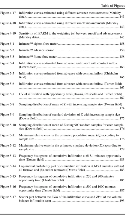
Figure 4-17 Infiltration curves estimated using different advance measurements (Merkley

data)...143

Figure 4-18 Infiltration curves estimated using different runoff measurements (Merkley data)...143

Figure 4-19 Sensitivity of IPARM to the weighting (w) between runoff and advance errors (Merkley data) ...145

Figure 5-1 Irrimate™ siphon flow meter ...158

Figure 5-2 Irrimate™ advance sensor...158

Figure 5-3 Irrimate™ flume flow meter ...158

Figure 5-4 Infiltration curves estimated from advance and runoff with constant inflow (Downs field)...163

Figure 5-5 Infiltration curves estimated from advance with constant inflow (Chisholm field) ...165

Figure 5-6 Infiltration curves estimated from advance with constant inflow (Turner field) ...165

Figure 5-7 CV of infiltration with opportunity time (Downs, Chisholm and Turner fields) ...167

Figure 5-8 Sampling distribution of mean of Z with increasing sample size (Downs field) ...174

Figure 5-9 Sampling distribution of standard deviation of Z with increasing sample size (Downs field)...175

Figure 5-10 Sampling distribution of mean of Z using 900 random samples for each sample size (Downs field) ...176

Figure 5-11 Maximum relative error in the estimated population mean (Eµ) according to sample size ...178

Figure 5-12 Maximum relative error in the estimated standard deviation (Eσ) according to sample size ...179

Figure 5-13 Frequency histograms of cumulative infiltration at 615.1 minutes opportunity time (Downs field) ...183

Figure 5-14 Log-normal probability plot of cumulative infiltration at 615.1 minutes with (a) all furrows and (b) outlier removed (Downs field) ...183

Figure 5-15 Frequency histograms of cumulative infiltration at 230 and 800 minutes opportunity time (Chisholm field)...185

Figure 5-16 Frequency histograms of cumulative infiltration at 500 and 1000 minutes opportunity time (Turner field) ...187

(17)

[image:17.595.106.526.47.770.2]

Table of Figures

xvii

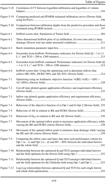
Figure 5-18 Correlation of CV between logarithm infiltration and logarithm of volume balance...194

Figure 5-19 Comparing predicted and IPARM estimated infiltration curves (Downs field, using Irr1Fur1) ...196

Figure 5-20 Comparison between infiltration depths from the predictive procedure and those estimated using IPARM (actual) ...197

Figure 6-1 IrriProb screen shot: Simulation of Turner field ...204

Figure 6-2 Three dimensional IrriProb plots of (a) infiltration, (b) root zone and (c) deep drainage (Downs trial site under measured conditions) ...211

Figure 6-3 Batch simulation parameter input box...212

Figure 6-4 Screenshot from IrriProb: Performance indicators for Downs field (Q = 1 to 11 L s-1 and TCO = 200 to 1200 minutes)...213

Figure 6-5 Screenshot from IrriProb continued: Performance indicators for Downs field (Q = 1 to 11 L s-1 and TCO = 200 to 1200 minutes) ...214

Figure 6-6 IrriProb screen shot: Using the optimising tool to determine inflows that achieve RE>90%, DURZ>90% and AE>65% (Downs field)...214

Figure 7-1 Optimising using an Arithmetic objective function: ¼(RE) ¼AE) + ¼DU + ¼(1-DD%) (Downs field)...228

Figure 7-2 Cut-off time plotted against application efficiency and requirement efficiency (Downs field)...232

Figure 7-3 Inflow rate plotted against application efficiency and requirement efficiency (Downs field)...233

Figure 7-4 Behaviour of the objective function of a) Opt 1 and b) Opt 2 (Downs field) .235

Figure 7-5 Behaviour of AE in relation to RE and DURZ (Downs field) ...236

Figure 7-6 Behaviour of DDD in relation to RE and AE (Downs field)...236

Figure 7-7 Movement of the optimal inflow point to maximise application efficiency while varying the RE and DURZ criteria (Downs field)...238

Figure 7-8 Movement of the optimal inflow point to minimise deep drainage while varying the RE and AE criteria (Downs field) ...239

Figure 7-9 Comparing the inflow rates and times that meet each performance criteria for Opt 1 (a – c) and Opt 2 (c - d) and DU = 80% between the individual furrows and the whole field ...241

Figure 7-10 Relationship between the optimised Q and TCO amongst individual furrows and the field optimum for the Downs field using Opt 1...252

Figure 7-11 Relationship between the optimised Q and TCO amongst individual furrows and the field optimum for the Chisholm field using Opt 1 and Opt 2 ...253

(18)

Table of Figures

xviii

Figure 8-1 Advance meter at 0 m (head-ditch) in Lagoona trial...260

Figure 8-2 Lagoona field trial layout ...261

Figure 8-3 Time taken to reach final advance point (761 m) for the Lagoona field ...262

Figure 8-4 Infiltration curves for Lagoona estimated using IPARM ...263

Figure 8-5 Correlogram of final advance times (761 m) for Lagoona...264

Figure 8-6 Predicted infiltration curves for Lagoona...266

Figure E.1 Chisholm: Sampling distributions of the mean ...347

Figure E.2 Chisholm: Sampling distributions of the standard deviation...347

Figure E.3 Turner: Sampling distributions of the mean...348

Figure E.4 Turner: Sampling distributions of the standard deviation ...348

Figure G.1 Simulated advance trajectories (Downs, Irr2 Fur3) ...354

Figure G.2 Simulated runoff hydrographs (Downs, Irr2 Fur3) ...354

(19)

List of Tables

xix

[image:19.595.105.526.44.766.2]

LIST OF TABLES

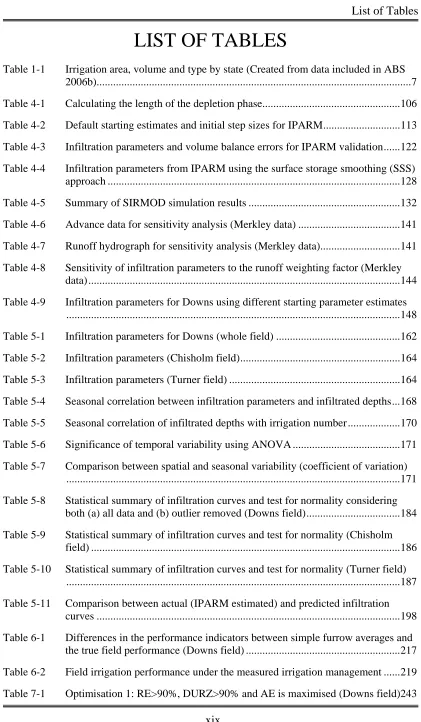
Table 1-1 Irrigation area, volume and type by state (Created from data included in ABS

2006b)...7

Table 4-1 Calculating the length of the depletion phase...106

Table 4-2 Default starting estimates and initial step sizes for IPARM...113

Table 4-3 Infiltration parameters and volume balance errors for IPARM validation...122

Table 4-4 Infiltration parameters from IPARM using the surface storage smoothing (SSS) approach ...128

Table 4-5 Summary of SIRMOD simulation results ...132

Table 4-6 Advance data for sensitivity analysis (Merkley data) ...141

Table 4-7 Runoff hydrograph for sensitivity analysis (Merkley data)...141

Table 4-8 Sensitivity of infiltration parameters to the runoff weighting factor (Merkley data)...144

Table 4-9 Infiltration parameters for Downs using different starting parameter estimates ...148

Table 5-1 Infiltration parameters for Downs (whole field) ...162

Table 5-2 Infiltration parameters (Chisholm field)...164

Table 5-3 Infiltration parameters (Turner field) ...164

Table 5-4 Seasonal correlation between infiltration parameters and infiltrated depths...168

Table 5-5 Seasonal correlation of infiltrated depths with irrigation number...170

Table 5-6 Significance of temporal variability using ANOVA ...171

Table 5-7 Comparison between spatial and seasonal variability (coefficient of variation) ...171

Table 5-8 Statistical summary of infiltration curves and test for normality considering both (a) all data and (b) outlier removed (Downs field)...184

Table 5-9 Statistical summary of infiltration curves and test for normality (Chisholm field) ...186

Table 5-10 Statistical summary of infiltration curves and test for normality (Turner field) ...187

Table 5-11 Comparison between actual (IPARM estimated) and predicted infiltration curves ...198

Table 6-1 Differences in the performance indicators between simple furrow averages and the true field performance (Downs field) ...217

Table 6-2 Field irrigation performance under the measured irrigation management ...219

(20)

List of Tables

[image:20.595.108.525.46.764.2]

xx

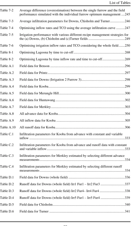
Table 7-2 Average difference (overestimation) between the single furrow and the field

performance simulated with the individual furrow optimum management ....245

Table 7-3 Average infiltration parameters for Downs, Chisholm and Turner...246

Table 7-4 Optimising inflow rates and TCO using the average infiltration curve ...247

Table 7-5 Irrigation performance with various different recipe management strategies for the (a) Downs, (b) Chisholm and (c)Turner fields ...249

Table 7-6 Optimising irrigation inflow rates and TCO considering the whole field ...250

Table 8-1 Optimising Lagoona by time to cut-off ...268

Table 8-2 Optimising Lagoona by time inflow rate and time to cut-off...269

Table A.1 Field data for Benson ...296

Table A.2 Field data for Printz...297

Table A.3 Field data for Downs (Irrigation 2 Furrow 3)...298

Table A.4 Field data for Kooba...299

Table A.5 Field data for Merungle Hill...300

Table A.6 Field data for Huntawang ...302

Table A.7 Field data for Merkley...303

Table A.8 All advance data for Kooba...304

Table A.9 All inflow data for Kooba ...305

Table A.10 All runoff data for Kooba...306

Table C.1 Infiltration parameters for Kooba from advance with constant and variable inflow ...333

Table C.2 Infiltration parameters for Kooba from advance and runoff data with constant and variable inflow...333

Table C.3 Infiltration parameters for Merkley estimated by selecting different advance measurements ...334

Table C.4 Infiltration parameters for Merkley estimated by selecting different runoff measurements ...334

Table D.1 Field data for Downs (whole field) ...336

Table D.2 Runoff data for Downs (whole field) Irr1 Fur1 – Irr2 Fur3 ...337

Table D.3 Runoff data for Downs (whole field) Irr2 Fur4– Irr4 Fur4 ...338

Table D.4 Runoff data for Downs (whole field) Irr5 Fur1 – Irr5 Fur4 ...339

Table D.5 Field data for Chisholm...340

(21)

List of Tables

[image:21.595.109.525.24.696.2]

xxi

Table D.7 Field data and infiltration parameters for Coulton A ...342

Table D.8 Field data and infiltration parameters for Coulton B...343

Table D.9 Field data for and infiltration parameters for Coulton C ...344

Table D.10 Field data and infiltration parameters for Turner Field 18 ...345

Table F.1 Estimated infiltration parameters for Downs ...350

Table F.2 Estimated infiltration parameters for Chisholm ...350

Table F.3 Estimated infiltration parameters for Turner...351

Table G.1 Comparison of SIRMOD and IrriProb Performance Terms...356

Table H.1 Downs: irrigation performance under measured conditions ...359

Table H.2 Chisholm: irrigation performance under measured conditions using a constant deficit equal to 0.06 m...359

Table H.3 Chisholm: irrigation performance under measured conditions using measured (variable) soil water deficits ...360

Table H.4 Turner: irrigation performance under measured conditions ...360

Table I.1 Downs Opt 2: RE>95%, AE>70% and DDD is minimised ...362

Table I.2 Chisholm Opt 1: RE>90%, DURZ>90% and AE is maximised ...363

Table I.3 Chisholm Opt 2: RE>95%, AE>60% and DDD is minimised ...363

Table I.4 Chisholm Opt 3: RE>95%, AE>60% and DDD is minimised with variable irrigation requirement...364

Table I.5 Turner Opt 1: RE>90%,DURZ>90% and AE is maximised...365

Table I.6 Turner Opt 2: RE>95%, AE>70% and DDD is minimised...366

Table I.7 Recipe field performance ...367

Table J.1 Advance data for Lagoona Trial...369

Table J.2 Runoff data for Lagoona Trial...370

Table J.3 Infiltration parameters for Lagoona from IPARM ...371

Table J.4 Infiltration parameters predicted using final advance point ...372

(22)

List of Abbreviations

xxii

LIST OF ABBREVIATIONS

ADU absolute distribution uniformity

AE application efficiency

AELQ application efficiency of the low quarter

AER application efficiency accounting for tail water recycling

AT average advance time (time of the final advance point for a set of furrows)

CV coefficient of variation

CU Christiansen's uniformity coefficient

DD deep drainage/deep percolation below the root zone DDD average depth of deep drainage

DU low quarter distribution uniformity DURZ distribution uniformity of the root zone EC electrical conductivity

EM electromagnetic survey ESP exchangeable sodium percentage

ETc crop evapo-transpiration calculated from the reference evaporation

FIDO Furrow Irrigation Design Optimiser Fur furrow

GPS global positioning system

IPARM infiltration parameters from advance and runoff model Irr irrigation

MIC model infiltration curve

NCEA National Centre for Engineering in Agriculture NSW New South Wales

Opt optimisation (objective function to optimise performance) PAM Polyacrylamide

PRD partial root-zone drying

Q inflow rate Qld Queensland

RE requirement efficiency

RMSE root mean square error SAR sodium adsorption ratio SCS US Soil Conservation Service SSE standard square error

SSS surface storage smoothing (technique to estimate the surface storage term)

(23)

List of Symbols

xxiii

LIST OF SYMBOLS

α significance level

β curvature constant for surface water storage

γ semivariance

ζ empirical exponent of Q for variation of infiltration with inflow

η dynamic viscosity (Pa s)

θ decrease in infiltration over time from Horton equation

λ ratio of current time to end of advance µ population mean

σ population standard deviation

σs sample standard deviation

σy surface storage coefficient for advance

phase

σys surface storage coefficient for storage

phase

σz1 subsurface storage coefficient of the

transient infiltration term

σz2 subsurface storage coefficient of the

steady infiltration term

τ infiltration opportunity time (min)

0

f

τ

time constant of the Branched Kostiakov equation

φ empirical parameter for variation of infiltration with wetted perimeter

χ2

chi squared statistic

ωCV coefficient to calculate CVInfiltration from

CVVB

ωZVal coefficient to calculate ZValInfiltration from

ZValVB

a empirical Kostiakov/Modified Kostiakov infiltration parameter

A cross-sectional area of flow (m2)

A0 upstream area of flow (m2)

ACF autocorrelation coefficient

AT average time value of the last measured advance point (min)

c coefficient of the power relationship of furrow width to depth

C crack infiltration term (m3 m-1)

CVInfiltration time averaged CV for the

logarithm of the Modified Kostiakov infiltration

CVVB CV for the logarithm of the infiltration

term of the volume balance

D volume of infiltration per unit area of soil (m)

LQ

D

average of D over the quarter of the field with the lowest infiltration (m)

LQ RZ

D

average of DRZ over the quarter of the

field with the lowest infiltration (m)

DDD volume of deep drainage per unit area of

soil (m)

Dmin minimum value of D across the field (m)

Dreq required volume of infiltration per unit

area or soil moisture deficit (m)

DRZ volume infiltrated and stored in the root

zone per unit area of soil (m)

E[] the expected value

ER efficiency of the tail-water recycling

system

f0 semi-empirical steady state infiltration

parameter of the Modified Kostiakov (m3 m-1 min-1)

F rapid surface storage term from the Horton equation

FS scaling factor of infiltration function for

the MIC approach

g acceleration due to gravity (9.81 m s-2)

G group iteration factor (default = 0.01)

h lag distance (between samples)

H pressure head (m)

I infiltration rate (m3 m-1 min-1)

ICF irrigation condition factor

(24)

List of Symbols

xxiv

Jatemp record of Ja for the last round of

individual parameter searches

JC equivalent to Ja butfor C JCtemp equivalent to Jatemp butfor JC

Jf0 equivalent to Ja butfor f0

Jf0temp equivalent to Jatemp but for Jf0

Jk equivalent to Ja butfor k

Jktemp equivalent to Jatemp butfor Jk

k empirical Kostiakov/Modified Kostiakov infiltration parameter (m3 m-1 min-a)

K hydraulic conductivity (m3 m-2 min-1)

Ks saturated hydraulic conductivity (m3 m-2

min-1)

Kwet hydraulic conductivity at field capacity

(m3 m-2 min-1)

L field length (m)

m exponent of the power relationship of furrow width to depth.

n Manning roughness coefficient

N number of data points

Na number of advance points

Nr number of runoff points

OBJ objective function for optimisation of irrigation management

p parameter of the power advance function

P wetted perimeter (m)

P0 upstream wetted perimeter (m)

qr steady runoff rate (m3 min-1)

Q discharge (m3 s-1)

Q0 inflow rate at upstream end of furrow

(m3 min-1)

Qr outflow discharge (m3 s-1)

Qx flow rate at point x in a furrow (m3 s-1)

r exponent of power advance function

R Pearson correlation coefficient

s distance measured from the upstream end of the field (m)

sZ2 variance of Z

S sorptivity as present in the Phillip equation

S0 field slope

Sf friction slope

t time (min or sec)

tStat t statistic from the t-distribution

tx time taken to reach point x (min)

tw time taken for a change in upstream area

to have effect over the wetted furrow length (min)

Tadvance length of the advance phase at the

current time (min)

Tdepletion length of the depletion phase (min)

v flow velocity (m s-1)

vx flow velocity at point x (m s-1)

Vf volume surface storage at end of storage

phase (m3)

VI volume of infiltration (m3)

VR volume of runoff (m3)

i R

V

measured runoff volume at data point, i

(m3)

VS volume of surface storage (m3)

Vw velocity of a wave or small disturbance

(m s-1)

VZx volume of infiltration at the time tx (m3)

VolDD volume of infiltration that drains below

the rootzone as deep percolation (m3)

VolInfiltration volume of infiltration (m3)

VolRZ volume of infiltration stored in the root

zone (m3)

Volreq volume of infiltration required to refill

the rootzone (m3)

VolRunoff volume of runoff (m3)

VolInflow volume of inflow (m3)

w weighting factor for advance and runoff errors in IPARM (%)

W top width of flow within the furrow (m)

WB bottom width of the furrow (m)

WM furrow width at half the total height (m)

Ws furrow spacing (m)

WT furrow width at the total height (m)

x advance distance (m)

xi measured advance distance at data point,

(25)

List of Symbols

xxv

xt predicted advance distance if the

advance continued beyond the end of the field (m)

X a continuous variable

Xi a continuous variable measured at point i

y depth of flow (m)

y0 upstream depth of flow (m)

YT total height of furrow (m)

y

centroid of the area of flow (m)

yw depth of the wetting front (m)

Z infiltrated depth per unit length of furrow (m3 m-1)

ZS scaled infiltration depth per unit length

of furrow (m3 m-1)

Zx infiltrated depth at distance x (m3 m-1)

ZVal standard normal variate

ZValInfiltration time averaged ZVal for the

logarithm of the Modified Kostiakov infiltration

ZValVB ZVal for the logarithm of the infiltration

Managing the effect of infiltration variability on the performance of surface irrigation

NIVERSITY OF

types of irrigation systems. Infiltration is of particular significance for furrow

simplify data collection and computational requirements. This study was conducted to

The soil infiltration rate is typically expressed as an empirical function of opportunity

during the inflow period to be used in the estimation of the infiltration parameters.

the completion of advance. Analysis of field data collected from multiple furrows at a

be a consequence of the constant inflow assumption. Sensitivity analysis indicated

the ability to predict the measured advance trajectory but significantly improved the

Field data collected from several sites across the Darling Downs, Queensland has

identified. It was found that the lognormal distribution provided the best fit for the

The IrriProb model was developed to extend the process of simulation from a single

IrriProb using multiple sets of field data demonstrated that the single furrow

performance criteria. The user selects the appropriate performance terms and the

practical ranges of Q and TCO demonstrated the complex interactions between the

using two or more different management strategies. Irrigation optimisation based on

simulation of the single furrow data (e.g. field RE, AE and distribution uniformity of

and conclusions presented in this dissertation are entirely my own effort, except

Endorsement:

I would like to express my thanks to my supervisors Prof. Rod Smith and Prof. Steven

To the staff at the NCEA for their support during my research and help in the

David McClymont.

To my brother and sisters and especially Mum and Dad who have encouraged me

LIST OF PUBLICATIONS FROM THIS

Association of Australia. 9-11 May, Brisbane. pp 63-64.

TABLE OF CONTENTS ... VIII

1.1 BACKGROUND... 1

CHAPTER 2 REVIEW OF INFILTRATION AND INFILTRATION VARIABILITY ... 13

2.1 INTRODUCTION... 13

Table of Contents

2.4 MEASURING SOIL INFILTRATION... 34

2.7 ESTIMATING INFILTRATION RATES WHILE ACCOUNTING FOR INFILTRATION VARIABILITY... 51

2.9 CONCLUSION... 67

CHAPTER 3 HYDRAULIC SIMULATION OF FURROW IRRIGATION... 69

3.1 PURPOSE OF THE SIMULATION MODEL... 69

Table of Contents

3.3 ESTIMATING INFILTRATION THROUGH INVERSE SIMULATION OF SURFACE IRRIGATION... 76

3.5.1 SIRMOD ... 86

CHAPTER 4 DEVELOPMENT OF IPARM ... 90

4.1 INTRODUCTION... 90

4.4 EVALUATION OF IPARM ... 117

Table of Contents

4.6 INFLOW AS A SOURCE OF VARIABILITY IN SPATIAL ESTIMATES OF INFILTRATION... 137

CHAPTER 5 FIELD VARIABILITY OF INFILTRATION... 150

5.1 INTRODUCTION... 150

5.5 ESTIMATION OF THE INFILTRATION CURVES... 162

Table of Contents

5.8 DESCRIBING INFILTRATION VARIABILITY USING STATISTICAL DISTRIBUTION FUNCTIONS.. 181

CHAPTER 6 WHOLE FIELD SIMULATION MODEL ... 202

6.1 INTRODUCTION... 202

6.4 SIMPLE FURROW AVERAGES CANNOT REPRESENT THE FIELD PERFORMANCE... 216

CHAPTER 7 OPTIMISING IRRIGATION PERFORMANCE CONSIDERING INFILTRATION VARIABILITY... 222

7.1 INTRODUCTION... 222

Table of Contents

7.5 CAN THE OPTIMAL FIELD MANAGEMENT BE IDENTIFIED FROM A SINGLE FURROW? ... 240

7.7 OPTIMISING IRRIGATION MANAGEMENT IN HETEROGENEOUS CONDITIONS USING THE WHOLE FIELD APPROACH... 250

CHAPTER 8 PRACTICAL DEMONSTRATION: THE LAGOONA FIELD TRIAL . ... 259

8.1 INTRODUCTION... 259

8.5 SENSITIVITY OF OPTIMISATION PROCESS TO UNCERTAINTIES IN FIELD MEASUREMENTS.... 270

CHAPTER 9 CONCLUSIONS AND RECOMMENDATIONS... 272

9.1 CONCLUSIONS FROM THIS RESEARCH... 272

Table of Contents

APPENDIX E RESULTS FROM SAMPLE SIZE ANALYSIS ... 346

Table of Figures

Table of Figures

Table of Figures

List of Tables

List of Tables

List of Tables

List of Abbreviations

List of Symbols

List of Symbols

List of Symbols