ISSN 1546-9239
© 2007 Science Publications
Corresponding Author: Barat GHOBADIAN, Tarbiat Modares University, Tehran, Iran, P.O.Box: 14115-111, Tel: +98-21-8011001, Fax: +98 -21-8006544
756
Combustion Analysis of a CI Engine Performance Using Waste Cooking Biodiesel Fuel
with an Artificial Neural Network Aid
Gholamhassan NAJAFI, Barat GHOBADIAN, Talal F YUSAF and Hadi RAHIMI Tarbiat Modares University, P. O. Box: 14115-111, Tehran- Iran
Abstract: A comprehensive combustion analysis has been conducted to evaluate the performance of a
commercial DI engine, water cooled two cylinders, in-line, naturally aspirated, RD270 Ruggerini diesel engine using waste vegetable cooking oil as an alternative fuel. In order to compare the brake power and the torques values of the engine, it has been tested under same operating conditions with diesel fuel and waste cooking biodiesel fuel blends. The results were found to be very comparable. The properties of biodiesel produced from waste vegetable oil was measured based on ASTM standards. The total sulfur content of the produced biodiesel fuel was 18 ppm which is 28 times lesser than the existing diesel fuel sulfur content used in the diesel vehicles operating in Tehran city (500 ppm). The maximum power and torque produced using diesel fuel was 18.2 kW and 64.2 Nm at 3200 and 2400 rpm respectively. By adding 20% of waste vegetable oil methyl ester, it was noticed that the maximum power and torque increased by 2.7 and 2.9% respectively, also the concentration of the CO and HC emissions have significantly decreased when biodiesel was used. An artificial neural network (ANN) was developed based on the collected data of this work. Multi layer perceptron network (MLP) was used for nonlinear mapping between the input and the output parameters. Different activation functions and several rules were used to assess the percentage error between the desired and the predicted values. The results showed that the training algorithm of Back Propagation was sufficient enough in predicting the engine torque, specific fuel consumption and exhaust gas components for different engine speeds and different fuel blends ratios. It was found that the R2 (R: the coefficient of determination) values are 0.99994, 1, 1 and 0.99998 for the engine torque, specific fuel consumption, CO and HC emissions, respectively.
Key words: Alternative fuel, Biodiesel-diesel blends, Artificial Neural Network
INTRODUCTION
One hundred years ago, Rudolf Diesel tested vegetable oil as fuel for his engine. In 1930s and 1940s vegetable oils were used as diesel fuels, but only in emergency situations[1, 2]. Alternative fuels for diesel engines are becoming increasingly important due to diminishing petroleum reserves and the environmental consequences of exhaust gases from petroleum fuelled engines[3, 4]. A number of studies have shown that triglycerides hold promise as alternative diesel engine fuels. So, many countries are interested in that. For example, evaluation of the production of biodiesel in Europe since 1992 shows an increasing trend [5]. Waste vegetable oil methyl ester is a biodiesel. Biodiesel is defined as the mono alkyl esters of long chain fatty acids derived from renewable lipid sources. Biodiesel,
character[4]. Lee and his colleagues recently reported that using B20 in diesel engine reduced SO2 emissions which were 19.7 ± 2.5% lower than No. 2 fuel, while NOx emissions were similar[4]. Dorad and his co-workers results showed that using biodiesel resulted in lower emissions of CO up to 58.9%, CO2 up to 86%, excepting a case which presented a 7.4% increase, NO up to 37.5%, and SO2 up to 57.7%, with increase in emission of NO2 up to 81%, excepting a case which presented a slight reduction[4]. Among the attractive features of biodiesel fuel are: (i) it is plant-, not petroleum-derived, and as such its combustion does not increase current net atmospheric levels of CO2 a “greenhouse” gas; (ii) it can be domestically produced, offering the possibility of reducing petroleum imports; (iii) it is biodegradable; and (iv) relative to conventional diesel fuel, its combustion products have reduced levels of particulates, carbon monoxide, and, under some conditions, nitrogen oxides. It is well established that biodiesel affords a substantial reduction in SOx emissions and considerable reductions in CO, hydrocarbons, soot, and particulate matter (PM). There is a slight increase in NOx emissions, which can be positively influenced by delaying the injection timing in engines [4, 10, 11]. From the available literature regarding the use of biofuel blends in IC engines, it is obvious that one has to overcome the obstacles encountered in actual operating conditions. Understanding and implementing these technical know how and reaching to the solid conclusions was the main objective of the present investigation, the results of which is depicted in the present paper. The actual engine performance is the core objective while using biofuel blends. Artificial neural networks (ANN) are used to solve a wide variety of problems in science and engineering, particularly for some areas where the conventional modeling methods fail. A well-trained ANN can be used as a predictive model for a specific application, which is a data-processing system inspired by biological neural system. The predictive ability of an ANN results from the training on experimental data and then validation by independent data. An ANN has the ability to re-learn to improve its performance if new data are available[12]. An ANN model can accommodate multiple input variables to predict multiple output variables. It differs from conventional modeling approaches in its ability to learn about the system that can be modeled without prior knowledge of the process relationships. The prediction by a well-trained ANN is normally much faster than the conventional simulation programs or mathematical models as no lengthy iterative calculations are needed to solve differential equations using numerical methods but the selection of an appropriate neural network topology is important in terms of model accuracy and model simplicity. In
addition, it is possible to add or remove input and output variables in the ANN if it is needed. The objective of this study was to develop a neural network model for predicting engine parameters like emission, fuel consumption and torque in relation to input variables such as engine speed and biofuel blends. This model is of a great importance due to its ability to predict engine performance under varying conditions.
MATERIALS AND METHODS
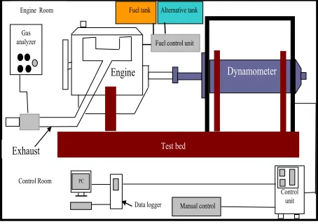
In the present investigation, biodiesel was produced from waste vegetable oil of MEGA Motors Co. restaurant. 1.8 gr KOH (as Alkali catalyst) and 33.5cc methanol (as an alcohol) was applied for 120 gr waste vegetable oil in this reaction. Biodiesel production reaction time was 1 hour with stirring and no heat. Up to one week time needs for separation and washing process. The Waste vegetable oil methyl ester was added to diesel fuel in 10 to 50 percent ratios and then used as fuel for 2 cylinder diesel engine. The experimental setup consists of a diesel engine, an engine test bed and a gas analyzer. The schematic of the experimental setup is shown in fig. 1.
Engine
Test bed
Dynamometer
Gas analyzer
Fuel tank Alternative tank
Fuel control unit
Control unit PC
Manual control Control Room
Engine Room
Data logger Exhaust
Fig. 1: Engine test setup
[image:2.612.315.542.373.533.2]Table 1: Engine Specification
No. of cylinder 2 Cooling system Air cooled Bore (mm) 95 Stroke (mm) 85 Volume (cc) 1205 Power (hp) 23.4 Rated speed (rpm) 3000 Torque (Nm/rpm) 67/2300 Compression ratio 18:1
Table 2: The matrix of experimentation
Parameter
1 2 3 4 5 6 7
Speed (rpm)
12
00 1600 2000 2400 2800 3200 3600
Load (%)
10
0 - - -
Bio diesel*
(%)
0 10 20 30 40 50 -
Diesel fuel (%)
10
0 90 80 70 60 50 -
* The symbol used for Waste vegetable oil methyl ester is B
NEURAL NETWORK DESIGN
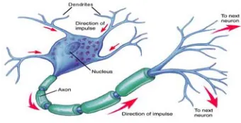
Artificial intelligence (AI) Systems are widely accepted as a technology offering an alternative way to tackle complex and ill-defined problems[13]. They can learn from examples, are fault tolerant in the sense that they are able to handle noisy and incomplete data, are able to deal with nonlinear problems, and once trained can perform prediction and generalization at high speed, They have been used in diverse applications in control, robotics, pattern recognition, forecasting, medicine, power systems, manufacturing, optimization, signal processing, and social/psychological sciences AI systems comprise areas like, expert systems, artificial neural networks, genetic algorithms, fuzzy logic and various hybrid systems, which combine two or more techniques[13]. Artificial Neural Network is a system loosely modeled on the human brain. A biological neuron is shown in (Fig. 2). In brain, there is a flow of coded information from the synapses towards the axon. The axon of each neuron transmits information to a number of other neurons. .According to Haykin a neural
[image:3.612.337.507.188.275.2]network is a massively parallel distributed processor that has a natural propensity for storing experiential knowledge and making it useful. It resembles the human brain in two respects: the knowledge is acquired by the network through a learning process, and inter neuron connection strengths known as synaptic weights are used to store the knowledge[13].
Fig. 2 :A simplified model of a biological neuron
A learning algorithm is defined as a procedure that consists of adjusting the weights and biases of a network, to minimize an error function between the network outputs, for a given set of inputs, and the correct outputs. ANNs have been widely used for many areas, such as control, data compression, forecasting, optimization, pattern recognition, classification, speech, vision, etc. Nowadays, ANNs have been trained to overcome the limitations of the conventional approaches to solve complex problems. ANNs can be trained to solve problems that are difficult for
supervised one, input is presented to the network along with the desired output and the weights are adjusted so that the network attempts to produce the desired output. The weights, after training, contain meaningful information whereas before training they are random and have no meaning. Neural networks that do not rely on the use of target data are trained using unsupervised learning. Instead of trying to map the data input–output relationship, the goal is to find an underlying structure of the data. There are different learning algorithms. A
popular algorithm is the back-propagation algorithm, which have different variants. Back-propagation
training algorithms gradient descent and gradient descent with momentum are often too slow for practical problems because they require small learning rates for stable learning. In addition, success in the algorithms depends on the user dependent parameters learning rate and momentum constant. Faster algorithms such as conjugate gradient, quasi-Newton, and Levenberg– Marquardt (LM) use standard numerical optimization techniques. These algorithms eliminate some of the disadvantages above mentioned. ANN with back-propagation algorithm learns by changing the weights, these changes are stored as knowledge. LM method is in fact an approximation of the Newton’smethod. The algorithm uses the second-order derivatives of the cost function so that a better convergence behavior can be obtained. In the ordinary gradient descent search, only the first order derivatives are evaluated and the parameter change information contains solely the direction along which the cost is minimized, whereas the Levenberg–Marquardt technique extracts a biter parameter change vector. Suppose that we have a function E(X) which needs to be minimized with respect to the parameter vector x. The error during the learning is called as root-mean squared (RMS) and defined as follows:
2 1 2 1 − =
∑
j j j o t pRMS (1)
In addition, absolute fraction of variance (R2) and mean absolute percentage error (MAPE) are defined as follows respectively:
(
)
− − =∑
∑
j j j j j o o t R 2 2 2 ) (1 (2)
100
×
−
=
o
t
o
[image:4.612.341.525.356.469.2]MAPE
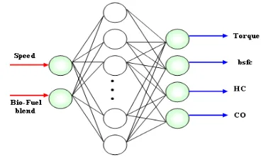
(3) Where t is target value, o is output value, and p is pattern. Input and output layer are normalized in the (-1,1) or (0,1) range. To get the best prediction by the network, several architectures were evaluated and trained using the experimental data. The back-propagation algorithm was utilized in training of all ANN models. This algorithm uses the supervised training technique where the network weights and biases are initialized randomly at the beginning of the training phase. The error minimization process is achieved using gradient descent rule. There were two input and four output parameters in the experimental tests. The two input variables are engine speed in rpm and the percentage of biodiesel blending with the conventional diesel fuel. The four outputs for evaluating engine performance are engine torque in Nm, Brake Specific Fuel Consumption (bsfc) in lit/KW hr, and emissions including HC and CO in ppm. Therefore the input layer consisted of 2 neurons which corresponded to engine speed and levels of biofuel blends and the output layer had 4 neurons (Fig. 3).Fig. 3: Configuration of multilayer neural network for predicting engine parameters
ANNs. The complexity and size of the network was also important, so the smaller ANNs had the priority to be selected. Finally, a regression analysis between the network response and the corresponding targets was performed to investigate the network response in more detail. Different training algorithms were also tested and finally Levenberg-Marquardt (trainlm) was selected. The computer program MATLAB 7.2, neural network toolbox was used for ANN design.
RESULTS AND DISCUSSIONS
Fuels Properties: Transesterification of the waste
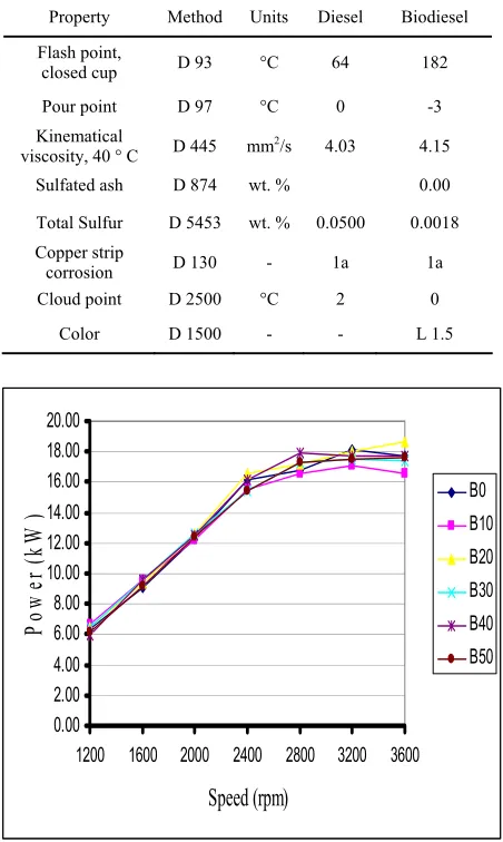
vegetable oil reduced the viscosity from 31.8 mm2/s to 4.15 mm2/s. This achievement paved the way to use the produced biofuel to be used as diesel engine fuel without any engine modifications. The biodiesel high flash point makes it possible for its easy storage and transportation. It should be noted that the diesel fuel flashpoint is 64◦C. The biodiesel sulfur content is another interesting advantage of the produced fuel which is 18 ppm only. Comparing the 18 ppm sulfur content of the produced biodiesel with the 500 ppm sulfur content of the diesel fuel used in Tehran operating diesel vehicles, the advantage of the biodiesel over the diesel fuel in terms of the environmental benefits can be justified. This comparison indicates that the sulfur content of biodiesel produced from the waste vegetable oil in Iran is 28 times lesser than the diesel fuels used in Tehran diesel vehicles. An easy way of reducing the diesel fuel sulfur content is the biodiesel blend which is the subject matter of an ongoing research work; its result may be published in near future. Fuel properties are mentioned in Table 3.
Torque and Power: First of all, fuel rack is placed in
[image:5.612.316.542.106.484.2]maximum fuel injection position for full load conditions. Then, the engine is loaded slowly. The engine speed is reduced in this way with increasing load. The trend of performance curves (power and torque) are very common like those mentioned in valid concerned literature. Range of speed was selected between 1200 – 3600 rpm. Engine test results with net diesel fuel showed that maximum torque was 64.2 Nm which occurred at 2400 rpm. The maximum power was 18.12 kW at 3200 rpm. Power and torque for fuel blends at full load is shown in figs. 4 and 5. Considering power and torque performance with fuel blends, one can say that the trend of these parameters versus speed is perfectly similar to net diesel fuel. Fig. 4 and Table 4 show engine speed and engine power relationship at full load condition using net diesel fuel and fuel blends. The net diesel fuel is used as a base for comparison. The fuel blend behavior is similar to that of net diesel fuel in developing power.
Table 3: Fuel properties
Property Method Units Diesel Biodiesel
Flash point,
closed cup D 93 °C 64 182
Pour point D 97 °C 0 -3
Kinematical
viscosity, 40 ° C D 445 mm2/s 4.03 4.15
Sulfated ash D 874 wt. % 0.00
Total Sulfur D 5453 wt. % 0.0500 0.0018
Copper strip
corrosion D 130 - 1a 1a
Cloud point D 2500 °C 2 0
Color D 1500 - - L 1.5
0.00 2.00 4.00 6.00 8.00 10.00 12.00 14.00 16.00 18.00 20.00
1200 1600 2000 2400 2800 3200 3600
Speed (rpm)
Po
w
er
(
kW
)
B0B10B20 B30 B40 B50
Fig. 4: Relationship between engine speed and engine power for different fuel blends
[image:5.612.318.534.574.692.2]Fig. 5 and Table 5 show engine torque for all fuels used at full load condition.
Table 4: Engine power at full load using diesel and fuel blends
0 10 20 30 40 50 60 70
1200 1600 2000 2400 2800 3200 3600
Speed (rpm)
T
or
que
(
N
m
) B0
[image:6.612.74.296.94.269.2]B10 B20 B30 B40 B50
[image:6.612.317.541.96.265.2]Fig. 5: Relationship between engine speed and torque for different fuel blends
Table 5: Engine torque at full load using diesel and fuel blends
B0 B10 B20 B30 B40 B50
50.2 53.1 51.2 51.2 47.1 49.1 54.1 57.1 56.1 57.4 57.1 54.9 58.8 58.4 60.1 60.4 59.6 59.1 64.2 61.6 66.1 61.2 64.1 61.4 57.1 56.6 58.7 59.1 61.2 59.1 54.1 50.9 53.9 52.1 53 52.1 47.1 43.9 49.4 46.1 47 46.8 55.086 54.514 56.500 55.357 55.586 54.643
Fuel consumption: Fuel consumption curves of net
diesel fuel at full load are shown in fig. 6. The curves show that fuel consumption at full load condition and low speeds is high. Fuel consumption first decreases and then increases with increasing speed. The reason is that, the produced power in low speeds is low and the main part of fuel is consumed to overcome the engine friction. Irrespective of fuel consumption at low speed (1200 rpm), fuel consumption is increased with increasing speed. The reason probably is that, friction power increases with increasing speed. Fig. 6 and Table 6 show brake specific fuel consumption with various fuels blend percentage. The curves show that brake specific fuel consumption of fuel blends trends is very similar to net diesel fuel. Brake specific fuel consumption of fuel blends is higher than net diesel fuel. In other words, increasing fuel blend percentage, a mild increase in brake specific fuel consumption is observed.
0.0000 0.0500 0.1000 0.1500 0.2000 0.2500 0.3000 0.3500 0.4000 0.4500 0.5000
1200 1600 2000 2400 2800 3200 3600
Speed (rpm)
sf
c(
lit
er
/k
W
hr
) B0
B10 B20 B30 B40 B50
Fig. 6: Effect of fuel blends on bsfc at full load and different speeds
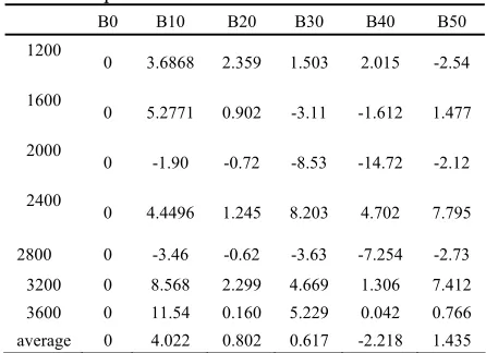
Table 6 shows increased engine brake specific fuel consumption in comparison with net diesel fuel at full load condition and various speeds. This table shows that mean value of engine specific fuel consumption of 10, 20, 30, 40 and 50% blends for various engine speeds is 4.0, 0.8, 0.6, -2.2 and 1.4 percent respectively higher than net diesel fuel.
Exhaust emission: Biodiesel contains oxygen in its
[image:6.612.73.292.314.443.2]structure. When biodiesel is added to diesel fuel, the oxygen content of fuel blend is increased and thus smaller oxygen is needed for combustion. However oxygen content of fuel is main reason for better combustion and CO and HC emission reduction, (figs. 7 and 8).
Table 6: Variation of bsfc using fuel blends with respect to diesel fuel
B0 B10 B20 B30 B40 B50 1200
0 3.6868 2.359 1.503 2.015 -2.54
1600
0 5.2771 0.902 -3.11 -1.612 1.477
2000
0 -1.90 -0.72 -8.53 -14.72 -2.12
2400
0 4.4496 1.245 8.203 4.702 7.795
2800 0 -3.46 -0.62 -3.63 -7.254 -2.73
[image:6.612.315.538.531.693.2]0.000 0.100 0.200 0.300 0.400 0.500 0.600
B0 B10 B20 B30 B40 B50
Fuel type
%C
[image:7.612.74.300.95.237.2]O
Fig. 7: Effect of fuel blends on average CO emission at full load
0.000 5.000 10.000 15.000 20.000 25.000 30.000 35.000
B0 B10 B20 B30 B40 B50
Fuel type
H
C
(
ppm
)
Fig. 8: Effect of fuel blends on average HC emission at full load
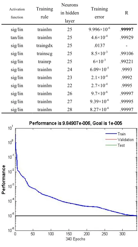
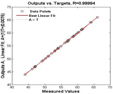
A network with one hidden layer and 25 neurons proved to be an optimum ANN as shown in Table 7. R in Table 7 represents the correlation coefficient (R-value) between the outputs and targets. The R-value didn't increase beyond 25 neurons in the hidden layer. Consequently the network with 25 neurons in the hidden layer would be considered satisfactory. The initial weights and bias were 1.3562, -3.7591 and 19.433, respectively in the first layer. The performance of the network in training is shown in fig. 9. The goal for the training was set to 10-5. This ensured a satisfactory response. From all the networks trained, few ones could provide this condition, from which the simplest network was chosen. To have a more precise investigation into the model, a regression analysis of outputs and desired targets was performed as shown in (figs. 9 to 13). There is a high correlation between the predicted values by the ANN model and the measured values resulted from experimental tests. The correlation coefficient was 0.99994 in the analysis of the whole network (Fig. 11), which implies that the model succeeded in prediction of the engine performance.
Table 7: Summary of different networks evaluated to yield the criteria of network performance
R Training
error Neurons
in hidden layer Training
rule
Activation
function
.99997
9.996×10⁻⁶
25 trainlm sig/lin
.99929 4.6×10⁻⁴
25 trainlm tan/lin
- .0137
25 traingdx sig/lin
.99106 8.5×10⁻³
25 trainscg sig/lin
.99221
6×10⁻³
25 trainrp
sig/lin
.9993 6.09×10⁻⁵
24 trainlm sig/lin
.9992 2.1×10⁻⁴
23 trainlm sig/lin
.9995 2.7×10⁻⁴
22 trainlm sig/lin
.99997 9.7×10⁻⁶
26 trainlm sig/lin
.99995 9.39×10⁻⁶
27 trainlm sig/lin
.99997 8.27×10⁻⁶
[image:7.612.315.539.119.520.2]28 trainlm sig/lin
Fig. 9: Training error (MSE) curve
[image:7.612.75.299.271.408.2]Fig. 10: regression analysis between the network response and the corresponding outputs
Fig. 11: The predicted outputs vs. the measured values of engine torque
Fig. 12: The predicted outputs vs. the measured values of bsfc
(a)
(b)
Fig. 13: The predicted outputs vs. the measured values, (a) CO (b) HC
REFRENCES
1. Ma, F., Hanna, M. A. 1999. Biodiesel production: a review. Bioresource technology, 70: 1-15.
2. Schumacher, L. G., Peterson, C. L. and Grepen, J. V. 2001. Fuelling direct diesel engines with 2 % biodiesel blend. Written for presentation at the 2001 annual international meeting sponsored by ASAE.
3. Ghobadian, B. and Rahimi, H. 2004. Biofuels-past, present and future perspective. International Iran and Russian congress of agricultural and natural science. Shahre cord university. Shahre cord. Iran. 4. Fukuda, H., Kondo, A. and Noda, H. 2001.
Biodiesel fuel production by transesterification of oils. Bioscience and bioengineering, 92: 405-416. 5. Anonymous 2003, European bioenergy networks.
[image:8.612.82.292.302.688.2]6. Lee, S. W., Herage, T., and Young, B. 2004. Emission reduction potential from the combustion of soy methyl ester fuel blended with petroleum distillate fuel. Fuel, 83: 1607-1613.
7. Wibulswas, P. 1999. Combustion of blend between plant oil and diesel oil. Renewable energy (on-line), 16: 1097 – 1101.
8. Al-Widyan, M. I. and Al-Shyoukh, A. O. 2002. Experimental evaluation of the transesterification of waste palm oil into biodiesel. Bioresource technology, 85: 253-256.
9. Bickel, K. and Strebig, K. 2000. Soy-Based diesel fuel study. University of Minnesota (diesel research).
10. Chou, J., McLeod D., Pozar M., Yee J. and Yeung A. 2003. UBC biodiesel initiative: helping communities to help their future. UBC seeds development studies.
11. Leung, D. Y. C. and Koo, B. C. P. 2000. Biodiesel – Is It Feasible To Be Used In Hong Kong? Vehicle exhausts treatment technology and control, 133-138.
12. Hertz, J., Krogh, A., Palmer, R. G. 1991. Introduction to the Theory of Neural Computation. Addison-Wesley Publishing Company, Redwood City, NJ.