1st International Conference on Modern Design, Construction and Maintenance of Structures, 10-11 December 2007, Hanoi, Vietnam
Analysis of laminated composite plate/shell structures using a stabilized
nodal- integrated quadrilateral element
*H. Nguyen-Van1, N. Mai-Duy1, T. Tran-Cong1
(1. CERSC, Faculty of Engineering and Surveying, The University of Southern Queensland, Toowoomba, Australia)
Abstract: A new simple and accurate four-node quadrilateral element is developed for linear static and dynamic analysis of thin to moderately thick laminated, anisotropic plate/shell structures within the first-order shear deformation theory (FSDT). The element is built by incorporating the strain smoothing method of mesh-free conforming nodal integration into the conventional bilinear four-node quadrilateral finite element (Q4). The membrane and bending stiffness matrices are calculated on the boundaries of the smoothing cells while the shear term is evaluated by 2×2 Gaussian quadrature. This boundary integration, which is done on the smoothing element boundaries for the bending and membrane term, contributes to the preservation of high accuracy of the method even when elements are extremely distorted, for example, when two nodes are collapsed so that the quadrilateral becomes a triangle. Through several structural analysis examples, the simplicity, efficiency and reliability of the element are demonstrated. Convergence and comparison studies with the other existing solutions in the literature suggest that the present element is robust, computationally inexpensive, free of locking and could be the simplest displacement type element of its class. Its convergence properties are insensitive to mesh distortion, thickness-to-span ratio, stacking sequence and degree of anisotropy.
Keywords: laminated composite plates; shells; strain smoothing method; shear-locking free; FSDT.
1 Introduction
Fibre-reinforced composite materials are ideal for many engineering applications that require high strength-to-weight, stiffness-to-weight ratios, excellent resistance to corrosive substances and potentially high overall durability. In recent years, the use of laminated composite plates/shells in many engineering applications has been expanding rapidly. This has led to more interesting researches on the development of simple and efficient elements for modelling of these structures. Many theories were developed for analysis of thin to thick laminated plates/shells such as the classical plate theory (CPT), the first-order shear deformation theory (FSDT), the higher-order shear deformation theory (HSDT), the layer-wise theory and 3D elasticity theory. Among these theories, the FSDT is still the most attractive approach owing to its simplicity, low computational cost and good compromise between numerical accuracy and computational burden.
A major problem of FSDT is the presence of shear-locking as the thickness-to-span ratio of the plate becomes too small (e.g. h/a<1/100). Many techniques have been proposed to overcome this phenomenon with varying degree of success. For instance, the reduced or selective integration methods [1], the hybrid/mixed methods [8], the assumed or modified shear strain technique [6], and the Timoshenko beam function approach [12]. However, the elements developed in these studies are usually stiff and sensitive to mesh distortion. It is rather difficult to obtain accurate results in several situations, including extremely distorted elements, coupling effects in non-symmetric laminates, and materials combination with high E1 to E2 ratio.
To avoid problems related to element distortion encountered in finite element method (FEM), many useful techniques of mesh-free method have been recently developed. For example, the stabilized conforming nodal integration (SCNI) is used as normalized nodal integration of the mesh-free Galerkin weak form [2, 3]. Although mesh-free method has good accuracy and high convergence rate, the complex approximation space increases the computational cost for numerical integrations. Recently, the application of SCNI in existing FEM for 2D elasticity problems was presented by Liu et al. [4, 5] as a new smoothed finite element method (SFEM). It is found that the SFEM achieves more accurate results and higher convergence rate as compared with the corresponding non-smoothed FEM without increasing the computational cost.
The present study is a contribution to the development of a simple, accurate and locking-free 4-node element, within the framework of the FSDT, which is able to work well in highly distorted forms for analysis of laminated
*
H. Nguyen-Van, PhD student
composite plates/shells of different shapes. We will extend and develop the idea of SFEM and propose a new locking-free flat quadrilateral laminated plate element based on the SCNI. The present four-node 20-DOF element is obtained by incorporating the SCNI into the Bathe-Dvorkin assumed strain plate element [6]. The membrane and bending strain fields are approximated using strain smoothing technique of mesh-free method. The shear strains are approximated by an independent interpolation field in the natural coordinate system. With this novel combination, the proposed element is locking free without zero energy modes and is able to provide accurate result in cases of extremely distorted elements, for example, even when two nodes are collapsed so that the quadrilateral becomes a triangle.
The paper is outlined as follows. A review of the FSDT and finite element formulations are introduced in section 2. The description of strain smoothing stabilization for membrane strain, curvature fields and the assumed natural shear strain of the element are derived in section 3. Several numerical applications are investigated in section 4 to assess the performance of the proposed element. Finally, section 5 concludes the study.
2 Review of the FSDT and finite element formulations for laminated plates
The first-order shear deformation theory (FSDT) for laminated plates is an extension of the Reissner-Mindlin theory for homogeneous isotropic thick plates. In FSDT, the plate kinematics is governed by the mid-surface (x-y
plane) displacement u0 ,v0, w0 and the rotation θx, θy around y- and x-axis, respectively
x z y x u z y x
u( , , )= 0( , )+
θ
, v(x,y,z)=v0(x,y)+zθ
y,
w(x,y,z)=w0(x,y).
(1) The inplane strain vector εm=[ε
xε
yε
z]T can be rewritten asT x y y x y y x x T x y y x b
m +z =[u0, v0, u0, +v0, ] +z[
θ
,θ
,θ
, +θ
, ]=ε ε
ε (2)
and the transverse shear strain vector γ=[
γ
xzγ
yz]T isT y y x
x w w ]
[ − , − ,
=
θ
θ
γ . (3)
The stress-strain relationship with respect to the global x- and y-axis for the kth (k=1…n) lamina is expressed as
ε Q σ k xy y x k k xy y x k Q sym Q Q Q Q Q = ⎪ ⎭ ⎪ ⎬ ⎫ ⎪ ⎩ ⎪ ⎨ ⎧ ⎥ ⎥ ⎥ ⎦ ⎤ ⎢ ⎢ ⎢ ⎣ ⎡ = ⎪ ⎭ ⎪ ⎬ ⎫ ⎪ ⎩ ⎪ ⎨ ⎧ =
γ
ε
ε
τ
σ
σ
66 26 22 16 12 11 , (4) γ C τ k s yz xz k k yz xz k Q k Q k k Q k k Q k = ⎭ ⎬ ⎫ ⎩ ⎨ ⎧ ⎥ ⎦ ⎤ ⎢ ⎣ ⎡ = ⎭ ⎬ ⎫ ⎩ ⎨ ⎧=
τ
τ
*γ
γ
44 2 2 * 45 2 1 * 45 2 1 * 55 2 1 , (5)
where k12,k22 are shear correction factors (SCFs); Qijk, Qij*k are elastic constants of the kth lamina making an angle θk with the global x-axis, which are given as
T k k
ε
εQ T
T
Q = , Q*k =TγQ*kTγT, (6)
in which k k G E E E E ⎥ ⎥ ⎥ ⎦ ⎤ ⎢ ⎢ ⎢ ⎣ ⎡ − − − − = 12 21 12 2 21 12 1 21 21 12 2 12 21 12 1 0 0 0 ) 1 ( ) 1 ( 0 ) 1 ( ) 1 (
ν
ν
ν
ν
ν
ν
ν
ν
ν
ν
Q , k k G G ⎥ ⎦ ⎤ ⎢ ⎣ ⎡ = 23 13 * 0 0Q , (7)
⎥ ⎥ ⎥ ⎦ ⎤ ⎢ ⎢ ⎢ ⎣ ⎡ − − − = 2 2 2 2 2 2 2 2 s c cs cs cs c s cs s c ε
T , ⎥
⎦ ⎤ ⎢ ⎣ ⎡ − = c s s c γ
T , c=cos
θ
k, s=sinθ
k. (8)The stress and resultant constitutive relation of the laminated plate can be expressed as
p p b m
p C ε
ε ε D B B A M N σ = ⎭ ⎬ ⎫ ⎩ ⎨ ⎧ ⎥ ⎦ ⎤ ⎢ ⎣ ⎡ = ⎭ ⎬ ⎫ ⎩ ⎨ ⎧
= , (9)
γ C T 0 0 44 2 2 0 45 2 1 0 55 2 1 0 55 2 1 s yz xz k k y x C k C k k C k k C k Q Q = ⎭ ⎬ ⎫ ⎩ ⎨ ⎧ ⎥ ⎦ ⎤ ⎢ ⎣ ⎡ = ⎭ ⎬ ⎫ ⎩ ⎨ ⎧
=
γ
γ
. (10)where N is the membrane force vector, M is the bending moment vector and T is the transverse shear force vector;A is the extensional stiffness, B is the bending-extensional coupling stiffness, D is the bending stiffness and C0 is the shear stiffness.
∑
= = = = np i i i T yx N q
w v u 1 ] [ Nq
u
θ
θ
, (11)where np is the total number of nodes of the mesh, q is the displacement vector of the element and N is the shape function matrix. In the case of standard Q4 element, Ni =0.25(1+
ξ
iξ
)(1+η
iη
).The corresponding approximation of membrane, bending and shear strain of Eq. (2) and (3) can be expressed in the following form
q B q B B ε ε ε p b m b m
p ⎥ =
⎦ ⎤ ⎢ ⎣ ⎡ = ⎭ ⎬ ⎫ ⎩ ⎨ ⎧
= , γ Bsq
yz xz = ⎭ ⎬ ⎫ ⎩ ⎨ ⎧ =
γ
γ
, (12) with ⎥ ⎥ ⎥ ⎦ ⎤ ⎢ ⎢ ⎢ ⎣ ⎡ = 0 0 0 0 0 0 0 0 0 0 0 , , , , x i y i y i x i m N N N N B , ⎥ ⎥ ⎥ ⎦ ⎤ ⎢ ⎢ ⎢ ⎣ ⎡ = x i y i y i x i b N N N N , , , , 0 0 0 0 0 0 0 0 0 0 0B , ⎥
⎦ ⎤ ⎢ ⎣ ⎡ = i y i i x i s N N N N 0 0 0 0 0 0 , ,
B . (13)
Then the element stiffness matrix can be obtained as
∫
∫
Ω Ω Ω + Ω = + = e e d d Ts s sp p T p e s e mb
e K K B C B B C B
K 0
.
(14)
3 Strain smoothing approach for finite element method
3.1 Smoothed membrane and bending strain approximation
The membrane, bending strain at an arbitrary point xC are obtained by using following strain smoothing
operation Ω − Φ =
∫
Ω d C p C p C ) ( ) ( ) (~ε x ε x x x
(15)
where εp is the membrane-bending strains obtained from displacement compatibility conditions as given in Eq. (12).
C
Ω is the smoothing cell domain on which the smoothing operation is performed. Depending on the stability analysis, ΩC may be an entire element or part of an element [2-3] as shown in Fig. 1; Φ is a given smoothing
function that satisfies at least unity property and is defined as
⎩ ⎨ ⎧ Ω ∉ Ω ∈ = − Φ . 0 , 1 ) ( C C C C A x x x x (16)
where
∫
Ω
Ω =
C
d
AC is the area of the smoothing cell (or subcell).
Substituting Φ into Eq. (15) and applying the divergence theorem, one can get the smoothed membrane-bending strain as follows
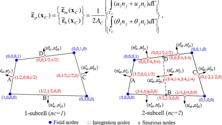
⎪ ⎪ ⎭ ⎪⎪ ⎬ ⎫ ⎪ ⎪ ⎩ ⎪⎪ ⎨ ⎧ Γ + Γ + = ⎭ ⎬ ⎫ ⎩ ⎨ ⎧ =
∫
∫
Γ Γ C C d n n d n u n uA i j j i
i j j i C C b C m C p ) ( ) ( 2 1 ) ( ~ ) ( ~ ) ( ~
θ
θ
x ε x ε x [image:3.595.122.477.545.745.2]ε , (17)
Fig. 1 Subdivision of smoothing cells (nc) and the values of shape function at nodes
Introducing the finite element approximation of u into Eq. (17) gives i T nc i C bi C mi i nc i C pi C
p x B x q B x B x q
ε ( ) ~ ( ) [~ ( ) ~ ( )]
~ 1 1
∑
∑
= = == , (18)
where nc is the number of smoothing cells (subcells) and
Γ ⎟ ⎟ ⎟ ⎠ ⎞ ⎜ ⎜ ⎜ ⎝ ⎛ =
∫
Γ d n N n N n N n N A C x i y i y i x i C C mi 0 0 0 0 0 0 0 0 0 0 0 1 ) ( ~ xB , Γ
⎟ ⎟ ⎟ ⎠ ⎞ ⎜ ⎜ ⎜ ⎝ ⎛ =
∫
Γ d n N n N n N n N A C x i y i y i x i C C bi 0 0 0 0 0 0 0 0 0 0 0 1 ) ( ~ xB . (19)
Using integration with one Gaussian point to evaluate Eq. (19) over each line segment ΓCi of ΓC, Eq. (19) can be transformed as
C b nb b x G b i y G b i y G b i x G b i C C mi l n N n N n N n N
A
∑
= ⎟⎟⎟⎟ ⎠ ⎞ ⎜⎜ ⎜ ⎜ ⎝ ⎛ = 1 0 0 0 ) ( ) ( 0 0 0 ) ( 0 0 0 0 0 ) ( 1 ) ( ~ x x x x x B , C b nb b x G b i y G b i y G b i x G b i C C bi l n N n N n N n N
A
∑
= ⎟⎟⎟⎟ ⎠ ⎞ ⎜⎜ ⎜ ⎜ ⎝ ⎛ = 1 ) ( ) ( 0 0 0 ) ( 0 0 0 0 0 ) ( 0 0 0 1 ) ( ~ x x x x x B . (20)
where xGb
,
lbC are the midpoint (Gaussian point) and the length of C bΓ , respectively and nb is the total number of edges of each smoothing cell.
3.2 Transverse shear strain approximation
The shear strain is approximated with independent interpolation fields in the natural coordinate system as [6]
⎥ ⎥ ⎥ ⎥ ⎥ ⎦ ⎤ ⎢ ⎢ ⎢ ⎢ ⎢ ⎣ ⎡ ⎥ ⎥ ⎥ ⎦ ⎤ ⎢ ⎢ ⎢ ⎣ ⎡ + − + − = ⎥ ⎦ ⎤ ⎢ ⎣ ⎡ = ⎥ ⎦ ⎤ ⎢ ⎣ ⎡ − − D C B A y x ξ η ξ η η ξ
γ
γ
γ
γ
η
η
ξ
ξ
γ
γ
γ
γ
) 1 ( 2 1 0 ) 1 ( 2 1 0 0 ) 1 ( 2 1 0 ) 1 ( 2 1 1 1 JJ , (21)
where J is the Jacobian matrix and the mideside nodes A, B, C, D are shown in Fig. 1. Expressing
γ
ηA,
Bξ
γ
,
Cη
γ
andD
ξ
γ
in terms of the discretized field u, we obtain the shear matrix⎥ ⎥ ⎦ ⎤ ⎢ ⎢ ⎣ ⎡ − − = − η η η ξ ξ ξ , 21 , 22 , , 11 , 12 , 1 0 0 0 0 i i i i i i i i i i si N b N b N N b N b N J
B , (22)
where bi11 =
ξ
ix,Mξ ; bi12 =ξ
iy,Mξ ; bi21 =η
ix,Lη; bi22 =η
iy,Lη,in which
ξ
i∈{−1,1,1,−1} ;η
i∈{−1,−1,1,1} and (i,M,L)∈{(1,B,A);(2,B,C);(3,D,C);(4,D,A)}.Finally, the element stiffness matrix can be obtained as follows
Ω + = + =
∑
∫
= Ω nc C s s T s C pC p T pC e s e mb e e d A 1 ~ ~ ~ ~ B C B B C B K KK . (23)
In Eq. (23), the shear term Kes is still evaluated by 2x2 Gauss quadrature while the membrane-bending stiffness
e mb
K~ is computed by one Gaussian point along each line segment of the smoothing cells of the element. For simplicity, two smoothing cells (nc= 2) as shown in Fig. 1 are used for calculating the smoothed membrane-bending stiffness matrix of the element. This forms the basis of a new four-node quadrilateral element named MISQ20 (Mixed Interpolation Smoothing Quadrilateral element with 20 DOF) for analysis of laminated plates. For analysis of laminated shells with MISQ20 element, one drilling degree of freedom will be added to each node of MISQ20 element for modelling and the total DOFs will be 24.
4 Numerical examples
4.1 Example 1: Simply supported cross-ply laminated plates under uniformly distributed load
The symmetric [0/90/0] and unsymmetric [0/90] cross-ply laminated square plates with a length a and a thickness h, subjected to simply supported boundary, under a uniform transverse load qo=1 are studied. All layers have
The SCFs are assumed to be 5/6. Owing to symmetry, only a quarter of the plate is discretized using 3×3, 6×6, 12×12 meshes with regular as well as highly distorted elements as shown in Fig. 2.
Fig. 2 Example 1: Discretization of a plate quadrant with regular and irregular meshes.
Tab. 1 shows the prediction accuracies and convergence rate for the dimensionless plate centre deflections
w*=100E2wh 3
/(qoa 4
) with two types of meshes. It is found that the accuracy of the present element is better than EML4 element [7], HASL element [8] for the case of regular mesh 12×12. Numerical results in Tab. 1 also indicate that element performance, in terms of rate of convergence and accuracy, with respect to exact solution is excellent. The proposed MISQ20 element yields not only accurate results in a wide range of thick to thin plates but also rapid convergence for both regular and extremely distorted meshes.
Tab. 1 Example 1: Convergence of normalized central deflection w*=100E2wh3 /(qoa4)and comparison with other solutions.
MISQ20
h/a Lay-up Mesh EML4
12×12
HASL
12×12 3×3 6×6 12×12 Exact
0.001 Regular − − 1.6897 1.6943 1.6952 −
Irregular − − 1.6813 1.6918 1.6947
0.01 [0/90] Regular − − 1.6923 1.6967 1.6979 1.6980
Irregular − − 1.6862 1.6928 1.6973
0.1 Regular 1.9470 − 1.9465 1.9469 1.9469 1.9468
Irregular − − 1.9516 1.9478 1.9466
0.001 Regular − − 0.6736 0.6676 0.6664 −
Irregular − − 0.6728 0.6676 0.6667
0.01 [0/90/0] Regular − 0.6700 0.6773 0.6713 0.6700 0.6697
Irregular − − 0.7006 0.6736 0.6702
0.1 Regular 1.0220 1.0262 1.0367 1.0254 1.0227 1.0219
Irregular − − 1.0735 1.0312 1.0232
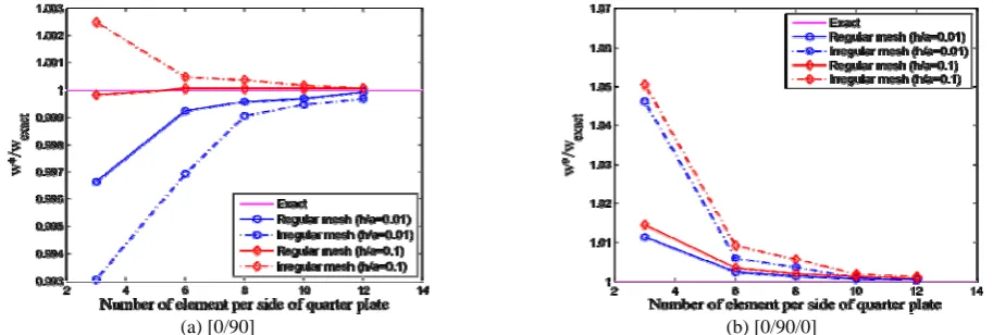
The effect of distorted mesh and thickness ratio h/a on the convergence of the results is shown in Fig. 3. It is found that the convergence of the solution w* for unsymmetric cross-ply [0/90] with h/a=0.1 is faster than with
h/a=0.01 in both types of mesh and conversely for symmetric cross-ply [0/90/0].
[image:5.595.70.527.545.699.2](a) [0/90] (b) [0/90/0]
Fig. 3 Example 1: Convergence behavior of the normalized central deflection of unsymmetric and symmetric laminated plates.
4.2 Example 2: Simply supported angle-ply laminated plates under uniformly distributed load
A simply supported two-layer angle-ply [θ/-θ] square plate with length a =10 and thickness h = 0.02, subjected to a uniformly distributed transverse load qo = 1 is analyzed. The SCFs are 5/6. All layers have equal thickness and are
made of the same material: E1/E2=25, G12= G13 = 0.5E2 , G23= 0.2E2, υ12 = υ13 = υ23 = 0.25. Due to asymmetry, the
(a) (b)
Fig. 4 Example 2: (a) Geometry data and representative mesh; (b) Effect of fibre angle on accuracy.
Table 2 presents a convergence study of the normalized central deflection w*= 100E2wh3 /(qoa4) with different
fibre orientation angles. The present results are compared with other solutions obtained using MQH3T element [9], SQUAD4 element [10], RDTMLC element [11], RDKQ-L20 element [12] and the exact solution given by Whitney [13]. The effect of fibre orientation on the accuracy of the methods is also shown in Fig 2b. It can be seen that the accuracy of the present element compares very favourably with other elements and the method is convergent with mesh refinement as shown in Tab. 2. The accuracy obtained with the present MISQ20 element is quite insensitive with fibre angles while other methods behave badly in some cases.
Tab. 2 Example 2: Convergence of normalized central deflection with various fibre angles and comparison with other solutions.
MISQ20 Fibre
angle
MQH3T 6×6 (655DOF)
SQUAD4 10×10 (605DOF)
RDTMLC 8×8 (605DOF)
RDKQ-L20 10×10 (605DOF)
6×6 8×8 10×10 (605DOF)
Exact
±5 0.4764 0.4776 0.4776 0.4742 0.4793 0.4758 0.4748 0.4736
±15 0.7160 − 0.7014 0.7139 0.7191 0.7164 0.7155 0.7142
±25 0.7870 0.8030 0.7638 0.7854 0.7901 0.7886 0.7880 0.7870 ±35 0.7555 0.7745 0.7329 0.7538 0.7581 0.7571 0.7567 0.7561 ±45 0.7315 0.7506 0.7106 0.7302 0.7340 0.7331 0.7327 0.7322
4.3 Example 3: Antisymmetric 2-layer and 8-layer angle-ply laminated plates under double sinusoidal load To assess the combined effect of normal bending-in-plane shear and extension-twisting moment coupling on the performance of the MISQ20 element, simply supported 2-layer [-45/45] and 8-layer [-45/45]4 square plates with
length a and thickness h subjected to doubly sinusoidal load q= qosin(x/a)sin(y/a) are analyzed. The SCFs and
material are the same as in the previous example (section 4.2).
The numerical results shown in Tab. 3 demonstrate the accuracy of the present method. Note that calculations are performed for the normalized central deflection w*=1000E2wh
3
/(qoa 4
); the normalized stress
σ
*x =σ
xh2/(qoa2)at point (a/2, a/2, h/2); the normalized shear stress
τ
xy* =τ
xyh2/(qoa2) at point (0, 0, -h/2); and the normalizedtransverse shear stress
τ
xz* =τ
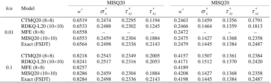
xzh/(qoa) at point (0, a/2, h/4).Tab. 3 Example 3: Comparison of normalized central deflection and normalized stresses with other solutions.
MISQ20 MISQ20
h/a Model
w*
σ
*xτ
*xyτ
*xz w*σ
*xτ
*xyτ
xz*CTMQ20 (8×8) 0.6519 0.2474 0.2295 0.1194 0.2463 0.1459 0.1356 0.1791
RDKQ-L20 (10×10) 0.6533 0.2488 0.2302 0.1245 0.2466 0.1464 0.1359 0.1813
0.01 MFE (8×8) 0.6558 − − − 0.2472 − − −
MISQ20 (10×10) 0.6553 0.2459 0.2304 0.1884 0.2475 0.1427 0.1368 0.2358
Exact (FSDT) 0.6564 0.2498 0.2336 0.2143 0.2479 0.1445 0.1384 0.2487
CTMQ20 (8×8) 0.8218 0.2543 0.2349 0.2005 0.4157 0.1507 0.1361 0.2384
RDKQ-L20 (10×10) 0.8241 0.2517 0.2316 0.2053 0.4171 0.1512 0.1370 0.2420
0.1 MFE (8×8) 0.8257 0.4189
MISQ20 (10×10) 0.8286 0.2459 0.2304 0.1884 0.4208 0.1427 0.1368 0.2358
Exact (FSDT) 0.8284 0.2498 0.2336 0.2143 0.4198 0.1445 0.1384 0.2487
4.4 Example 4: Free vibration of cross-ply laminated plates
A simply supported four-layer cross-ply [0/90/90/0] square laminate is studied with material properties: G12= G13
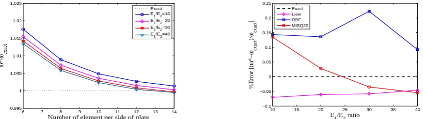
[image:6.595.61.536.586.733.2]element yields not only accurate results in a wide range of E1/E2 ratio but also rapid convergence as in Fig. 5a. The
effect of various modulus ratios of E1/E2 on the accuracy of the fundamental frequency is also displayed in Fig. 5b. It
can be seen that the present results are in good agreement with exact solution [16] and closer to Liew’s results [14] than RBF’s solution by Ferreira [15].
6 7 8 9 10 11 12 13 14
0.995 1 1.005 1.01 1.015 1.02 1.025
Number of element per side of plate
ω
*/
ωexact
Exact
E1/E2=10
E1/E2=20
E1/E2=30
E 1/E2=40
10 15 20 25 30 35 40
−0.1 −0.05 0 0.05 0.1 0.15 0.2 0.25
E
1/E2 ratio
%Error [(
ω
*−
ω exact
)/
ω exact
]
Exact Liew RBF MISQ20
Fig. 5 Example 4: Convergence study and effect of modulus ratios on the accuracy of the fundamental frequency.
To assess the effect of mesh distortion, the plate is analysed again using distorted elements. The coordinates of an irregular mesh are obtained by the following expressions: x’= x+Δx rc s and y’= y+Δy rc s; where rc is a
computer-generated random number between -1.0 and 1.0; Δx, Δy are initial regular element sizes in x- and y- directions, respectively and s∈ [0;0.4] is used to control the shape of the distorted element: the bigger the value of s, the more irregular the shape of generated elements.
s= 0 s= 0.2
s= 0.3 s= 0.4 0 0.05 0.1 0.15 0.2 0.25 0.3 0.35 0.4 −0.1
−0.05 0 0.05 0.1 0.15 0.2 0.25 0.3
Distorsion ratio s
% Error [(
ω
*−
ω exact
)/
ω exact
]
Exact
E1/E2=10
E1/E2=20
E1/E2=30
[image:7.595.80.517.116.239.2]E1/E2=40
Fig. 6 Example 4: The effect of mesh distortion on the accuracy of the present method.
The effect of the mesh distortion on the fundamental frequency obtained by the present method is shown in Fig. 6. It is noted that the accuracy of the fundamental frequencies associated with irregular mesh decreases in comparison with regular mesh results. However, the deterioration is very small and the overall performance is insensitive to mesh distortion as the maximum error of frequency is below than 0.3%.
4.5 Example 5: Free vibration of multi-layer cylindrical shells
A simply supported cross-ply cylindrical panels with R=100, L=20 and a total thickness h=0.2 as shown in Fig.7 is studied.
Fig. 7 Example 5: Finite element and geometry data of the cylindrical shell.
All layers have equal thickness and same material: E1/E2= 25, G12= G13= 0.5E2, G23= 0.2E2, υ12 = υ13 = υ13 =
Tab. 5 Example 5: Convergence of normalized fundamental frequencies with various layup and comparison with other solutions.
Layerwise [17] 9-node element [18] MISQ20 Analytic
Lay-up
8×8 5×5 4×4 6×6 8×8 [19]
[0/90] 17.390 17.7 17.061 16.833 16.736 16.668
[0/90/0] 20.960 − 20.575 20.340 20.240 20.332
[0/90/90/0] 20.960 − 20.694 20.461 20.367 20.361
5 Conclusions
An accurate simple four-node displacement-based quadrilateral element MISQ20 has been developed and reported in this paper for linear analysis of thin to thick laminated plates/shells. The element is based on mixed interpolations with a strain smoothing technique used in the SCNI mesh-free method and it is easy to implement. With this combination, the element maintains a sufficient rank and free from shear locking and any spurious modes. Several numerical examples are studied and the obtained results are in excellent agreement with analytical solution. It is found that the new proposed element is robust, reliable and is not sensitive to mesh distortion. It can yield accurate results even with coarse discretizations irrespective of the thickness-to-span ratio and stacking sequence.
References
[1] Hughes T, Cohen M, Haroun. Reduced and selective integration techniques in finite element analysis of plate [J].
Nuclear Engineering Design, 1978, 46: 203–222.
[2] Wang D, Chen J.S. Locking-free stabilized conforming nodal integration for meshfree Mindlin-Reissner plate formulation [J]. Computer Methods in Applied Mechanics and Engineering, 2004, 193: 1065–1083.
[3] Wang D, Dong S.B, Chen J.S. Extended meshfree analysis of transverse and inplane loading of a laminated anisotropic plate of general platform geometry [J]. International Journal of Solids and Structures, 2006, 43: 144– 171.
[4] Liu G. R, Dai K. Y, Nguyen T. T. A smoothed finite element method for mechanics problems [J]. Computational Mechnics, 2007, 39: 859–877.
[5] Liu G. R, Dai K. Y, Nguyen T. T. Theoretical aspects of the smoothed finite element method (SFEM) [J].
International Journal for Numerical Methods in Engineering, 2006, in press.
[6] Bathe K.J, Dvorkin E.N. A four node plate bending element based on Mindlin-Reissner plate theory and a mixed interpolation [J]. International Journal for Numerical Methods in Engineering, 1985, 21: 367–383.
[7] Auricchio F, Sacco E. A mixed-enhanced finite-element for the analysis of laminated composite plates [J].
International Journal for Numerical Methods in Engineering, 1999, 44: 1481–1504.
[8] Cazzani A, Garusi E, Tralli A., Atluri S. A four-node hybrid assumed-strain finite element for laminated composite plate [J]. CMC: Computers, Materials & Continua, 2005, 2: 23–38.
[9] Spilker RL, Jakobs DM, Engelmann BE. Efficient hybrid stress isoparametric elements for moderately thick and thin multiplayer plates [J]. Hybrid and Mixed Finite Element Method, 1985, 73: 113–122.
[10] Wilt TE, Saleeb AF, Chang.TY. Mixed element for laminated plates and shells [J]. Computers and Structures, 1990, 37: 597–611.
[11] Ge Z, Chen WJ. A refined discrete triangular Mindlin element for laminated composite plates [J]. Structural Engineering and Mechanics, 2002, 14: 575–579.
[12] Zhang YX, Kim K. S. Two simple and efficient displacement-based quadrilateral elements for the analysis of the composite laminated plates [J]. International Journal for Numerical Methods in Engineering 2004, 61: 1771–1796. [13] Whitney JM. Bending-extensional coupling in laminated plates under transverse load [J]. Journal of Composite
Materials, 1969, 3: 398–411.
[14] Liew K.M, Huang Y.Q, Reddy J.N. Vibration analysis of symmetrically laminated plates based on FSDT using the moving least squares differential quadrature method [J]. Computer Methods in Applied Mechanics and Engineering, 2003, 192: 2203–2222.
[15] Ferreira A.J.M, Roque C.M.C, Jorge R.M.N. Free vibration analysis of symmetric laminated composite plates by FSDT and radial basis functions [J]. Comput. Methods Appl. Mech. Engrg., 2005, 194: 4265–4278.
[16] Reddy J.N. Mechanics of laminated plates and shells-Theory and analysis [M]. CRC Press, 2004.
[17] Liu M.L, To C.W.S. Free vibration analysis of laminated composite shell structures using hybrid strain based layerwise finite elements [J]. Finite Elements in Analysis and Design, 2003, 40: 83–120.
[18] Jayasankar S, Mahesh S, Narayanan S, Padmanabhan C. Dynamic analysis of layered composite shells using nine node degenerate shell elements [J]. Journal of Sound and Vibration, 2007, 299: 1–11.
[19] Reddy J.N. Exact solutions of moderately thick laminated shells [J]. ASCE J. Eng. Mech, 1984, 110(4): 794–809