Detecting High-Dimensional Outliers: the
New Task, Algorithms and Performance
Ji Zhang
1, Hai Wang
21
Department of Computer Science, University of Toronto,
Toronto, Ontario, Canada, M5S 3G4
Email: [email protected]
2
Saint Mary’s University,
Halifax, Canada
Email: [email protected]
Abstract
Outlier detection is a fundamental step in knowledge discovery in databases. With the increasing number of high-dimensional databases, existing outlier detection algorithms that work only in the context of full space are unable to effectively screen out informative outliers. This is because majority of these outliers exists only in subspaces. In this paper, we identify a new outlier detection task for high-dimensional data, i.e. finding the subspaces in which given points are outliers, and propose a novel outlier detection algorithm, called High-D Outlier Detection (HighDOD). The intuitive idea is that we measure the outlying degree of the point using the sum of distances between this point and its k nearest neighbors. Two pruning strategies are proposed to realize fast pruning in the subspace search and an efficient dynamic subspace search method with a sample-based learning process has been implemented. Experimental results show that HighDOD is efficient and outperforms the naive top-down, bottom-up and random search methods.
1. Introduction
Outlier detection is an important step in data mining that enjoys a wide range of applications such as the detection of credit card frauds, criminal activities and exceptional patterns in databases. Outlier detection problem can typically be formulated as follows: given a set of data points or objects, find a specific number of objects that are considerably dissimilar, exceptional and inconsistent with respect to the remaining data [9].
of them only consider outliers in the entire space. This implies that they will miss out on the important information about the subspaces in which these outliers exist.
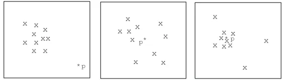
Consider the example in Figure 1. Three 2-dimensional views of the high-dimensional data are presented. Note that pointpexhibits different outlying degrees in these three views. In the leftmost view, p is clearly an outlier. However, this is not so in the other two views. Finding the correct subspaces so that outliers can be detected is critical to applications such as fraud detection.
x x x x
x
x x x x x
* p
x x
x x
x
x
x x
x x
* p
x x x
x x xx
x x
[image:2.595.164.448.189.269.2]x * p
Figure 1: 2-dimensional views of the high-dimensional data
A recent trend in high-dimensional outlier detection is to use evolutionary search method [4] where outliers are detected by searching for sparse subspaces. Points in these sparse subspaces are assumed to be the outliers. While knowing which data points are the outliers can be useful, in many applications, it is more important to identify the subspaces in which a given point is an outlier, which motivates the proposal of a new technique in this paper to handle this new outlier detection task. For example, in the case of designing a training program for an athlete, it is critical to identify the specific subspace(s) in which an athlete deviates from his or her teammates in the daily training performances. Knowing the specific weakness (subspace) allows a more targeted training program to be designed. In a medical system, it is useful for the Doctors to identify from voluminous medical data the subspaces in which a particular patient is found abnormal and therefore a corresponding medical treatment can be provided in a timely manner.
The major contribution of this paper is the proposal of a dynamic subspace search algorithm, called HighDOD, that utilizes a sample-based learning process to efficiently identify the subspaces in which a given point is an outlier. Note that, instead of detecting outliers in specific subspaces, our method searches for the associated subspaces whereby the given data points exhibit abnormal deviations. To our best knowledge, this is the first such work in the literature so far.
The main features of HighDOD include:
1. The outlying measure, OD, is based on the sum of distances between a data and its k nearest neighbors[2]. This measure is simple and independent of any underlying statistical and distribution characteristics of the data points.
2. Two heuristic pruning strategies are proposed to aid in the search for outlying sub-spaces.
4. The heuristic on the minimum sample size based on the hypothesis testing method is also presented.
The reminder of this paper is organized as follows. In Section 2, we present a survey of related work in outlier detection algorithms. Section 3 discusses the basic notions and prob-lem to be solved. In Section 4, we present our outlier detection technique, called HighDOD, in high-dimensional data. Section 5 discusses the detailed algorithms of HighDOD. Experi-mental results are reported in Section 6. In Section 7, a practical application of HighDOD is presented. Section 8 concludes this paper.
2. Related Work
An outlier is an observation that deviates so much from other observations so that it arouses suspicious that it is generated by a different mechanism [10]. Literatures on outlier detection algorithms have been abundant in recent years and can be classified into five major cate-gories based on the techniques used, i.e. distribution-based methods, depth-based methods, distance-based methods, density-based methods and clustering-based methods.
Distribution-based methods [5, 10] rely on the statistical approaches that assume a distribution or probability model to fit the dataset. Over one hundred discordancy/outlier tests have been developed for different circumstances, depending on the parameter of dataset (such as the assumed data distribution) and parameter of distribution (such as mean and variance), and the expected number of outliers [9, 13]. However, distribution-based meth-ods suffer from some key drawbacks. First, they cannot be applied in a multi-dimensional scenario because they are univariate in nature. In addition, the lack of any prior knowledge regarding the underlying distribution of the dataset makes the distribution-based methods difficult to use in practical applications. Finally, the quality of results cannot be guaranteed because they are largely depended on the distribution chosen to fit the data.
Another kind of outlier detection methods in statistics is the depth-based methods [17, 19]. Such methods organize the data in the form of layers in the data space and detect outliers mainly in the shallower layers. This idea is based on the observation that outliers are more likely to be the points with smaller depths, so the shallower the layers are, the more likely they are to contain outliers than the deeper layers. Yet, depth-based methods are only applicable in lower dimensional data due to the expensive computation of k-d convex hulls that has a low bound complexity of O(N k/2) for N objects.
[13] and [14] proposed the notion of distance-based outliers, i.e. DB(pct, dmin)-Outlier, which defines an object in a dataset as a DB(pct, dmin)-Outlier if at leastpct% of the objects in the datasets have the distance larger than dmin from this object. In other words, the cardinality of the points having distance smaller thandmin is no more than (100−pct)% of the size of dataset. In [18], the notion of distance-based outlier is extended and the distance to the kth nearest neighbors of a point p, denoted asDk(p), is proposed to rank the point so
Recently, a density-based formulation scheme of outlier has been proposed in [7]. This formulation ranks the outlying degree of the points using Local Outlier Factor (LOF). LOF of an object intuitively reflects the density contrast between its density and those of its neighborhood. Note that LOF ranks points by only considering the neighborhood density of the points, thus it may miss the potential outliers whose densities are close to those of their neighbors. [12] improves the efficiency of algorithm in [7] by proposing an efficient micro-cluster-based local outlier mining algorithm, but it still use LOF to mine outliers in dataset.
The final category of outlier detection algorithm is clustering-based. So far, they are numerous studies on the clustering and a number of them are equipped with some mecha-nisms to detect outliers, such as CLARANS [16], DBSCAN [8], BIRCH [21], WaveCluster [20], DenClue[11] and CLIQUE[1]. Strictly speaking, clustering algorithms should not be considered as outlier detection methods, because their objective is only to group the objects in dataset such that clustering functions can be optimized. The aim to eliminate outliers in dataset using clustering is only to dampen their adverse effect on the final clustering result. The methods discussed in the aforementioned four categories are not sufficiently ap-plicable to high-dimensional data. All of them try to define outliers based on the distance in full dimensional space in one way or another [4]. But in high-dimensional scenario, the data points are not likely to exhibits noticeable abnormal behaviors and this abnormality will show in some lower subspaces of full dimensionality. [4] is the first work identifying this problem in high-dimensional outlier detection and tries to solve this problem by searching sparse subspace using evolutionary search method. The evolutionary search method works by first finding all the lower dimensional projections that are locally sparse. The sparsity of a
k-dimensional projection is measured by the so-called Sparse Coefficient of the corresponding
k-dimensional cube. Formally, let n(D) be the number of points in the k-dimensional data cube and each attribute of the data is divided into φ equip-depth ranges and let f = 1/φ. The sparsity coefficient S(D) of the cube D is calculated as S(D) = √n(D)−N fk
N fk
(1−fk
). However,
this Sparse Coefficient is not characterized by any upward or downward closure in the set of dimensions, hence, no pruning mechanism can be performed to find the sparse subspaces quickly.
Remarks: All the existing outlier detection, regardless of in low or high dimensional
sce-nario, invariably fall into the framework of detecting outliers in a specific data space, either in full space or subspace. We term these methods as ”space → outliers” techniques. For instance, [4] detects outliers by first finding locally sparse subspaces, and [14] discoveries the so-called Strongest/Weak Outliers by first finding the Strongest Outlying Spaces. Our technique is novel in that it approaches the problem of outlier detection from a different prospective: finding associate subspaces for each point in which this point is regarded as an outlier, which we can call it an ”outlier → spaces” technique.
3. Notations and Problem Formulation
Symbol Description
N Total number of data in the dataset
d Number of dimension of the dataset
k Number of nearest neighbors
T or Ts Distance threshold used
Nq Number of query points
[image:5.595.178.434.70.179.2]S Number of sampling points
Table 1: Notations used in the paper
3.1 Outlying Degree OD
For each point, we define the degree to which the point differs from the majority of the other points in the same space, termed the outlying degree (OD in short). OD is defined as the sum of the distances between a point and its k nearest neighbors in a data space[2]. Mathematically speaking, the OD of a point pin space s is computed as:
ODs(p) = k
X
i=1
Dist(p, pi)|pi ∈KN N Set(p, s)
where KN N Set(p, s) denotes the set composed by the k nearest neighbors of p in s. Note that the outlying degree measure is applicable to both numeric and nominal data: for nu-meric data we use Euclidean distance while for nominal data we use Hamming distance. Mathematically, the Euclidean distance between two numeric points p1 and p2 is defined
as Dist(p1, p2) = [P((p1i −p2i)/(M axi −M ini))2]1/2, where M axi and M ini denote the
maximum and minimum data value of the ith dimension. The Hamming distance between
two nominal pointsp1 and p2 are defined as Dist(p1, p2) =P|p1i−p2i|, where |p1i−p2i| is
0 if p1i equals to p2i and is 1 otherwise.
3.2 Problem Formulation
Recall our motivation is to find the subspaces in which a given point shows noticeable deviation from its neighboring points. A distance threshold T is utilized to decide whether or not a data point deviates significantly from its neighboring points.
We now formulate the new high-dimensional outlier detection problem as following: given a data point or object, find the subspaces in which this data is considerably dissimilar, exceptional or inconsistent with respect to the remaining points or objects.
This problem can be mathematically stated as: for any given point p, find the set of subspaces ϕ such that for each subspace s ∈ ϕ, we have ODs(p) ≥ T. If the answer set is
empty forp, we say that p is not an outlier in any subspaces.
Dynamic Subspace Searching
Detected Subspaces of Query Data
Users
Query Data
High-dimensional Dataset
Indexed High-dimensional data Sampled Data
Downward and upward pruning possibilities X-tree
Indexing
Dynamic Subspace Searching Random
[image:6.595.166.447.69.245.2]Sampling
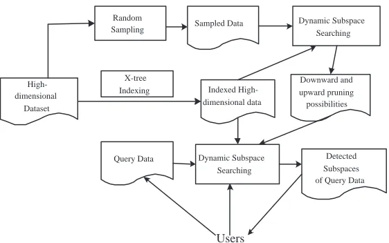
Figure 2: The overview of HighDoD
4. High-Dimension Outlier Detection
In the section, we present an overview of our High-Dimension Outlier Detection (HighDOD) method. Figure 2 shows an overview of the system. It mainly consists of three modules. The X-tree Indexing module performs X-tree [6] indexing of the high-dimensional dataset to facilitate kNN search in every subspace. Sample-based Learning module randomly samples the dataset and performs dynamic subspace search to estimate the downward and upward pruning probabilities of subspaces from 1 to d dimensions. Subspace Outlier Detection module uses the probabilities obtained in the Learning module to carry out a dynamic subspace search to find all the subspaces in which the given query data point is an outlier.
4.1 X-tree Indexing Module
We utilize X-tree (eXtended node tree) [6] to index the high-dimensional dataset in order to speedup the k-NN queries in different subspaces. It is an index structure that is designed to support efficient query processing of high-dimensional data. The introduction of X-tree is motivated by the problem with the R-tree-based index structures that the overlap of bounding boxes in the directory will increase as the dimension grows. The basic idea of X-tree is to use overlap-minimizing split and supernodes to keep the directory as hierarchical as possible and at the same time to avoid splits that will result in high overlap. It is a hybrid of linear array-like and R-tree like directory. The hierarchical organization is good for low dimensions, while in high dimensions, a linear organization is more efficient. Interested reader can refer to [6] for details on X-tree.
4.2 Subspace Pruning
In our work, we have utilized two classes of strategies for subspace pruning in the searching process, i.e. global-T pruning and local-T pruning. In the global-T pruning, a global distance threshold T is used for delimiting outlying and non-outlying subspaces in the whole lattice for a given data point. While in the local-T pruning, different distance thresholds are used for different subspaces required to evaluate in the searching process. Also, the subspace searching process can be performed either in an upward or a downward manner.
Global-T Pruning Strategy
OD maintains two interesting monotonic properties that allow the design of an effi-ciency outlier subspace search algorithm.
Property 1: If a pointp is not an outlier in a subspace s, then it cannot be an outlier in any
subspace that is a subset of s.
Property 2: If a point p is an outlier in a subspace s, then it will be an outlier in any subspace
that is a superset of s.
The above properties are based on the fact that the OD value of a point in a subspace cannot be less than that in its subset spaces. Mathematically, we have ODs1(p)≥ODs2(p)
if s1 ⊇s2.
Proof: Letak andbk be thekth nearest neighbors ofp in the anm-dimensional subspace s1
and n-dimensional subspaces s2, respectively (1≤ n ≤m ≤d and s1 ⊇s2). M axDists2(p)
is the maximum distance between p and ai, 1≤i≤k, in the subspace s2.
We haveDists1(p, ak)≥Dists1(p, ai)|1≤i≤k. Since s1 is a superset of s2, we thus know
Dists1(p, ai)≥Dists2(p, ai)|1≤i≤k. This impliesDists1(p, ak)≥Dists2(p, ai)|1≤i≤k, By
defini-tion of M axDists2, we have Dists1(p, ak) ≥M axDists2(p)≥Dists2(p, bk). In other words,
Dists1(p, ak) ≥ Dists2(p, bk). Likewise, it is hold that Dists1(p, ai) ≥ Dists2(p, bi)|1≤i≤k,
Since ODs1(p) =Pk1Dists1(p, ai) and ODs2(p) = Pk1Dists2(p, bi). We therefore conclude:
ODs1(p)≥ODs2(p).
In the downward global-T pruning strategy, we make use of Property 1 of OD to quickly prune away those subspaces in which the point cannot be an outlier. This is because
if ODs1(p)< T, then ODs2(p) < T, where s1 ⊇ s2 and T is the distance threshold. In the
upward global-T pruning strategy, Property 2 of OD is utilized to detect those subspaces in which the point is definitely an outlier. The reason is that ifODs2(p)≥T, thenODs1(p)≥T.
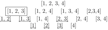
Consider a 4-dimensional dataset example as shown in Figure 3. Suppose we have determined that point p is not an outlier in subspace [1, 2, 3], then all the subspaces that are subset of [1, 2, 3], i.e. [1, 2], [1, 3], [2, 3], [1], [2] and [3], can be pruned by the downward pruning strategy. These subspaces are highlighted in Figure 3. On the other hand, if p is found to be an outlier in the subspace [1,4] (see Figure 4), then all the superset of [1,4], namely [1, 2, 3, 4], [1, 2, 4] and [1, 3, 4], are pruned by the upward pruning strategy.
The global distance thresholdT is specified as follows:
T =C√d· 1
d
d
X
i=1
where ODsi denotes the average OD values of points in the 1-dimensional subspace si and C is a constant factor. This specification stipulates that only those points whose OD values are significantly larger than the average level are regarded as outliers in the full space (the significance is specified by the constant factor C, normally we may setC=2 or 3).
Local-T Pruning Strategy
Let Ts be the distance threshold for subspace s and we have two space s1 and s2
satisfying s1 ⊇s2. In the downward local-T pruning strategy, if ODs1(p)< Ts1, then s2 will
be pruned only when the following requirement is satisfied:
∀si, ODsi(p)<
1
C ·ODsi|dim(si) = 1, si ⊆s1−s2
In the upward local-T pruning strategy, ifODs2(p)≥Ts2, thens1 will be pruned only
when the following requirement is satisfied:
∀si, ODsi(p)≥C·ODsi|dim(si) = 1, si ⊆s1−s2
whereC is the same constant factor used in the Global-T pruning. Being more conservative than the Global-T pruning, the above two requirements intuitively mean that the subspace s′
which is a superset/subset of the current subspaces can be pruned only when the OD(p) value in each of the 1-dimensional subspaces that belong to the difference of the two subspaces (i.e. s′ −s) is significantly larger or smaller than the corresponding average level.
Similar to the specification of the global distance threshold T, we can specify Ts, the
distance threshold for a m-dimensional subspace s, 1≤m≤d as follows:
Ts=C
√
m· 1
m
m
X
i=1
(ODsi)|dim(si) = 1, si ⊆s
By comparing the above two pruning strategies, we can learn their advantages and disadvantages. Since the Global-T pruning strategy performs subspace pruning in a more aggressive way, it may be able to prune a larger number of subspaces in each step than the Local-T pruning strategy, therefore it is faster to execute and more scalable to high-dimensional dataset. However, the Global-T pruning strategy is limited in that it cannot well deal with the situation that the average OD values of the points in different subspaces differ significantly, which makes it inaccurate to use a uniform distance threshold for all the subspaces. Adopting different distance thresholds for different subspaces is, therefore, more advantageous since it takes into account the varied denseness/sparsity of points in different subspaces, which enables the Local-T pruning strategy to detect outlying subspaces with a higher level of accuracy. Still, it is comparatively slow and less scalable to high-dimensional dataset. From this analysis, we can see that the selection between these two pruning strategies involves a tradeoff between speed/scalability and accuracy.
Saving Factors of Subspaces
[1, 2, 3, 4]
[1, 2, 3] [1, 2, 4] [1, 3, 4] [2,3,4] [1, 2] [1, 3] [1, 4] [2, 3] [2, 4] [3, 4]
[1] [2] [3] [4]
Figure 3: Downward pruning of subspaces
[1, 2, 3, 4]
[1, 2, 3] [1, 2, 4] [1, 3, 4] [2, 3, 4] [1, 2] [1, 3] [1, 4] [2, 3] [2, 4] [3, 4]
[1] [2] [3] [4]
Figure 4: Upward pruning of subspaces
Definition 1: Downward Saving Factor (DSF) of a Subspace
The Downward Saving Factor of a m-dimensional subspace s is defined as the savings obtained by pruning all the subspaces that are subsets of s. In other words, the Downward Saving Factor ofs, denoted as DSF(s), is computed as:
DSF(s) =
m−1
X
i=1
Cmi ∗i
where Ci
m denotes the combinatorial number of choosing i items out of m items.
Definition 2: Upward Saving Factor (USF) of a Subspace
The Upward Saving Factor of an m-dimensional subspace s, denoted as USF(s), is defined as the savings obtained by pruning all the subspaces that are supersets of s. It is computed as
U SF(s) =
d−m
X
i=1
[Cd−mi ∗(m+i)]
Refer once again to the examples in Figure 3 and 4, theDSF([1,2,3]) =C1
3∗1+C32∗2 =
9. The U SF(1,4]) = C1
2 ∗(2 + 1) +C22∗(2 + 2) = 10.
Definition 3: Total Saving Factor (TSF) of a Subspace
The Total Saving Factor of a m-dimensional subspace, in terms of a query point p, denoted as TSF(m, p), is defined as the combined savings obtained by applying the two pruning strategies during the search process. It is computed as follows:
T SF(m, p) =
prup(m, p)∗fup(m)∗U SF(m), m= 1
prdown(m, p)∗fdown(m)∗DSF(m)
+prup(m, p)∗fup(m)∗U SF(m),1< m < d
prdown(m, p)∗fdown(m)∗DSF(m),m=d
(1) fdown(m) and fup(m) are the percentages of the remaining subspaces to be searched.
specifically,
fdown(m) =Cdown lef t(m)/Cdown(m)
and
fup(m) =Cup lef t(m)/Cup(m)
Let dim(s) denote the number of dimensions in subspaces. Cdown lef t(m) andCup lef t(m)
are computed as:
Cdown lef t(m) =
X
dim(s)
where s is an unpruned or unevaluated subspace and dim(s)< m.
Cup lef t(m) =
X
dim(s)
where s is an unpruned or unevaluated subspace and dim(s)> m.
Cdown(m) and Cup(m) are the total subspace search workload in the subspaces whose
dimensions are lower and higher thanm, respectively. Intuitively, fdown(m) andfup(m)
approximate the fraction of DSF and USF of an m-dimensional subspace that are potentially achievable in each step of the search process.
(2) prup(m, p) and prdown(m, p) are the probabilities that upward and downward
prun-ing can be performed in the m-dimensional subspace respectively. In other words, for a m-dimensional subspace s, prup(m, p) = P r(ODs(p) ≥ T) and prdown(m, p) =
P r(ODs(p) < T) in the global-T pruning and prup(m, p) = P r(ODs(p) ≥ Ts) and
prdown(m, p) =P r(ODs(p)< Ts) in the local-T pruning. A difficulty in computing the
two prior probabilities, i.e. prup(m, p) and prdown(m, p), is that their values cannot be
known without any priori knowledge of the dataset. To overcome this difficulty, we first perform a sample-based learning process to obtain some knowledge about the dataset and then apply this knowledge in the later subspace search for each query point.
4.3 Sampling-based Learning Process
We adopt a sample-based learning process to obtain some knowledge about the dataset before subspace search of the query points are performed. This is desirable when the dataset is large so that learning the whole dataset becomes prohibitive. The task of performing this sampling-based learning is two-fold: first, we will have to compute the estimates of ODsi which will be used in specifying Ts and the pruning requirements of the Local-T pruning.
Secondly, we will have to compute the two priorsprup(m, p) andprdown(m, p). In this learning
process, a small number of points randomly sampled from the dataset are obtained.
At first, the subspace searches are performed in the d 1-dimensional subspaces si on
all the sampled data and ODsi is computed as the average OD values of all sampling points in subspace si, i.e.
ODsi =
1 S
S
X
j=1
where S is the number of sampling points.
Secondly, the subspace searches are performed in the whole lattice of data space on all the sampling data. For each sampling pointsp, we set
prup(m, sp) = prdown(m, sp) = 0.5,1< m < d
prup(m, sp) = 1 andprdown(m, sp) = 0, m= 1
prup(m, sp) = 0 and prdown(m, sp) = 1, m=d
This initialization implies that we assume there are equal probabilities for upward and downward pruning in the subspaces of any dimension, except 1 and d, for each sampling point. After all the m-dimensional subspaces have been evaluated for sp, the prup(m, sp)
and prdown(m, sp) are computed as the percentage of m-dimensional subspaces s in which
ODs(sp) ≥ T and the percentage of subspaces s in which ODs(sp) < T, respectively. The
average prup and prdown values of subspaces from 1 to d dimensions can be obtained as
follows:
prup(m) = S1 PSi=1prup(m, spi)
prdown(m) = S1 PSi=1prdown(m, spi)
where we have prdown(1) =prup(d) = 0.
For each query pointp, we set prup(m, p) = prup(m) and prdown(m, p) =prdown(m) in
the computation of TSF(m, p) of the query point p.
4.4 Dynamic Subspace Search
In our technique, we use a dynamic subspace search method to find the subspaces in which the sampling points and the query points are outliers. The basic idea of the dynamic subspace search method is to commence search on those subspaces with the same dimension that has the highest TSF value. As the search proceeds, the TSF of subspaces with different dimension will be updated and the set of subspaces are selected for exploration. The search process terminates when all the subspaces have been evaluated or pruned. Note that the only difference between the dynamic subspace search method used on the sample points and query points lies in the decision of values of prup(m, p) andprdown(m, p): For sample points,
we assume an equal probability of upward and downward pruning (referring to Section 4.3) while for query points we use the averaged probabilities obtained in the learning process.
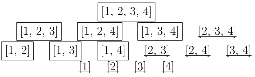
Example: Now, we give an example to illustrate how the TSF of a subspace is computed at
[1, 2, 3, 4]
[1, 2, 3] [1, 2, 4] [1, 3, 4] [2, 3, 4]
[1, 2] [1, 3] [1, 4] [2, 3] [2, 4] [3, 4] [1] [2] [3] [4]
Figure 5: Subspaces of a 4-dimensional full space
Dimension of subspaces TSF
4 28
3 13
2 12
1 19
(a)
Dimension of subspaces TSF
3 9
2 10
1 17.7
(b)
Dimension of subspaces TSF
3 2.7
2 2
(c)
Table 2: Computation of Dyna-CSF
each of the tables. According to the tables, the order of subspaces in the search process is 4 → 1 → 3 → 2, meaning that the 4 dimensional subspaces are searched first, followed by 1 dimensional and 3 dimensional subspaces. The 2 dimensional subspaces are searched at last. The probabilities of upward and downward pruning of this sample point in different dimensions, starting from 1 to d dimension with the format of{prup(m, sp),prdown(m, sp)},
are {0.25, 0},{0.5,0.5},{0.75,0.25}and {0, 0}.
Table 3 summarizes the subspaces searched for the three search methods, i.e. top-down, bottom-up and dynamic search.
4.5 Minimum Sampling Size for Training Dataset
Before moving on to the details of the HighDOD algorithm, it is worthwhile to discuss the minimum sample size used for the training dataset.
Recall the sampling method is utilized to obtain a training dataset that can be used to pre-compute the prior probabilities of upward and downward pruning, namely prup(m)
and prdown(m) (1 ≤m≤ d). As such, samples of different sizes will only affect the pruning
efficiency of the algorithm. They will not change the number of subspaces found.
With this in mind, we now wish to determine the minimum sample size to accurately predict prup(m) and prdown(m) with certain degree of confidence. We denote X as the
Searching methods Subspace searched
Top-down searching [1,2,3,4],[1,2,3],[1,2,4],[1,3,4], [2,3,4], [1,2],[1,3],[1,4],[1] Bottom-up searching [1], [2], [3], [4], [2,3], [2,4],[3,4], [2, 3,4]
[image:13.595.115.502.71.132.2]Dynamic searching [1,2,3,4], [1], [2], [3], [4], [2,3,4]
Table 3: Pruning results of three methods
where S is the size of the sample. Each data in the sample is a d-dimensional vector as xi = [xi,1, xi,2, . . . , xi,d]T where xi,j denote the value of jth dimension of ith data in the
sample. Applying dynamic subspace searching on sampling points, for each dimension m, we obtain
Ydown(m) = [prdown(m, sp1), prdown(m, sp2), . . . , prdown(m, spS)] (1≤m ≤d)
We use theS measurements,prdown(m, spi)(1 ≤i≤S) as the training data to estimate
the mean ofprdown(m). Here, we assume that the training data are independent and can be
approximated by Gaussian distribution. We estimate the sample size by constructing the confidence interval of the mean of prdown(m). Specifically, to obtain a (1−α)-confidence
interval, the minimum size of a random sample is given as follows [15]:
Smin(m) = [
tα/2∗σ
′ m
δ∗ ]
2
whereσ′
m denotes the estimated standard deviation ofprdown in themthdimension using the
training points that is defined as:
σm′ = v u u t
S
X
i=1
(prdown(m, spi)−prdown(m, sp))2/(S−1)
δ∗ denotes the half-width of the confidence interval.
Note that the value of σm′ varies for different m. Let σmax′ = max(σ′m)(1 ≤ m ≤ d), the minimum sample size Smin that satisfies respective minimum sample size requirement of
each dimension is computed as:
Smin = [
tα/2∗σ
′ max
δ∗ ]
2
Similarly reasoning applies to prup(m) since prup(m)= 1- prdown(m).
4.6 Applicability of Existing High-dimensional Outlier Detection
Technique
formulated as follows: Given a data point p, find all the subspaces in which p is an outlier based on the information of outliers in each subspace that is obtained by the ”subspace→ outliers” high-dimensional outlier detection technique. To solve this problem, a searching in all subspaces is needed in order to find the set of outlying subspaces of p: the outlying subspaces forpare those subspaces in whichpis in their respective set of outliers. Obviously, the computational and space costs are both proportional to the total number of subspaces which is in an exponential order ofd, where d is the number of dimension of the data point. This analysis provides an insight into the inherent difficulty of using the existing high-dimensional outlier detection techniques to solve the new ”outlier-subspaces” problem espe-cially in a high-dimensional space where such a space searching is rather expensive.
5. Algorithms
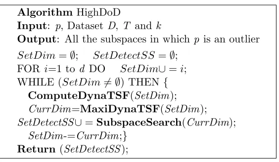
The algorithm of dynamic subspace search is presented in Figure 6. In this algorithm,
SetDim stores the number of dimension of the subspaces (from 1 to d). When SetDim is not empty, it indicates that there are still some subspaces to be searched. The new TSF of the remaining dimensions are computed and an additional pass of the subspace search is performed. The dimension of the subspace with the maximum TSF in the current step is stored in the variableCurrDim. The current dimension of subspaces is deleted fromSetDim
and the whole program terminates whenSetDim becomes empty. All the subspaces detected are saved in SetDetectSS. This is returned as the answer set to the user at the end of the algorithm. Note that the algorithm presented in Figure 6 can run on both the sample points and the query points. The only difference is in the function ComputeDynaTSF(). Here, the sample points use the pre-defined probabilities as the priors while the query points use the probabilities as the priors obtained in the sample-based learning process. The function of ComputeDynaTSF() dynamically computes the TSF values in the subspace searching process. The upper bound of the number of dimensions in SetDim is d, thus the time complexity of performing this function is O(d).
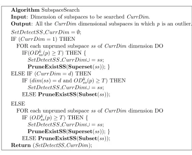
The function SubspaceSearch() (referring to Figure 7 for details) returns all the de-tected subspaces of the CurrDim dimension. It displays a generic skeleton of the function SubspaceSearch() for subspace searching using either the global-T pruning strategy or the local-T pruning strategy. Note that there are two differences between the exact implemen-tation of the function for the two pruning strategies: (1) T represents the global distance threshold in the global-T pruning strategy while represents the local distance threshold for each subspacesswithCurrDim dimension in the local-T pruning strategy; (2) In the local-T pruning strategy, the algorithm has to check the satisfiability of the pruning requirements within the functions P runeExistSS(superset(ss)) and P runeExistSS(subset(ss)) before the pruning is performed, while the global-T pruning strategy does not have to.
6. Experimental Results
AlgorithmHighDoD
Input: p, Dataset D,T and k
Output: All the subspaces in which p is an outlier
SetDim=∅; SetDetectSS=∅; FOR i=1 to d DO SetDim∪=i; WHILE (SetDim6=∅) THEN {
ComputeDynaTSF(SetDim);
CurrDim=MaxiDynaTSF(SetDim); SetDetectSS∪=SubspaceSearch(CurrDim);
SetDim-=CurrDim;}
[image:15.595.167.449.68.232.2]Return(SetDetectSS);
Figure 6: Algorithm of dynamic subspace search
UCI machine learning repository, which have been utilized in [4] for performance evaluation, are also used.
In the synthetic data generator, we can specify the number of instances (tuples) (N) and dimensions (d) of the dataset generated. We will further specify the number of the ranges (Nr) and the maximum (max) and minimum (min) values for each dimension of the dataset.
The interval for each of the ranges will be max−minNr . For each of the dimensions, NNr distinct instances are generated based on the Gaussian distribution in each of theNr ranges. In this
way, we will be able to obtain N distinct instances for each dimension. For each generated instance, a random number i (1≤i≤N) will be generated (without replacement) and this instance will be assigned to the ith tuple in the dataset. The dataset generated generally
displays dense and sparse regions in the data space, which serves as an ideal test-bed for our experiments. Specifically, we specify N from 100k to 1000k, d from 10 to 100, and for each dimension, we specify Nr = 10, min= 0, max= 100 in our experimental setting.
All the algorithms are implemented on a 1.8GHz Pentium PC with 256 MB of main memory running on Windows 2000. In all the experiments, we setk, the number of neighbors we are interested in, to 10.
6.1 Efficiency Study
AlgorithmSubspaceSearch
Input: Dimension of subspaces to be searchedCurrDim.
Output: All the CurrDim dimensional subspaces in which p is an outlier.
SetDetectSS CurrDim=∅; IF (CurrDim= 1) THEN
FOR each unpruned subspace ss of CurrDim dimension DO IF(ODssk(p)≥T) THEN {
SetDetectSS CurrDim∪=ss;
PruneExistSS(Superset(ss)); }
ELSE IF (CurrDim=d) THEN
IF (dim(ss) =dandODkss(p)≥T) THEN
SetDetectSS CurrDim∪=ss;
ELSEPruneExistSS(Subset(ss));
ELSE
FOR each unpruned subspace ss of CurrDim dimension DO IF (ODkss(p)≥T) THEN {
SetDetectSS CurrDim∪=ss;
PruneExistSS(Superset(ss)); }
ELSEPruneExistSS(Subset(ss));
[image:16.595.116.493.61.365.2]Return(SetDetectSS CurrDim);
Figure 7: The generic algorithm of searching subspaces of a given dimension
all subspaces of different dimensions and selects the best subspaces to begin the search. To evaluate the efficiency of the sample-based learning process in reducing the search space, we run the dynamic search algorithm with and without incorporating the sample-based learning process. Since there are two pruning strategies, i.e. the Global-T and the Local-T pruning strategy, thus we implement the above five searching methods with each of the two pruning strategies, which resulting in a total of 10 searching methods. Note that the execution times shown in this section are the average time spent in processing each point in the learning and query process.
In the first set of experiments, we investigate the effect of dimensions on the average execution time of the algorithm. Figure 8 shows the results as we vary the dimensions of the datasets. A quick review of the result reveals that the execution time of all the 10 methods increase at an exponential rate since the number of subspaces increases exponentially as the number of dimension goes up, regardless of which searching and pruning strategy is utilized. On a closer examination, we see that (1) The execution time of top-down and bottom-up search methods increase much faster than the dynamic search method; (2) When using the sample-based learning process, the dynamic search method performs better than without using the sample-based learning process; (3) The execution times of the methods using the Global-T pruning strategy increase much less slowly compared with the whose methods using the Local-T pruning strategy. This is because the Local-T pruning strategy is much conservative than the the Global-T pruning strategy and therefore less number of subspaces can be pruned in each step of the searching process.
10 20 30 40 50 60 70 80 90 100 0 100 200 300 400 500 600 700 800 900 1000
Number of dimensions (N=100k, Nq=200)
Average CPU execution time (Sec.)
[image:17.595.101.288.73.218.2]Top−down (Global−T) Bottom−up (Global−T) Random (Global−T) Dynamic (Global−T) Sample−based dynamic (Global−T) Top−down (Local−T) Bottom−up (Local−T) Random (Local−T) Dynamic (Locall−T) Sample−based dynamic (Local−T)
Figure 8: Execution time when vary-ing dimension of data
100 200 300 400 500 600 700 800 900 1000 0 200 400 600 800 1000 1200 1400 1600
Size of dataset (K) (d=50, nq=200)
Average CPU execution time (Sec.)
[image:17.595.321.509.73.218.2]Top−down (Global−T) Bottom−up (Global−T) Random (Global−T) Dynamic (Global−T) Sample−based dynamic (Global−T) Top−down (Local−T) Bottom−up (Local−T) Random (Local−T) Dynamic (Local−T) Sample−based dynamic (Locall−T)
Figure 9: Execution time when vary-ing size of dataset
50 100 150 200 250 300 350 400 450 500 40 50 60 70 80 90 100 110 120
Number of query points (N=100,000, d=50)
Average CPU execution time (Sec.)
Top−down Bottom−up Dynamic
Sample−based dynamic
Figure 10: Execution time when varying the number of query points
20 40 60 80 100 120 140 160 180 200 50 60 70 80 90 100 110 120
Number of sampling points (N=100,000, d=50, Nq=200)
Average CPU execution time (Sec.)
Dynamic
Sample−based dynamic
Figure 11: Execution time when varying the size of sample
size of datasets from 100K to 1,000K. Figure 9 shows that the average execution times using the 10 methods to process each query point are approximately linear with respect to the size of the dataset. Similar to results of the first experiment, the dynamic search method with sample-based learning process and Global-T pruning strategy gives the best performance.
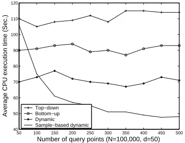
Next, we vary the number of query points Nq. Figure 10 shows the results of the
five searching method using the Local-T pruning strategy only . It is interesting to note that whenNq is large, dynamic search method with sample-based learning process gives the
best performance. However, when Nq is small, it is better to use dynamic search without
sample-based learning. The reason is because when the number of query points is small, the saving in computation by using the learning process is not sufficient to justify the cost of the learning process itself.
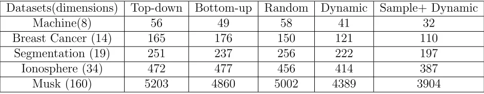
[image:17.595.324.510.274.425.2] [image:17.595.100.289.275.421.2]Datasets(dimensions) Top-down Bottom-up Random Dynamic Sample+ Dynamic
Machine(8) 56 49 58 41 32
Breast Cancer (14) 165 176 150 121 110
Segmentation (19) 251 237 256 222 197
Ionosphere (34) 472 477 456 414 387
[image:18.595.72.544.73.165.2]Musk (160) 5203 4860 5002 4389 3904
Table 4: Results of running five methods on real-life datasets (average CPU time in seconds for each query point)
Furthermore, a closer examination of the result reveals that using dynamic subspace search alone is faster than top-down bottom-up or random search methods by approximately 20% while incorporating sample-based learning process into dynamic subspace search contributes to reducing the execution time by about 30%.
6.2 Effect of Sampling Size on the Efficiency of HighDOD
We also investigate the effect of the number of sampling points, S, used in the learning process. A large S gives a more accurate estimation of the possibilities of upward and downward pruning in subspaces, which in turn, helps to speedup the search process. However, a largeS also implies an increase in the computation during the learning process, which may increase the average time spent in the whole outlier detection process. As we can see, the execution time is first decreased when the number of sampling point is small, this is because the prediction of possibility is not accurate enough, which cannot greatly speedup the later searching process. When the sample size increases, the prediction of the possibilities are sufficiently accurate, therefore any larger size of sample will no longer contribute to the speedup of the search process, but only increase the execution time as a whole. Furthermore, the sample size corresponding to the valley value of the CPU runtime in the figure is close toSmin, indicating thatSmin is an optimal or at least near-optimal sample size to choose in
practice. The horizontal dot-line in Figure 11 indicates the execution time when dynamic subspace search without sample-based learning is employed. We can see that a large size of sample will cause the average execution time exceed the horizontal line, thus a sample of reasonably small size (such like Smin) will ensure that the speedup of the searching process
will not be overshadowed by the associated cost of the learning process.
7. Conclusions
a dynamic subspace search method with a sample-based learning process. Experimental results indicate that our method is efficient and outperforms the straightforward top-down, bottom-up and random search methods.
References
[1] R. Agrawal, J. Gehrke, D. Gunopulos, and P. Raghavan. Automatic Subspace Clustering of High Dimensional Data Mining Application. Proc. ACM SIGMOD’99, Philadelphia, PA, USA, 1999.
[2] F. Angiulli and C. Pizzuti. Fast Outlier Detection in High Dimensional Spaces. Proc.
PKDD’02, Helsonki, 2001.
[3] C. C Aggarwal, C. Procopiuc, J. L. Wolf, P. S Yu and J. S. Park. Fast Algorithms for Projected Clustering. Proc.ACM SIGMOD’99, Philadelphia, Pennsylvania, USA, 1999.
[4] C. C Aggarwal and P.S. Yu. Outlier Detection in High Dimensional Data. Proc. ACM SIGMOD’00, Santa Barbara, California, 2001.
[5] V. Barnett and T. Lewis. Outliers in Statistical Data. John Wiley, 3rd edition, 1994.
[6] S. Berchtold, D. A. Keim and H. Kriegel. The X-tree: An Index Structure for High-Dimensional Data. Proc. VLDB’96, Mumbai, India, 1996.
[7] M. Breuning, H-P, Kriegel, R. Ng, and J. Sander. LOF: Identifying Density-Based Local Outliers. Proc. ACM SIGMOD’00, Dallas, Texas, 2000.
[8] M. Ester, H-P Kriegel, J. Sander, and X.Xu. A Density-based Algorithm for Discovering Clusters in Large Spatial Databases with Noise. Proc. SIGKDD’96, Portland, Oregon, USA, 1996.
[9] J. Han and M. Kamber. Data Mining: Concepts and Techniques. Morgan Kaufman Publishers, 2000.
[10] D. Hawkins. Identification of Outliers. Chapman and Hall, London, 1980.
[11] A. Hinneburg, and D.A. Keim. An Efficient Approach to Cluster in Large Multimedia Databases with Noise. Proc. SIGKDD’98, 1998.
[12] W. Jin, A. K. H. Tung, J. Han. Finding Top n Local Outliers in Large Database. Proc.
SIGKDD’01, San Francisco, CA, August, 2001.
[13] E. M. Knorr and R. T. Ng. Algorithms for Mining Distance-based Outliers in Large Dataset. Proc. VLDB’98, pages 392-403, New York, NY, August 1998.
[14] E. M. Knorr and R. T. Ng. Finding Intentional Knowledge of Distance-based Outliers. Proc. VLDB’99, pages 211-222, Edinburgh, Scotland, 1999.
[16] R.Ng and J.Han. Efficient and Effective Clustering Methods for Spatial Data Mining. Proc. VLDB’94, pages 144-155, 1994.
[17] F. Preparata and M. Shamos. Computational Geometry: an Introduction. Springer-Verlag, 1988.
[18] S. Ramaswamy, R. Rastogi, and S. Kyuseok. Efficient Algorithms for Mining Outliers from Large Data Sets. Proc. ACM SIGMOD’00, Dallas, Texas, 2000.
[19] I. Ruts and P. Rousseeuw. Computing Depth Contours of Bivariate Point Clouds. Com-putational Statistics and Data Analysis. 23: 153-168, 1996.
[20] G. Sheikholeslami, S. Chatterjee, and A. Zhang. WaveCluster: A Wavelet based Clus-tering Approach for Spatial Data in Very Large Database. VLDB Journal, vol.8 (3-4), 289-304, 1999.