Volatility modeling and prediction: the role of price
impact
University of Nottingham Ningbo China, 199 Taikang East Road, Ningbo,
315100, Zhejiang, China.
First published 2019
This work is made available under the terms of the Creative Commons
Attribution 4.0 International License:
http://creativecommons.org/licenses/by/4.0
The work is licenced to the University of Nottingham Ningbo China
under the Global University Publication Licence:
https://www.nottingham.edu.cn/en/library/documents/research-support/global-university-publications-licence.pdf
Volatility modeling and prediction: The role of price impact∗
Ying Jiang† Yi Cao‡ Xiaoquan Liu§ Jia Zhai¶
April, 2019
Abstract
In this paper, we are interested in exploring the role of price impact, derived from the order book, in
modeling and predicting stock volatility. This is motivated by the market microstructure literature that
examines the mechanics of price formation and its relevance to market quality. Using a comprehensive
dataset of intraday bids, asks, and three levels of market depths for 148 stocks in the Shanghai Stock
Exchange from 2005 to 2016, we find substantial intraday impact from incoming bid and ask limit
and market orders on stock prices. More importantly, the permanent price impact at the daily level
is a significant determinant of stock volatility dynamics as suggested by the panel VAR estimation.
Furthermore, when we augment traditional volatility models with the time series of daily price impact,
the augmented models produce significantly more accurate volatility predictions at the one-day ahead
forecasting horizon. These volatility predictions also offer economic gains to a mean-variance utility
investor in a portfolio setting.
JEL code: C53, G14
Keywords: Market Microstructure; Chinese Stock Market; Panel Vector Autoregression; Volatility Mod-eling.
∗
Financial support from the Chinese Ministry of Education Grant No. 17YJA790037 is gratefully acknowledged. We thank an anonymous referee whose thorough comments have substantially improved the paper. Thanks are also due to audiences and discussants at China Finance Review International Conference in Shanghai in June 2018 and the Asian Financial Association conference in Tokyo in July 2018 for helpful comments.
†
Nottingham University Business School China, University of Nottingham Ningbo, Ningbo 315100, P. R. China. Email: ying.jiang@nottingham.edu.cn.
‡
Management Science and Business Economics Group, University of Edinburgh Business School, 29 Buccleuch Place, Edinburgh EH8 9JS, UK. Email: jason.caoyi@gmail.com.
§
Corresponding author. Nottingham University Business School China, University of Nottingham Ningbo, Ningbo 315100, P. R. China. Email: xiaoquan.liu@nottingham.edu.cn.
¶
1
Introduction
Intraday price formation and variation is a central topic in the market microstructure literature dating back a few decades. French and Roll (1986) is an early effort which shows that stock volatility is signifi-cantly higher during trading hours than during non-trading hours and attributes this to microstructure phenomenon. Both theoretical and empirical studies focus on examining the sources of these intraday price variations. Many argue that order book events are a conduit for volatility information and, intu-itively, stock return volatility is partially determined by microstructure noise generated in the trading process. Madhavan et al. (1997) develop a theoretical model and decompose determinants of stock volatil-ity into public news and microstructure-induced noise, i.e., effective bid-ask spread; and Ahn et al. (2001) establish a bilateral relation between transitory volatility and order flow. These results are in line with those from Foucault (1999), Foucault et al. (2007), and Handa and Schwartz (1996).
Motivated by this strand of the literature, we explore in this paper whether the information content of order book events such as the arrival of limit and market orders and trades is an important driver of stock volatility in-sample. If the answer is affirmative, we are also interested in knowing whether the time series of price impact is able to improve the precision of out-of-sample volatility predictions, both in statistical and economic terms. Hence our paper crosses over between two important fields in finance, i.e. market microstructure and volatility prediction, and extends the existing literature in which microstructure information is adopted for the purpose of volatility modeling and forecasting such as bid-ask spread (Bollerslev and Melvin, 1994); information flow (Gallo and Pacini, 2000); and trading volume (Wagner and Marsh, 2005) in a GARCH-X type model.
Our empirical analysis is conducted on the Chinese stock market, a major order-driven emerging market that enjoys exponential growth since its inception. Established in 1990, the Shanghai Stock Ex-change (SSE) started with only eight listed stocks but over less than three decades it now trades more than 1400 stocks with a total market capitalization of RMB 30 trillion as of July 2018.1 During this period, the market has experienced a number of major policy shocks such as the ownership structure
1
reform in 2005 and more recently the ill-fated circuit breaker regulation in 2016. The less-than-stable institutional environment may induce a different information reflection process in equity prices. Equally importantly, the market is characterized by a disproportion of individual investors compared with devel-oped equity markets hence the price dynamics from order book events could be different as suggested by the asymmetric information theory (Milgrom and Stokey, 1982; Kyle, 1985). Our sample consists of 148 firms traded on the SSE, all of which are component stocks of the Chinese CSI 300 index, and covers a variety of sectors. The data are intraday bid and ask quotes over three depth levels over a long sample period from January 2005 to August 2016.2
We contribute to the literature by offering a comprehensive study that explores the price impact of order book events in this young, dynamic yet important emerging market, and reveals how the price impact of incoming orders affects volatility and improves its prediction accuracy.3 Methodologically, we first follow Hautsch and Huang (2012) and estimate the price impact of incoming limit and market orders by a vector autoregression (VAR) framework. The econometric framework is able to consider the short-and long-run impact of buy short-and sell orders via impulse response functions. We then investigate whether the price impact significantly affects stock volatility via a panel VAR model that allows us to evaluate the price impact on the volatility of all sample stocks simultaneously. Finally, we include the price impact as additional variable in two commonly used volatility models, the standard GARCH model of Bollerslev (1986) and the heterogeneous auroregressive (HAR) realized volatility model of Corsi (2009), and compare the forecasting accuracy of the augmented models with the original models in statistical and economic terms.
We reveal a host of interesting findings. First, we document substantial price impact of incoming limit and market orders similar in magnitude to that of developed markets (Hautsch and Huang, 2012), and a significant relation between price impact and volatility in the Chinese equity market. Both ask and bid prices tend to shift significantly after the arrival of a buy or sell limit or market order. The impact is, 2 Our sample compares favourably to 50 US stocks for a sample period of 21 days in Cont et al. (2014); 30 stocks in the
Euronext Amsterdam exchange with a two-month sample periods in Hautsch and Huang (2012); and 100 stocks in Nasdaq over two years in Engle and Patton (2004).
3The only related study is Jain and Jiang (2014), which shows that the limit order book slope consistently and significantly
however, asymmetric: we show that the magnitude of price impact induced by a market order is generally larger than that by a limit order. We also notice that the arrival of a sell market order gives rise to a larger impact on ask or bid prices than a buy market order. The permanent price impact induced by incoming limit and market orders is highly significant, indicating that incoming orders contain substantial information and contributes to the price discovery process. This is consistent with the existing literature that order book events play an important role in the price formation process in many developed markets. Second, adopting a panel VAR model which allows us to gauge the effect of permanent price impact series on all sample stocks, we show that changes in aggregate daily price impact cause significant changes in stock volatility. This is the first piece of evidence on the link between stock volatility and the price impact of incoming limit or market orders and in line with the theoretical framework in Madhavan et al. (1997) that microstructure noise is an integral part of the information source for volatility.
Third, by adding daily permanent price impact to GARCH and HAR models, the out-of-sample accuracy of volatility forecasts is significantly improved. We adopt the popular Diebold and Mariano (1995) pairwise comparison and show that the augmented GARCH-X and HAR-X models with the time series of price impact consistently produce statistically smaller forecasting errors across three different loss functions. Furthermore, for a mean-variance utility investor who allocates her wealth between a stock and the riskfree asset, the volatility predictions from augmented models lead to significantly higher annualized portfolio returns, Sharpe ratio, and certainty equivalent returns in a portfolio setting across a range of risk aversion levels. These novel findings support our conjecture that price impact of incoming order book events contains valuable information for volatility and adding the information improves volatility forecasting precision in statistical and economic terms.
2
Literature review
In an order-driven market there is no designated market maker for liquidity provision. Instead traders choose to submit limit and/or market orders which will automatically be matched by an electronic trading system and thus change the pending volume and the best bid or ask quotes. Glosten (1994) derives the equilibrium price determined by bid and ask quotes in an open order book for an order-driven market; while Foucault (1999), Foucault et al. (2005), Goettler et al. (2005), Goettler et al. (2009), Rosu (2009) capture the dynamics of a limit-order market via game theoretic models. To date, limit order trading has been examined worldwide in the NASDAQ (Cont et al., 2014; Eisler et al., 2012), the Deutsche Boerse (Riordan and Storkenmaier, 2012), the Oslo Stock Exchange (Naes and Skjeltorp, 2006), the Paris Bourse (Biais et al., 1995, 1999), the Euronext Amsterdam (Hautsch and Huang, 2012), the Tokyo Stock Exchange (Hamao and Hasbrouck, 1995; Lehmann and Modest, 1994), the Australian Stock Exchange (Cao et al., 2009), and the Heng Seng Stock Exchange (Ahn et al., 2001).
characteristics and provides a comprehensive description of the order book.
Meanwhile, the importance of volatility, which is central to portfolio allocation, derivative valuation, and risk management, is well documented. The literature on volatility modeling has made significant advancement since the seminal work of Engle (1982) (see Andersen et al., 2003; Engle et al., 2013; Hansen and Lunde, 2011). One strand in this literature extends volatility modeling by incorporating market microstructure variables in low-order ARCH family of volatility models. Bollerslev and Melvin (1994) document empirical evidence that the size of bid-ask spread in the foreign exchange market is related to the exchange rate volatility in a GARCH framework. This is consistent with theories of asymmetric information in bid-ask spreads. Adding a measure of overnight information flow between market close and open, Gallo and Pacini (2000) reveal a significant relation between this measure and stock volatility in GARCH and EGARCH settings. Furthermore, trading volume is another popular microstructure measure extensively explored in the volatility literature and shown to relate to asset volatility (see Fleming et al., 2008; Lamoureux and Lastrapes, 1990; Wagner and Marsh, 2005). Our paper is motivated by and contributes to both strands of the literature.
3
Econometric framework
We first follow Hautsch and Huang (2012) in modeling and quantifying price impact via a restricted VAR model.4 The vector of variables includes the logarithmic values of best bid/ask limit and market quotes, the best three volumes on both sides of bid and ask for limit and market orders, and trades. The short- and long-run price impacts are estimated via the impulse response function of the VAR and the long-run impact is considered the permanent price impact and included in the volatility forecasting exercise. The details of the VAR model are summarized in Appendix A. In this section, we focus on the panel VAR (PVAR) model to examine the relevance of price impact to stock volatility in-sample, and how the information can be utilized in out-of-sample forecasting exercises.
3.1 The PVAR model
Given the theoretical and empirical evidence on the relationship between market microstructure vari-ables and asset volatility, we hypothesize that the price impact of incoming orders exerts significant impact on stock volatility. We use permanent price impact of incoming limit and market orders since it represents equilibrium price changes induced by order book events. We adopt a VAR framework in which all variables are treated as endogenous and interdependent both in a dynamic and a static sense. The impulse response function of the VAR system is able to reflect the change in one variable driven by the change in others.
We construct the VAR system that includes daily stock volatility estimated by the GARCH or the HAR model, and daily permanent price impact induced by arriving bid and ask limit and market orders. We use daily data as it is the most commonly used frequency in the volatility forecasting literature. The price impact series for each stock are estimated at the intraday frequency through the impulse response function in Eq. (A8) based on the estimation of the VAR model in Eq. (A2), and aggregated to daily level by adding intraday observations.
Following Abrigo and Love (2016a), we define the k-variate homogeneous PVAR model of order p
with panel-specific fixed effects as follows:
Yid =Yid−1A1+Yid−2A2+...+Yid−p+1Ap−1+Yid−pAp+ui+eid, (1)
where i = 1,2, . . . , N, and N is the number of panels, i.e. the number of stocks in our sample; d =
1,2, . . . , Di, and Di is the number of days in the sample for each stock i. For each panel, Yid is a 1×k
vector of dependent variables; ui and eid are 1×k vectors of dependent variable-specific panel
fixed-effects and idiosyncratic errors, respectively; the k×k matrices A1, ..., A2, Ap−1, Ap are parameters to
be estimated. Consistent parameters are obtained via an equation-by-equation generalized method of moments (GMM) procedure (Abrigo and Love, 2016a).
To investigate the relationship between price impact and volatility, the impulse response function specified in the PVAR model is of great interest. Re-writing the model as an infinite vector moving average (VMA), the simple impulse response function Φl can be expressed as follows:
Φl=
Ik, l= 0
Pl
j=1Φd−jAj, l > 0
(2)
where Φl are the VMA parameters. In our study, we adopt the bootstrap re-sampling method following
Kapetanios (2008) with 100 Monte Carlo draws to estimate the confidence interval of the impulse response function. The system of PVAR is constructed as follows:
Yid= [Volid,LBid2Pid,LAsk2Pid,MBid2Pid,MAsk2Pid]T , (3)
where for stock i on day d, Volid denotes stock volatility, which is proxied by the GARCH volatility in
Eq. (5) or the realized volatility in Eq. (6) specified below. Furthermore, LBid2Pid and LAsk2Pid are
the permanent price impact incurred by bid limit orders and ask limit orders, respectively; and MBid2Pid
respectively, for stock ion day d. They are obtained by aggregating intraday price impact to the daily level following Eq. (A8).5
3.2 Volatility modeling and forecasting
The GARCH model
The generalized autoregressive conditional heteroskedasticity (GARCH) model of Bollerslev (1986) takes account of the time-varying volatility clustering of most financial time series and has been widely applied in many studies (see Andersen and Bollerslev, 1998b; Chortareas et al., 2011; Glosten et al., 1993; Jiang et al., 2017; Martens, 2001). We use the most parsimonious GARCH (1,1) in our study:
ηd = µ+d, d|Ωd−1∼tv(0, σd2), (4)
σd2=κ+βσ2d−1+α2d−1, (5)
whereηdrepresents daily return series as the difference between the logarithmic prices on daydand day
d−1,µ is the mean,d is the innovation conditional on the information set and follows at-distribution
denoted by tv with zero mean, variance σ2d, and v degrees of freedom. In addition, β is the GARCH
component coefficient and α is the ARCH component coefficient. The GARCH model requires that
α+β <1 for the volatility process to be stationary. Note that the volatility σd estimated in Eq. (5) is
used in the PVAR of Eq. (3).
The HAR model
Proposed by Corsi (2009), the HAR model is a simple AR-type model in realized volatility that considers different volatility components realized over different time horizons. We choose this model for its ability of capturing the main empirical characteristics of financial returns such as long memory, fat tails and multi-scaling which cannot be handled by traditional short-memory models such as the GARCH. The
5
HAR model also overcomes undesirable features of fractional integration models such as artificially mixing long- and short-term characteristics, difficulty in estimation, and inability in handling the multi-scaling feature (Comte and Renault, 1998). Most importantly, it exhibits remarkable forecasting performance (Corsi, 2009) and hence has been widely adopted in the literature (see Chiriac and Voev, 2011; Dimpfl and Jank, 2016; Fernandes et al., 2014; Hillebrand and Medeiros, 2010, for example). The model includes additive cascade of volatility components defined over different time horizons as follows:
RVd(d)=c+β(d)RVd(−d)1+β(w)RVd(−w1)+β(m)RVd(−m1)+(dd), (6)
whereRVd(d),RVd(w), andRVd(m)represent daily, weekly and monthly volatility components, respectively, on day d. The daily realized volatility RVd(d) is calculated by aggregating intraday squared returns as shown in Eq. (9) below. The weekly and monthly realized volatilities are simple averages of the daily realized volatility:
RVd(w)= 1
5
RVd(d)+RVd(−d)1+· · ·+RVd(−d)4
, (7)
RVd(m)= 1
22
RVd(d)+RVd(−d)1+· · ·+RVd(−d)21
. (8)
Irrespective of their actual frequency, volatility quantities are annualized to facilitate comparison between different frequencies. Note that the realized volatility RVd(d) estimated in Eq. (6) is used in the PVAR of Eq. (3).
Proxy for latent volatility dynamics
The true volatility is an unobservable latent variable. In the literature, the most popular proxy is the realized volatility (RV) proposed by Andersen and Bollerslev (1998a). This is obtained by aggregating intraday squared returns. We follow this approach and construct a realized volatility series using 4-6 second logarithmic return series as follows:
ˆ
σrv,d2 =
T
X
t=1
where ˆσrv,d is the realized volatility for daydandr2d,tis the squared intraday logarithmic return on dayd
for time indext(t= 1,2, ..., T). We use ˆσrv,das the proxy for the true volatility to evaluate the accuracy
of out-of-sample forecasting performance in Eqs. (13)-(15).
Forecasting models
To incorporate information content of price impact into volatility forecasting, we include the time series of permanent price impact of incoming buy and sell limit and market orders into the baseline GARCH and HAR models in Eq. (5) and Eq. (6), respectively, and formulate the GARCH-X and HAR-X models to produce out-of-sample volatility forecasts. The factor HAR-X in the GARCH-HAR-X and HAR-HAR-X models are either the permanent price impact of buy and sell limit orders or the permanent price impact of buy and sell market orders. The GARCH (1,1)-X model is defined as follows:
ηd=µ+d, d|Ωd−1 ∼tv(0, σ2d), (10)
σd2 =κ+βσ2d−1+α2d−1+γ1LBid2Pd−1+γ2LAsk2Pd−1, (11a)
σd2 =κ+βσ2d−1+α2d−1+γ1MBid2Pd−1+γ2MAsk2Pd−1. (11b)
We include the price impact of limit and market orders separately into the model to distinguish their information content for volatility modeling for each stock resulting in 148×2 estimations. Similarly, we do the same to form a HAR-X model as follows:
RVd(d)=c+β(d)RVd(−d)1+β(w)RVd(−w1)+β(m)RVd(−m1)+γ1LBid2Pd−1+γ2LAsk2Pd−1+(dd), (12a)
RVd(d)=c+β(d)RVd(−d)1+β(w)RVd(−w1)+β(m)RVd(−m1)+γ1MBid2Pd−1+γ2MAsk2Pd−1+(dd). (12b)
Forecast evaluation
which is a more relevant task for investors and traders. Hence we compare the out-of-sample performance between benchmark GARCH and HAR models and augmented GARCH-X and HAR-X models. For each stock, we select the first 80% of data for the in-sample estimation and use the remaining for out-of-sample prediction. We use a rolling window scheme and compute one-day ahead forecast. We evaluate the forecasting accuracy using three popular loss functions: the root mean squared error (RMSE), the mean absolute percentage error (MAPE), and the mean absolute error (MAE) as follows:
RMSE =
"
1
M
M
X
d=1
ˆ
vard+1−σˆ2rv,d+1
2 #12
, (13)
MAPE = 100
M
M
X
d=1
ˆ
vard+1−σˆ2rv,d+1
ˆ
σ2rv,d+1
, (14)
MAE = 1
M
M
X
d=1
varˆ d+1−ˆσrv,d2 +1
, (15)
where M is the number of days in out-of-sample period, ˆvard+1 is the one-day ahead forecasted variance
obtained either from Eqs. 11(a,b) or Eqs. 12(a,b), and ˆσrv,d2 +1 is the proxy for true variance in Eq. (9). The model with smaller forecasting error is not necessarily superior to competing models as the dif-ference between two forecasts can be insignificant statistically. To take such considerations into account, Diebold and Mariano (1995) (DM henceafter) propose a pairwise comparison test between two forecasting models. The DM statistic follows an asymptotic standard normal distribution under the null hypoth-esis. We implement the test to provide statistical evidence of whether an augmented volatility model outperforms the benchmark model in providing statistically more accurate forecasts. The test statistics is defined as follows:
DW = p1
MΩˆ
M
X
d=1
∆Lossd+1, (16)
where ∆Lossd+1 is the difference of forecasting errors between the benchmark and competing models,
and ˆΩ is the consistent estimate of the asymptotic variance M−0.5PM
d=1∆Lossd+1. The null hypothesis
is H0 :E[∆Lossd+1] = 0. A positive (negative) and significant t-statistic suggests that the competing
volatility forecasts.
Portfolio exercise
A strong statistical performance does not indicate economic gains to investors. Therefore we analyze the economic value of volatility forecasts assuming a mean-variance utility investor who allocates her wealth between one of the Chinese stocks in our sample and a risk-free asset. We follow Rapach et al. (2010) and Wang et al. (2016) to construct the utility function as follows:
Ud(rd) =Ed(wdrd+rd,f)−
1
2γσd(wdrd+rd,f), (17)
where on day d, wd is the weight of the stock in the portfolio, rd is the stock return in excess of the
risk-free rate, rd,f, andγ denotes the level of risk aversion. We maximize the utility functionUd(rd) with
respect to the weightwd and obtain the ex ante optimal weight on dayd+ 1:
ˆ
wd=
1
γ
ˆ
rd+1
ˆ
σ2
d+1
!
, (18)
where ˆrd+1 and ˆσd2+1 are the forecasted mean and volatility, respectively, of excess returns to the stock.
The risk-free rate is the short-term government lending rate.
Following Rapach et al. (2010) and Wang et al. (2016), we take the historical average as the mean forecasts for returns, ˆrd+1 = Pdj=1rj. Hence, for each level of risk aversion γ, the optimal weight
ˆ
wd= 1γ
ˆ
rd+1
ˆ
σ2
d+1
of the portfolio is only determined by the volatility forecasts as different strategies share the same mean forecasts of returns. We use the Sharpe ratio (SR):
SR = µ¯p ¯
σp
(19)
and the certainty equivalent return (CER):
CER = ˆµp−
γ
2σˆ
2
to evaluate the performance of the portfolio, where ¯µp and ˆµp are the mean portfolio excess returns atd
and d+ 1, respectively, and ¯σp and ˆσp2 are the standard deviation and variance of portfolio excess returns
atdandd+ 1, respectively. For robustness, we adopt γ=3, 6, and 9 to capture different levels of investor risk aversion.
4
Data and empirical results
Data
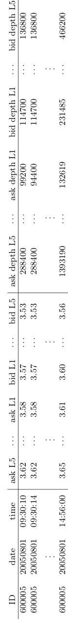
Our intraday data are obtained from the China Security Market Trade & Quote (Level 1) ofthe China
Stock Market & Accounting Research (CSMAR) database. We use stocks listed in the Shanghai Stock
Exchange which are component stocks of the Chinese CSI 300 index, also the largest and most liquid stocks across different sectors. We exclude the financial and banking sector and companies with less than three years of data. Our final sample includes 148 stocks with starting date ranging from August 2005 to May 2012 and the ending date is 31 August 2016 for most stocks. Table 1 summarizes descriptive statistics of 60 randomly selected stocks from our sample. The selected stocks cover 12 industries with a variety of sizes, turnovers, and growth prospects. The number of observations range from 1,890,581 to 7,095,527 due to different starting dates. In Table 2 we provide a cross-sectional snapshot of all sample firms by year. With such a comprehensive sample, our empirical findings are free from biases due to stock characteristics or sample period.
Table A2 tabulates the descriptive statistics of the daily permanent price impact of bid limit orders (LBid2P), bid market orders (MBid2P), ask limit orders (LAsk2P) and ask market orders (MAsk2P), respectively, for the first 30 selected stocks (code from 600009 to 600690) that are also shown in Table 1. These permanent price impacts are the long-term impulse response to incoming limit and market orders obtained via the VAR model. The average value for the price impact tends to be small with the order of magnitude at 10−3. Not surprisingly, the price impact from buy limit and market orders are positive, whereas that from sell limit and market orders are negative. The average of price impact shows that in most cases, the market orders generate greater price impact than limit orders.
Figure 1 illustrates typical price impact in the Chinese equity market. In this figure, we plot the instantaneous price impact for the Shanghai Electric Power company (Stock ID 600021) on a randomly selected trading day. The price impact is measured as the change in bid/ask price in basis point induced by a change in buy/sell limit or market orders equal to half the magnitude of level one depth against event time. We also show the 95% confidence interval of the price impact. We notice some interesting patterns. First, it is very clear that there exists substantial impact from the incoming limit or market orders to prices, both in the short- and long-run. This is consistent with the findings documented in Hautsch and Huang (2012) and suggests that in China, a young and emerging order-driven market, the price impact of order book events is as great as, if not more than, that in well developed equity markets. Second, the market order depicted in (c) and (d) of Figure 1 gives rise to greater permanent price impact compared with the limit order shown in (a) and (b). In terms of basis point, the price impact of the limit order is between -1 and 2.5 whereas for market orders it is between -8 and 4. This result is in line with the theoretical prediction in Rosu (2016) that informed traders choose to submit market order when the mispricing between the privately held fundamental asset value and the publicly expected fundamental value is substantial, which leads to greater price impact for market orders.
be submitted by informed or uninformed traders, it is ambiguous whether differences on the price impact between buy or sell limit orders exist.
Finally, for limit orders in (a) and (b) the price impact on the bid price converges to the permanent impact quicker than ask price; however for market orders in (c) and (d) the price impact on the ask price converges to the permanent impact sooner. This reflects different speed of price discovery process given different orders, i.e. buy or sell limit or market orders carry different information.
Although Figure 1 shows the price impact for one stock on a particular day, the patterns are repre-sentative of the price impact of order book events for the whole market. Once we establish the existence of substantial price impact in the Chinese equity market, we are interested in exploring how and to what extent the information content can be utilized in gauging the quality of the stock market, i.e. the volatility. We focus on the volatility as Ahn et al. (2001) and Madhavan et al. (1997) show in their theoretical framework as well as empirical evidence a link between intraday microstructure variables such as the bid-ask spread and order flow and intraday transitory volatility. We go one step further to explore whether this relation exists at the daily level between price impact and stock volatility.
hypothesis that the price impact is part of the information source that drives stock volatility.
Table 3 summarizes the in-sample parameter estimates for the GARCH-X and HAR-X models for selected stocks. For the GARCH-X model, we note that estimates for GARCH parameters α and β are both highly significant, and they add up to less than one indicating a stationary GARCH process. The coefficients γ1 and γ2, which are of great interest, capture the loading of permanent price impact in the
volatility model and they are highly significant at the 1% level for the majority of stocks, suggesting substantial impact of these variables on the in-sample volatility estimation. Meanwhile, for the HAR-X model, we find that theβ coefficient for the weekly realized volatility is highly significant at the 1% level consistently; whereas it is hardly significant for the daily and monthly realized volatilities. The in-sample estimation summarized in this table suggests that the price impact, when aggregated to the daily level, makes a significant contribution to volatility estimation.
the HAR model with an averaget-statistic of 10.17 using the MAE, and the minimum t-statistic is 8.01. These results support our conjecture that the information content of the price impact inferred from order book events, when aggregated to the daily level, is highly relevant and able to substantially improve the out-of-sample volatility prediction accuracy.
Statistical improvement does not indicate economic gains to investors when volatility predictions are used in trading strategies. Hence we conduct a simple portfolio exercise to gauge the economic value of volatility forecasts. As we assume that expected returns to individual assets are the same as their historical average, overall portfolio returns as well as weight for the stock hinge upon the accuracy of stock volatility forecasts and investor risk aversion. In Table 5 we summarize the cross-sectional average of annualized portfolio returns, the Sharpe ratio and the certainty equivalent return with three different risk aversion levels for benchmark GARCH and HAR models and augmented GARCH-X and HAR-X models for our sample stocks. The first thing we notice is that the cross-sectional average of portfolio return, the Sharpe ratio and the certainty equivalent return all increase significantly when we move from benchmark models to augmented models. This is shown by the high t-statistic in parentheses. For example, when the level of risk aversion is low atγ = 3 the market order price impact-augmented GARCH model offers an average annualized return of 6.12%, significantly higher than 5.32% by the benchmark GARCH model (t-statistic = 27.50). The Sharpe ratio increases from 0.28 to 0.33 (t-statistic = 25.58), whereas the certainty equivalent return goes up from 2.51% to 3.12% (t-statistic = 27.85). As the risk aversion level increases from 3 to 9, the returns and adjusted returns gradually drop but the pattern that the augmented models offer significantly improved portfolio returns, Sharpe ratio and certainty equivalent returns remains unchanged. This attests to the enhanced economic value of volatility forecasts when they contain information implied in the price impact.
5
Conclusion
the price formation in both quote- and order-driven markets. Furthermore, as volatility is shown to be partly driven by market microstructure related information, we are interested in knowing whether the information content of price impact extracted from order book events is relevant to volatility estimation and forecasting. We take these questions to the data and utilize quotes and three levels of market depths for 148 stocks traded on the Shanghai Stock Exchange, which are also component stocks for the Chinese CSI 300 index, between August 2005 to August 2016. Based on econometrics framework including the VAR and panel VAR models, we reveal a number of interesting findings. We show that there is substantial impact of incoming order book events on bid and ask prices in China, which is consistent with evidence in the existing literature on other equity markets. We further find that the time series of price impact are significant factors when added to traditional GARCH and HAR volatility models. More interestingly, the information content of the time series of price impact is able to significantly improve volatility prediction accuracy for individual stocks and offer economic gains to a mean-variance utility investor. Our comprehensive examination of the order book events is thus relevant to traders, fund managers and regulators alike.
Appendix A. The VAR model for price impact
To capture the dynamics of bid/ask quotes and depths and estimate the price impact induced by incoming limit and market orders, we use a restricted co-integrated VAR model, an appropriate model as ask and bid quotes are naturally integrated and tend to move in locksteps. The VAR has been used for measuring the price impact in Hasbrouck (1991), Easley et al. (1996), Engle and Patton (2004), and Hautsch and Huang (2012), among others. Following the specification in Hautsch and Huang (2012), we represent the limit order book system as a K= (4 + 2×k)-dimensional vector as follows:
yt= [pat, pbt, v
a,1
t , ..., v
a,k t , v
b,1
t , ..., v
b,k
where t denotes the time index for all order book activities, pat and pbt represent the logarithmic values of best ask and bid quotes instantaneously after the t-th order activity, and vta,k and vtb,k denote the logarithmic volumes at thek-th best ask and bid quotes, respectively. Hautsch and Huang (2012) suggest that aggressive limit orders placed close to the best ask and bid have the highest price impact while induced price effect massively declines down the depth level. We follow their method and focus on the best three quoted prices, denoted k = 1,2,3, in the empirical analysis. Buyt and Sellt are two dummy
variables indicating the occurrence of buy and sell trades, respectively. Using logarithmic values not only helps reduce the impact of very large observations but also implies that changes in market depth can be interpreted as relative changes with respect to the current depth level.
Hence we model the logarithmic bid and ask quotes, the corresponding volumes, and the trade dummy variables as a VAR(p) with the following vector error correction (VEC) form:
∆yt=µ+αβTyt−1+
p−1
X
i=1
Γi∆yt−i+ut, (A2)
where ut is the white noise with covariance matrix Σu, µ is a constant, Γi, i = 1, ..., p−1 is a K×K
parameter matrix, andαand βareK×r coefficient matrices withr < K.6 We estimate this VEC model using the Full Information Maximum Likelihood (FIML) estimator of Johansen and Juselius (1990) and Johansen (1991). To analyze the impulse response, we follow Lutkepohl and Reimers (1992) and transform the parameters of this VEC model to a reduced VAR representation as follows:
yt=µ+
p
X
i=1
Aiyt−i+ut,
where Ai = Γi−Γi−1, 1< i < p, A1 =IK+αβT + Γ1 and Ap =−Γp−1, while IK is a K×K identity
matrix.
The mechanics of price impact of incoming orders is as following: A limit order placed at the price equal to or lower (higher) than the best bid (ask) price will change the existing accumulated volume in 6 When estimating the cointegrating matricesαandβin Eq. (A2), we impose the restrictions on the first two columns
ofβ as follows: β1 = [0, ...,1,0]0 andβ2= [0, ...,0,1]0 for the trading indicator BUYt and SELLt, which are assumed to be
the order book. A limit order placed inside the spread, i.e. higher (lower) than the best bid (ask), will change the best bid (ask) as well. A market order will change the volume on the other side of the order book since it incurs immediate execution. If the size of a market order is larger than the volume at the first level on the other side, it will move the second best price on the other side aftereating up the volume at the first level.
We define shocks induced by incoming limit and market orders to the system of quotes, depths and trading indicators in terms of an impulse vector δ= [δp0, δv0, δ0d], withδp denoting a 2×1 vector consisting
of shocks to the quotes, δv being a 2k×1 vector associated with shocks to depth and δd being a 2×1
vector representing shocks to the trading indicator dummy. Imagine the following scenario: if a buy limit order is placed at the best bid price with half the size of vtb,1, where vtb,1 is the volume at the best bid price of order book at time t, the best bid and ask prices of the new order book remain the same thus
pat+1
pa
t = 1 and
pbt+1
pb t
= 1. The depth at the best bid level is aggregated to vb,t+11 = 1.5×vtb,1 but the depth at other levels remains the same. The shock vector δt, with elements of changes of quotes, depths and
trading indicators from time t tot+ 1 can then be represented as follows:
δt =
"
ln(1),ln(1),ln(1),ln(1),ln(1),ln 1.5×v
b,1
t
vtb,1
!
,ln(1),ln(1),0,0
#T
(A3) = [0,0,0,0,0,ln(1.5),0,0,0,0]T
= [0,0,0,0,0,0.41,0,0,0,0]T .
Similarly, for a sell limit order placed at the best ask price with half the size of vta,1, the volume at the best ask price, the shock vector can be represented as follows:
δt = [0,0,ln(1.5),0,0,0,0,0,0,0]T (A4)
= [0,0,0.41,0,0,0,0,0,0,0]T.
therefore be represented as follows:
δt = [0,0,ln(0.5),0,0,0,0,0,1,0]T (A5)
= [0,0,−0.69,0,0,0,0,0,1,0]T.
Finally, for a sell market order with half the size ofvtb,1, the volume at the best bid price, the shock vector can be represented as follows:
δt = [0,0,0,0,0,ln(0.5),0,0,0,1]T (A6)
= [0,0,0,0,0,−0.69,0,0,0,1]T.
These four shock vectors, corresponding to common trading scenarios faced by market participants, are adopted in our study.7
The short-run price impact on bid and ask prices induced by limit/market orders that come into the market could thus be quantified as the implied expected short-run shift of the bid/ask prices after the submission of the orders. This can be captured by the following impulse response function (IRF) of the system of Eq. (A1):
f(h;δt) =E[yt+h|yt+δt, yt−1, ...]−E[yt+h|yt, yt−1, ...], (A7)
where h is the number of periods measured inorder event time,δtis the shock vector defined above.
For the long-run price impact, we apply the Engle and Granger (1987) Representation theorem to decompose the VEC model in Eq. (A2) into long-run components that obey equilibrium constraints and short-run components that exhibit a flexible dynamic specification.
yt=C
t
X
i=1
(ui+µ) +C1(L)(ut+µ) +V, (A8)
7
We have also explored alternative specifications whereby the limit and market orders are of one fourth (three fourths) ofvb,t1orv
a,1
t and found that the instantaneous and permanent impacts are smaller (bigger) than the case we study. These
where
C=β⊥ αT⊥ IK−
p−1
X
i=1
Γi
!
β⊥
!−1
αT⊥, (A9)
and L is the lag operator. The Engle-Granger Representation theorem decomposes yt into three
com-ponents: a random walk C, a stationary process C1, and a deterministic V. Since C1(z) is convergent
for |z| < 1 + ( > 0), the impulse response incurred by this component is zero in the long run. The
deterministicV, which depends on initial values such thatβTV = 0, is irrelevant to the impulse response
when h→ ∞. The permanent response of yt is therefore determined byC
Pt
i=1(ui+µ) and used as the
price impact in volatility modelling and forecasting exercises.
For each stock, we use the highest frequency available in our dataset, i.e. four to six seconds, and implement the above procedures. We obtain eight short-run price impact series: buy limit/market order on the bid price, buy limit/market order on the ask price, sell limit/market order on the bid price, and sell limit/market order on the ask price; and four permanent price impact series: buy limit/market order on prices and sell limit/market order on prices.
Appendix B. Order classification
To identify the equivalent order book events, we group order book activities into two categories: the placement of buy/sell limit order, and the execution of buy/sell market order. Both categories include two scenarios: depth changes and bid/ask price changes. Two adjacent order book records are denoted as OBt and OBt+1. Different scenarios are described below and illustrated in Figure A1.
1. The placement of buy/sell limit order
• Depth changes
If two adjacent order book records have the same bid and ask prices while the depths of OBt+1
at bid or ask side are deeper than the ones of OBt, as illustrated in Figure A1(a), we assign
• Bid/ask price changes
If the bid or ask price of OBt+1 is higher or lower than that of OBt, as illustrated in Figure
A1(b), we assign an equivalent buy or sell limit order event at the best bid or ask price of OBt+1 between two order book records.
2. The execution of buy/sell market order
• Depth changes
If two adjacent order book records have the same bid and ask prices while the depths of OBt+1
at bid or ask side are lower than the ones of OBt, as illustrated in Figure A1(c), we assign
an equivalent sell or buy market order event, which immediately results in a buyer- or seller-initiated trade and eats part of the depth at the best bid or ask price, between two order book records. In this scenario, we do not consider the order cancellation event, which leads to the same result as does the market order event. Due to the limitation of the data, identifying between cancellation and execution is not achievable.
• Bid/ask price changes
If the bid or ask price of OBt+1is lower or higher than the one of OBt, as illustrated in Figure
References
Abrigo, M. R., Love, I., 2016a. Estimation of panel vector autoregression in Stata. Stata Journal 16, 778–804.
Abrigo, M. R. M., Love, I., 2016b. Estimation of panel vector autoregression in Stata: A package of programs. Working paper, University of Hawaii at Manoa.
Ahn, H.-J., Bae, K.-H., Chan, K., 2001. Limit orders, depth, and volatility: Evidence from the Stock Exchange of Hong Kong. Journal of Finance 56, 767–788.
Andersen, T., Bollerslev, T., 1998a. Deutsche Mark - Dollar volatility: Intraday activity patterns, macroe-conomic announcements and longer run dependencies. Journal of Finance 53, 219–265.
Andersen, T. G., Bollerslev, T., 1998b. Answering the skeptics: yes, standard volatility models do provide accurate forecasts. International Economic Review 39, 885–905.
Andersen, T. G., Bollerslev, T., Diebold, F. X., Labys, P., 2003. Modelling and forecasting realized volatility. Econometrica 71, 579–625.
Beetsma, R., Giuliadori, M., 2011. The effects of government purchase shocks: Review and estimates for the EU. Economic Journal 121, F4–F32.
Biais, B., Hillion, P., Spatt, C., 1995. An empirical analysis of the limit order book and the order flow in the Paris Bourse. Journal of Finance 50, 1655–1689.
Biais, B., Hillion, P., Spatt, C., 1999. Price discovery and learning during the pre-opening in the Paris Bourse. Journal of Political Economy 107, 1218–1248.
Bollerslev, T., 1986. Generalized autoregressive conditional heteroskedasticity. Journal of Econometrics 31, 307–327.
Canova, F., Ciccarelli, M., 2012. ClubMed? Cyclical flutuations in the Mediterranean basin. Journal of International Economics 88, 162–175.
Canova, F., Ciccarelli, M., 2013. Panel vector autoregressive models: A survey. In: Thomas B. Fomby, L. K., Murphy, A. (Eds.), VAR Models in Macroeconomics - New Developments and Applications: Essays in Honor of Christopher A. Sims (Advances in Econometrics Volume 32). Emerald Group Publishing Limited, pp. 205–246.
Canova, F., Ciccarelli, M., Ortega, E., 2007. Similarities and convergence in G-7 cycles. Journal of Monetary Economics 54, 850–878.
Cao, C., Hansch, O., Wang, X., 2009. The information content of an open limit-order book. Journal of Futures Markets 29, 16–41.
Chiriac, R., Voev, V., 2011. Modelling and forecasting multivariate realized volatility. Journal of Applied Econometrics 26, 922–947.
Chortareas, G., Jiang, Y., Nankervisc, J., 2011. Forecasting exchange rate volatility using high-frequency data: Is the Euro different? International Journal of Forecasting 27, 1089–1107.
Comte, F., Renault, E., 1998. Long memory in continuous time stochastic volatility models. Mathematical Finance 8, 291–323.
Cont, R., Kukanov, A., Stoikov, S., 2014. The price impact of order book events. Journal of Financial Econometrics 12, 47–88.
Corsi, F., 2009. A simple approximate long-memory model of realized volatility. Journal of Financial Econometrics 7, 174–196.
Diebold, F., Mariano, R. S., 1995. Comparing predictive accuracy. Journal of Business & Economic Statistics 13, 253–263.
Dufour, A., Engle, R. F., 2000. Time and the price impact of a trade. Journal of Finance 55, 2467–2498.
Easley, D., Kiefer, N., O’Hara, M., Paperman, J., 1996. Liquidity, information and infrequently traded stocks. Journal of Finance 51, 1405–1436.
Eisler, Z., Bouchaud, J.-P., Kockelkoren, J., 2012. The price impact of order book events: Market orders, limit orders and candellations. Quantitative Finance 9, 1395–1419.
Ellis, K., Michaely, R., O’Hara, M., 2000. The accuracy of trade classification rules: Evidence from Nasdaq. Journal of Financial and Quantitative Analysis 35, 529–551.
Engle, R., Lunde, A., 2003. Trades and quotes: A bivariate point process. Journal of Financial Econo-metrics 1, 159–188.
Engle, R. F., 1982. Autoregressive conditional heteroscedasticity with estimates of the variance of Unighted Kingdom inflation. Econometrica 50, 987–1007.
Engle, R. F., Ghysels, E., Sohn, B., 2013. Stock market volatility and macroeconomic fundamentals. Review of Economics and Statistics 95, 776–797.
Engle, R. F., Granger, C. W. J., 1987. Co-integration and error correction: Representation, estimation and testing. Econometrica 55, 251–276.
Engle, R. F., Patton, A., 2004. Impacts of trades in an error-correction model of quote prices. Journal of Financial Markets 7, 1–25.
Fernandes, M., Medeiros, M., Scharthd, M., 2014. Modeling and predicting the CBOE market volatility index. Journal of Banking & Finance 40, 1–10.
Fleming, J., Kirby, C., Ostdiek, B., 2008. The specification of GARCH models with stochastic covariates. Journal of Futures Markets 28, 911–934.
Foucault, T., Kadan, O., Kandel, E., 2005. Limit order book as a market for liquidity. Review of Financial Studies 18, 1171–1217.
Foucault, T., Moinas, S., Theissen, E., 2007. Does anonymity matter in electronic limit order markets? Review of Financial Studies 20, 1707–1747.
French, K., Roll, R., 1986. Stock return variances: The arrival of information and the reaction of traders. Journal of Financial Economics 17, 5–26.
Gallo, G., Pacini, B., 2000. The effects of trading activity on market volatility. European Journal of Finance 6, 163–175.
Gencay, R., Mahmoodzadeh, S., Rojcek, J., Tseng, M. C., 2018. Price impact and bursts in liquidity provision. Quantitative Finance 18, 1129–1148.
Glosten, L., 1994. Is the electronic open limit order book inevitable? Journal of Finance 49, 1127–1161.
Glosten, L., Jagannathan, R., Runkle, D., 1993. On the relation between the expected value and the volatility of the nominal excess returns on stocks. Journal of Finance 48, 1779–801.
Goettler, R. L., Parlour, C. A., Rajan, U., 2005. Equilibrium in a dynamic limit order market. Journal of Finance 60, 2149–2192.
Goettler, R. L., Parlour, C. A., Rajan, U., 2009. Informed traders and limit order markets. Journal of Financial Economics 93, 67–87.
Hamao, Y., Hasbrouck, J., 1995. Securities trading in the absence of dealers: Trades and quotes in the Tokyo Stock Exchange. Review of Financial Studies 8, 849–878.
Handa, P., Schwartz, R. A., 1996. Limit order trading. Journal of Finance 51, 1835–1861.
Hasbrouck, J., 1991. The summary informativeness of stock trades: An econometric analysis. Review of Financial Studies 4, 571–595.
Hautsch, N., Huang, R., 2012. The market impact of a limit order. Journal of Economic Dynamics & Control 36, 501–522.
Hillebrand, E., Medeiros, M., 2010. The benefits of bagging for forecast models of realized volatility. Econometric Reviews 29, 571–593.
Holtz-Eakin, D., Newey, W., Rosen, H., 1998. Estimating vector autoregressions with panel data. Econo-metrica 56, 1371–1395.
Jain, P., Jiang, C., 2014. Predicting future price volatility: Empirical evidence from an emerging limit order market. Pacific-Basin Finance Journal 27, 72–93.
Jang, H., Venkatesh, P., 1991. Consistency between predicted and actual bid-ask quote revisions. Journal of Finance 46, 433–446.
Jiang, Y., Ahmed, S., Liu, X., 2017. Volatility forecasting in the Chinese commodity futures market with intraday data. Review of Quantitative Finance and Accounting 48, 1123–1173.
Johansen, S., 1991. Estimation and hypothesis testing of cointegration vectors in Gaussian vector autore-gressive models. Econometrica 59, 1551–1580.
Johansen, S., Juselius, K., 1990. Maximum likelihood estimation and inference on cointegration with applications to the demand for money. Oxford Bulletin of Economics and Statistics 52, 169–210.
Kapetanios, G., 2008. A bootstrap procedure for panel data sets with many cross-sectional units. Econo-metrics Journal 11, 377–395.
Knez, P., Ready, M., 1996. Estimating the profits from trading strategies. Review of Financial Studies 9, 1121–1163.
Lamoureux, C. G., Lastrapes, W. D., 1990. Heteroskedasticity in stock return data: Volume versus GARCH effects. Journal of Finance 45, 221–229.
Lee, C., Ready, M., 1991. Inferring trade direction from intraday data. Journal of Finance 46, 733–746.
Lehmann, B. N., Modest, D. M., 1994. Trading and liquidity on the Tokyo Stock Exchange: A bird’s eye view. Journal of Finance 48, 1595–1628.
Love, I., Zicchino, L., 2006. Financial development and dynamic investment behavior: Evidence from a panel VAR. Quarterly Review of Economics and Finance 46, 190–210.
Lutkepohl, H., Reimers, H.-E., 1992. Impulse response analysis of cointegrated systems. Journal of Eco-nomic Dynamics & Control 16, 53–78.
Madhavan, A., Richardson, M., Roomans, M., 1997. Why do security prices change? A transaction-level analysis of NYSE stocks. Review of Financial Studies 10, 1035–1064.
Martens, M., 2001. Forecasting daily exchange rate volatility using intraday returns. Journal of Interna-tional Money and Finance 20, 1–23.
Milgrom, P., Stokey, N., 1982. Information, trade and common knowledge. Journal of Economic Theory 26, 17–27.
Naes, R., Skjeltorp, J., 2006. Order book characteristics and the volume-volatility relation: Empirical evidence from a limit order market. Journal of Financial Markets 9, 408–432.
Rapach, D. E., Strauss, J. K., Zhou, G., 2010. Out-of-sample equity premium prediction: Combination forecasts and links to the real economy. Review of Financial Studies 23, 821–862.
Riordan, R., Storkenmaier, A., 2012. Latency, liquidity and price discovery. Journal of Financial Markets 15, 416–437.
Schn¨ucker, A., 2016. Restrictions search for panel VARs, Discussion paper of DIW Berlin 1612, German Institute for Economic Research.
Wagner, N., Marsh, T. A., 2005. Surprise volume and heteroskedasticity in equity market returns. Quan-titative Finance 5, 153–168.
Wang, Y., Ma, F., Wei, Y., Wu, C., 2016. Forecasting realized volatility in a changing world: A dynamic model averaging approach. Journal of Banking & Finance 64, 136–149.
Weber, P., Rosenow, B., 2005. Order book approach to price impact. Quantitative Finance 5, 357–364.
Figure 1. Price impact of limit and market orders for stock 600021
This figure illustrates the changes in bid/ask prices (price impact) induced by buy/sell limit/market orders with the size equal to half the depth of their corresponding first levels on 1 June 2006 for stock 600021 via the VAR estimation. (a) Changes in bid and ask prices induced by bid and ask limit orders, respectively. (b) Changes in ask and bid prices induced by bid and ask limit orders, respectively. (c) Changes in bid and ask prices induced by bid and ask market orders, respectively. (d) Changes in ask and bid prices induced by bid and ask market orders, respectively.
(a)
5 10 15 20 25 30 35 40 45 50
Event Time -1
-0.5 0 0.5 1 1.5 2 2.5
Quote Change (Basis Points)
1.87
-0.614 Bid LO ! Bid
Ask LO ! Ask 95% Interval 95% Interval Permanent Impact
(b)
5 10 15 20 25 30 35 40 45 50
Event Time -1
-0.5 0 0.5 1 1.5 2 2.5
Quote Change (Basis Points)
1.87
-0.614 Bid LO ! Ask
Ask LO ! Bid 95% Interval 95% Interval Permanent Impact
(c)
5 10 15 20 25 30 35 40 45 50
Event Time -10
-8 -6 -4 -2 0 2 4
Quote Change (Basis Points)
2.5
-7.45 Bid MO ! Bid
Ask MO ! Ask 95% Interval 95% Interval Permanent Impact
(d)
5 10 15 20 25 30 35 40 45 50
Event Time -10
-8 -6 -4 -2 0 2 4
Quote Change (Basis Points)
2.5
-7.45 Bid MO ! Ask
Figure 2. The price impact on volatility
This figure shows the changes, measured by a unit of standard deviation, in GARCH/HAR volatility induced by one unit change in standard deviation of permanent price impact estimated via the panel VAR on all stocks. (a) Changes in GARCH volatility induced by one unit standard deviation change in LBid2P and LAsk2P. (b) Changes in GARCH volatility induced by one unit standard deviation change in MBid2P and MAsk2P. (c) Changes in HAR volatility induced by one unit standard deviation change in LBid2P and LAsk2P. (d) Changes in HAR volatility induced by one unit standard deviation change in MBid2P and MAsk2P.
(a)
5 10 15 20 25 30 35 40 45 50
Day -0.2
-0.1 0 0.1 0.2 0.3 0.4
GARCH Vol (standard deviation)
LBid2P GARCH Vol LAsk2P GARCH Vol 95% Interval 95% Interval
(b)
5 10 15 20 25 30 35 40 45 50
Day
-0.5 -0.4 -0.3 -0.2 -0.1 0 0.1 0.2 0.3 0.4
GARCH Vol (standard deviation) MBid2P GARCH Vol
MAsk2P GARCH Vol
95% Interval 95% Interval
(c)
5 10 15 20 25 30 35 40 45 50
Day
-0.05 0 0.05 0.1 0.15 0.2
HAR Vol (standard deviation)
LBid2P HAR Vol LAsk2P HAR Vol 95% Interval 95% Interval
(d)
5 10 15 20 25 30 35 40 45 50
Day
-0.3 -0.25 -0.2 -0.15 -0.1 -0.05 0 0.05 0.1 0.15
HAR Vol (standard deviation)
MBid2P HAR Vol
MAsk2P HAR Vol
T
able
A1.
Example
of
the
order
b
o
ok
for
sto
ck
600005
on
1
Aug
2005
ID
date
time
ask
L5
··
·
ask
L1
bid
L1
··
·
bid
L5
ask
depth
L5
··
·
ask
depth
L1
bid
depth
L1
··
·
bid
d
epth
L5
600005
20050801
09:30:10
3.62
··
·
3.58
3.57
··
·
3.53
288400
··
·
99200
114700
··
·
136800
600005
20050801
09:30:14
3.62
··
·
3.58
3.57
··
·
3.53
288400
··
·
94400
114700
··
·
136800
. . . . . . . . . . . . . . .
600005
20050801
14:56:00
3.65
··
·
3.61
3.60
··
·
3.56
1393190
··
·
132619
231485
··
·
[image:41.612.284.354.81.731.2]Figure A1. Reconstruction of the order book events
This figure shows four scenarios of order event identification. (a) bid or ask depth increase is equivalent to bid or ask limit order event; (b) bid price increase or ask price decrease is equivalent to bid or ask limit order event; (c) bid or ask depth decrease is equivalent to ask or bid market order event; (d) bid price decrease or ask price increase is equivalent to ask or bid market order event
(a) depth increase Bid limit order event Ask limit order event D ep th D ep th D ep th D ep th D ep th price price price price price Equivalent order
events bid/ask change
D ep th D ep th price price Equivalent order events D ep th D ep th price price price Bid limit order event Ask limit order event D ep th depth decrease D ep th D ep th price price D ep
th Ask market order event price Bid market order event price Equivalent order
events bid/ask change
D ep th D ep th price price D ep
th Ask market order event price Bid market order event price Equivalent order events spread D ep th D ep th D ep th D ep th price price spread spread spread OBt OBt+1 OBt OBt+1 OBt OBt+1 OBt OBt+1 (b) depth increase Bid limit order event Ask limit order event D ep th D ep th D ep th D ep th D ep th price price price price price Equivalent order
events bid/ask change
D ep th D ep th price price Equivalent order events D ep th D ep th price price price Bid limit order event Ask limit order event D ep th depth decrease D ep th D ep th price price D ep
th Ask market order event price Bid market order event price Equivalent order
events bid/ask change
D ep th D ep th price price D ep
th Ask market order event price Bid market order event price Equivalent order events spread D ep th D ep th D ep th D ep th price price spread spread spread OBt OBt+1 OBt OBt+1 OBt OBt+1 OBt OBt+1 (c) depth increase Bid limit order event Ask limit order event D ep th D ep th D ep th D ep th D ep th price price price price price Equivalent order
events bid/ask change
D ep th D ep th price price Equivalent order events D ep th D ep th price price price Bid limit order event Ask limit order event D ep th depth decrease D ep th D ep th price price D ep
th Ask market order event price Bid market order event price Equivalent order
events bid/ask change
D ep th D ep th price price D ep
th Ask market order event price Bid market order event price Equivalent order events spread D ep th D ep th D ep th D ep th price price spread spread spread OBt OBt+1 OBt OBt+1 OBt OBt+1 OBt OBt+1 (d) depth increase Bid limit order event Ask limit order event D ep th D ep th D ep th D ep th D ep th price price price price price Equivalent order
events bid/ask change
D ep th D ep th price price Equivalent order events D ep th D ep th price price price Bid limit order event Ask limit order event D ep th depth decrease D ep th D ep th price price D ep
th Ask market order event price Bid market order event price Equivalent order events bid/ask change D ep th D ep th price price D ep
th Ask market order event price Bid market order event price Equivalent order events spread D ep th D ep th D ep th D ep th price price spread spread spread OBt OBt+1 OBt OBt+1 OBt OBt+1 OBt OBt+1