Evaluation of bed shear stress under turbid flows through measures of flow deceleration

(1)

University of Southampton Research Repository

ePrints Soton

research or study, without prior permission or charge. This thesis cannot be

reproduced or quoted extensively from without first obtaining permission in writing from the copyright holder/s. The content must not be changed in any way or sold commercially in any format or medium without the formal permission of the

copyright holders.

When referring to this work, full bibliographic details including the author, title, awarding institution and date of the thesis must be given e.g.

AUTHOR (year of submission) "Full thesis title", University of Southampton, name of the University School or Department, PhD Thesis, pagination

(2)

UNIVERSITY OF SOUTHAMPTON

EVALUATION OF BED SHEAR STRESS UNDER TURBID FLOWS THROUGH MEASURES OF FLOW

DECELERATION

by

Maria Angelaki

A thesis submitted in partial fulfillment of the requirements for the

degree of

Master of Philosophy

Faculty of Science, School of Ocean and Earth Science

(3)

UNIVERSITY OF SOUTHAMPTON

ABSTRACT

FACULTY OF SCIENCE

SCHOOL OF OCEAN AND EARTH

SCIENCE

Master of Philosophy

EVALUATION OF BED SHEAR STRESS UNDER TURBID FLOWS THROUGH

MEASURES OF FLOW DECELERATION

by Maria Angelaki

(4)

List of Figures

Figure 2.1 The dependence of dynamic viscosity coefficient (n_m/n)on the concentration of fine suspended sediment (n and _m n are the viscosity values of sediment-water mixture and clear water respectively, C is the volumetric _v

concentration of suspended sediment) (Van Rijn, 1993)... 6

Figure 2.2 Kinematic viscosity (v)as a function of temperature (T) (Van Rijn, 1993). ... 7

Figure 2.3 Shear stress plotted against shear rate for materials of different rheological behaviour (Leeder, 1999)... 8

Figure 2.4 Rheological behaviour of quartz/kaolinite mixtures in suspension for varying percentages of kaolinite (Volumetric concentration is 0.2%) (James & Williams, 1982). ... 9

Figure 2.5 The boundary layer developed over a flat plate (Leeder, 1999). ... 12

Figure 2.6 Turbulent boundary layers formed above smooth (a) and rough (b) boundaries (Komar, 1976). ... 14

Figure 2.7 Mean flow velocity versus height above the sea-bed (Caldwell, 1979). ... 16

(7)

Figure 2.9 The settling velocity plotted against suspended sediment concentration for

mud from the Severn Estuary (Odd, 1982). ... 28

Figure 2.10 Concentration and velocity profiles with associated sediment fluxes. The

velocity profile represents wave motion. (Mehta & Li, 1998)... 29

Figure 3.1 Friction coefficient f as a function of equivalent pipe Reynolds number

Re for experimental smooth turbulent flows (

●

: clear water, + : clay suspension) (Gust, 1976). ... 32

Figure 3.2 The reduction in friction velocity due to suspended sediment concentration, as defined by Eq 3.6 (Amos et al., 1997). ... 38

Figure 3.3 Average turbulence intensity T as a function of volume concentration Cv

of clay suspensions (Data of Wang et al., 1998). ... 39

Figure 3.4 Bed shear stress profiles in VIMS annular flume for a constant speed of rotating ring (= 7 rpm) (Maa, 1990). ... 42

Figure 3.5 Total friction velocity distribution in radial direction in the Sea Carousel. Friction velocity was measured at four levels of azimouthal flow speed (Amos et al., 1992). ... 43

Figure 3.6 Mean total shear stress in the Lab Carousel, as measured by hot-film probes at three different points across the flume channel (Thompson et al., 2003).

... 45

Figure 4.1 The Lab Carousel filled with clay suspension. The Laser Doppler Velocimeter and the digital camera are shown. ... 47

Figure 4.2 Operation of ADV sensor ... 48

(8)

Figure 4.4 The Marsh McBirney® EMCM sensor ... 50

Figure 4.5 Profiles showing the variation of tangential velocity with height above bottom in the Lab Carousel (Cloutier et al., 2003)... 50

Figure 4.6 The calibration of the LDV sensor ... 51

Figure 4.7 Calibration curve for the ADV... 52

Figure 4.8 Calibration curve for the EMCM ... 52

Figure 4.9 Calibration of the top most OBS sensor ... 53

Figure 4.10 Calibration of the middle OBS sensor ... 53

Figure 4.11 Calibration of the lower OBS sensor ... 53

Figure 4.12 The Lab Carousel calibration curve. For each lid rotation speed, the azimuthal speed of a clear water flow was measured at the centre of the flume channel at a height of 0.15 m above bed... 54

Figure 4.13 Dynamic viscosity coefficient plotted against suspended sediment concentration for natural muds in The Netherlands (Winterwerp et al., 1991) .. 59

Figure 4.14 Dynamic viscosity (n_m) versus concentration for the clay-water mixtures used in the experiments (n is the dynamic viscosity of the water at 14oC) ... 60

Figure 4.15 Dynamic viscosity of clay-water mixtures as a function of clay concentration ... 61

Figure 5.1 A typical deceleration time series recorded by the ADV at a height of 0.01 m above the flume bed. The data averaging has occurred over 1 second... 64

(9)

Figure 5.3 The bed drag coefficient versus flow velocity as recorded by the ADV at

0.01 m above bed. The data have been averaged over 20 seconds for clarity. ... 65

Figure 5.4 The bed drag coefficient versus Reynolds number. The ADV data have

been recorded at 0.01 m above bed and averaged over 20 seconds. ... 65

Figure 5.5 The bed shear stress versus flow velocity (ADV data) ... 66

Figure 5.6 The bed drag coefficient versus flow velocity (EMCM data recorded at

0.15 m above the flume bed)... 66

Figure 5.7 The bed shear stress versus flow velocity (EMCM data recorded at 0.15 m

above the flume base) ... 67

Figure 5.8 The bed drag coefficient versus concentration for a velocity range of 0.8

m/s ... 69

Figure 5.9 Mass-normalised drag coefficient versus concentration (Velocity

range=0.8 m/s)... 70

Figure 5.10 Drag coefficient versus concentration for a velocity range of 0.8 m/s. The

line separates the two areas of dilute suspension flows of a constant c_D and drag-reducing flows. ... 71

Figure 5.11 The effect of clay concentration and flow velocity on the decrease of drag

coefficient... 72

Figure 5.12 Bed shear stress versus concentration for dilute suspension flows and

drag-reducing flows (velocity range = 0.8 m/s) ... 73

Figure 5.13 Mass-normalised shear stress versus concentration (velocity range = 0.8

m/s) ... 73

Figure 5.14 Viscosity-normalised shear stress versus concentration (velocity range =

(10)

Figure 5.15 The effect of clay concentration and flow velocity on the decrease of

(11)

List of Tables

Table 4.1 Clay concentration and fluid density ... 55

Table 4.2 The values of Mass concentration, Volume percent and Dynamic viscosity

of the clay suspensions used in the experiments. For clear water the value of

dynamic viscosity at 14o C has been used. ... 62

Table 5.1 The mean bed drag coefficient under various velocity ranges (ADV data)68

Table 5.2 Maximum decrease (%) of drag coefficient for various velocity ranges .... 70

Table 5.3 Reduction (%) in drag coefficient for various flow velocities in high clay

concentration suspensions... 72

Table 5.4 The mean bed shear stress under various concentrations and flow velocities

... 74

Table 5.5 Maximum decrease (%) in shear stress for various velocity ranges... 75

Table 5.6 Reduction (%) in bed shear stress under various flow velocities in high clay

(12)

Acknowledgements

This work was partially funded by the A. Papadakis grant of University of Athens,

Greece. First of all I would like to express my thanks and appreciation to my

supervisor, Prof. Carl Amos, for the valuable direction, advice and continued support

he provided throughout this project, but most of all for his patience. I would also like

to thank Prof. Mike Collins and Dr. Doug Masson for their help during an initial stage

of the project. The laboratory work could not have been undertaken without technical

support by Chris Mullen and John Davis, I really thank them. Dr. Charlie Thompson

with her valuable experience provided necessary support during the start of the

experimental measurements and also in the data processing. I am also deeply grateful

to Dr. Valeria Quaresma for her continuous encouragement and support, but most of

all for her friendship. Last but not least, I would like to thank Dr. P. Lappas for the

appreciable advice he provided during the data processing. Finally, I would like to

thank my mother, who was always behind me although suffering hard from her

(13)

(14)

1 Introduction

It is widely recognised that the boundary shear stress and the corresponding shear

velocity are two very important parameters, used in many problems in river

engineering. Such problems include determination of the resistance of a channel and

its sediment-carrying capacity, bank erosion prediction, tractive force design for

irrigation canals and also sidewall correction procedures for laboratory flume studies.

On the other hand, the distribution of boundary shear stress around the wetted

perimeter of a natural or artificial channel is influenced by various factors. Among

them we can distinguish the cross-section of the channel, the boundary roughness and

the sediment concentration. All of these factors act in combination and control the

boundary shear stress distribution. This fact makes the prediction of the local shear

stress at a particular point on a channel boundary a very difficult task. Many

researchers have worked on the shear stress determination problem, considering

various types of flows and channels (e.g. prismatic and non-prismatic open channels

under sediment-free conditions, compound trapezoidal channels which are often

typical of river cross-sections, etc.) and taking into account as many controlling

factors as possible (Akan, 2001; Jin et al., 2004; Khiadani et al., 2005).

Furthermore, the drag coefficient is another key parameter, used both in the

determination of the fluid drag force acting on a subaqueous boundary and in the

estimation of the shear stress induced on the sea bottom by waves and currents. The

latter has many applications in the study of erosion and sedimentation processes,

including bed stability evaluation and sediment transport rate prediction (Grant &

Madsen, 1979; Grant et al., 1984). Thus, it is widely recognised that the accurate

knowledge of the boundary shear stress is necessary in the determination of initiation

of sediment movement and the subsequent transport rates (Allen, 1977). The drag

coefficient and the local boundary shear stresses are estimated by various techniques

(Velocity Profile Method, Quadratic Stress Law, Reynolds Stress or Eddy Correlation

(15)

Dissipation Method) (Dyer, 1986; Thompson et al., 2003). However, all of these

methods exhibit various problems when used in field applications, requiring more

sophisticated measurements and analytical procedures and, therefore, they are

considered as impractical. The drag coefficient is dependent on the boundary

roughness and flow Reynolds number (Nikuradse, 1950). It also depends on the

presence of suspended load (McCave, 1973; Ludwick, 1975) and large-scale

bedforms. In some cases a constant value of the drag coefficient is considered,

regardless the hydrodynamic roughness and flow strength (Sternberg, 1968; 1972).

This fact makes the estimated values of shear stress less accurate. The present work is

focussed on the determination of the shear stress exerted on a smooth boundary by

flows transporting cohesive sediments in suspension.

Flows carrying clay material in suspension are common in a wide range of marine,

fluvial and terrestrial environments, wherever a sufficient supply of sediment exists.

They can be observed as river flows, subaerial mudslides and lahars, tidal currents in

estuaries and on tidal flats, turbidity currents in marine basins, etc (Simpson, 1997;

Leeder, 1999). Such flows and their characteristics have been experimentally studied

by various researchers (Grant et al., 1984; Komar, 1985; Pantin & Leeder, 1987).

From previous work it has been observed that turbulent seawater flows with low

concentrations of suspended clay (<10 g/l) exhibit dramatically different boundary

layer characteristics from clear water flows (Best & Leeder, 1993; Gust, 1976; Gust &

Walger, 1976; Amos et al., 2003). In particular they show the phenomenon of drag

reduction, which causes significantly lower friction factors and higher erosion

thresholds than predicted by experimental data, obtained from clear water flows using

the law of the wall for bed shear stress estimations.

This work aims to present the results of experiments on the effect of fine suspended

sediment on the bed drag coefficient and bed shear stress, to interpret these results and

compare them to the results obtained by other researchers. The laboratory simulations

undertaken within this project deal with the determination of the drag coefficient of

high density flows. It should be emphasized that the method used in the experiments

is the flow deceleration method, which is based on Newton’s second law and has been

successfully used in clear water measurements by Thompson et al., (2004). It has been

(16)

coefficient over a wide range of Reynolds numbers can be accurate and fast. The

experimental work was carried out in a laboratory annular flume – the Lab Carousel,

and it consisted of flow velocity measurements of clay suspensions of various

concentrations over a smooth flat bed.

In the following paragraphs a brief overview of each chapter of the thesis is given. In

Chapter 2 a brief introduction in the fluid dynamics theory is given, concerning the

motion of fluids. It aims to provide some theoretical background to the work

described in chapters 4, 5 and 6. Chapter 3 contains a review on field and laboratory

studies of sediment-laden flows, including complications due to the presence of the

transported solid phase within the flow. The role of the drag reduction phenomenon is

stressed, while emphasis is placed on the use of annular flumes in the investigation of

turbid flows. In chapter 4 an overview of the laboratory procedure followed in this

investigation is given, including description of the laboratory equipment and

instrumentation used in the measurements, associated calibration curves, and detailed

description of the undertaken series of experiments. The Flow Deceleration method is

also presented, which forms the theoretical base further applied in the estimation of

fundamental parameters (drag coefficient and shear stress). Chapter 5 contains the

results obtained from the experimental runs in the Lab Carousel for the clear water

flows and also the clay-water mixtures. The experimental results of chapter 5 are

further discussed in chapter 6 and the conclusions are summarised in the subchapter

6.1. Finally, some certain directions to which the present work could be further

extended are suggested, while Appendix A contains a published paper which is based

(17)

2 Fluid dynamics definitions

This chapter is focused on the background theory concerning the motion of fluids.

Some basic aspects of fluid dynamics are presented, including physical properties of

fluid phase, the boundary layers and the associated flow structures, flow regimes,

friction factors and shear stress, sediment transport modes. The presence of suspended

sediment in the flow is accordingly stressed, as it modifies the properties of the pure

fluid phase.

2.1 Physical properties of fluids

Only the bulk properties of fluids, which depend on their molecular structure, are of

great sedimentological interest. The density (ρ) is defined as mass (m ) per unit

volume and the units in SI are kg/m3. The fluid density is a fundamental property as

quantities like fluid momentum and effective (immersed) weight of solids immersed

in fluids, depend on the mass per unit volume of the moving fluid. The density of a

pure fluid phase is a function of temperature and pressure. For example, the density of

fresh water is 1000 kg/m3 at 4oC, 999.0 kg/m3 at 16oC, 995.7 kg/m3 at 30oC, etc.

However, in the case of most natural flows some complications arise due to the

presence of the transported particulate matter. In such a case the effective bulk density

(ρ_b) for unit volume is given by:

σ ρ

ρ_b =(1−c) +c Eq 2.1

(18)

Dynamic or absolute viscosity (µ) is a physical property expressing the ease of

deformation of a fluid or in other words it measures the resistance of a fluid to a

change in shape. Viscosity controls the rate of deformation by an applied shear stress

because the initiation and maintenance of relative motion between fluid layers

requires some work against the resistive forces. Therefore, µ is a distinct property of

a fluid and varies for different fluids. Dynamic viscosity is defined by Newton’s

relationship:

dy du

µ

τ = Eq 2.2

where τ is the shear stress and du /dy is the velocity gradient (or strain rate). Thus,

dynamic viscosity is the constant of proportionality, which relates shear stress to the

strain rate. The SI units for dynamic viscosity are kg /ms or Ns/ m2 ( Pas= ). Also

poise cms

g/ 1

1 = is often used as a dynamic viscosity unit. For example, at 15oC the

absolute viscosity of fresh water is 1.14 centipoises while that of seawater is 1.22

centipoises (assuming S =35000). The viscosity of magmas is quite variable and some

orders of magnitude higher than that of water. Obviously, a fluid of high dynamic

viscosity will be ‘thicker’ than another fluid of a lower viscosity.

The fluid dynamic viscosity expresses the difficulty of the fluid molecules in moving

fast relative to each other because of the mutual hindrance and the attractive forces,

developed by the hydrogen bonding phenomenon. Dynamic viscosity is a function of

temperature, while the effect of pressure is negligible. For example, the dynamic

viscosity of water decreases with increasing temperature. This happens because the

attractive forces among the water molecules decrease with increasing temperature.

Furthermore, the addition of fine suspended material in a pure fluid phase can

increase the viscosity of the sediment-water mixture (Figure 2.1). A possible

explanation is that each solid surface within a fluid acts as a potential slip surface that

increases the internal resistance to shear. Besides, the presence of suspended sediment

load within a fluid flow has been extensively studied by many researchers, as the

subsequent effect on the flow structure is of great sedimentological interest. Such

(19)

[image:19.595.91.501.73.442.2]

Figure 2.1 The dependence of dynamic viscosity coefficient (n_m/n)on the concentration of fine suspended sediment (n_m and n are the viscosity values of sediment-water mixture and clear water respectively, C_v is the volumetric concentration of suspended sediment) (Van Rijn, 1993).

The kinematic viscosity (ν ) is another expression of viscosity and is derived by dividing the dynamic viscosity by fluid density:

ρ µ

ν = Eq 2.3

(20)

s

[image:20.595.104.490.136.350.2]

m /2 . The dependence of kinematic viscosity on the temperature is illustrated in

Figure 2.2.

Figure 2.2 Kinematic viscosity (v)as a function of temperature (T) (Van Rijn, 1993).

2.2 Newtonian and non newtonian fluids

When a newtonian fluid moves then the shear stress due to viscous resistance in the

flow is proportional to the gradient of the flow speed. Therefore, a newtonian fluid

(e.g. clear-water) exhibits a dynamic viscosity which is constant at a constant

temperature and is not affected by the shear rate, or in other words, the rate at which

the newtonian fluid is strained does not influence the resistance to shear. This is

depicted in Figure 2.3,where the shear stress-shear rate curve fora newtonian fluid is

a straight line passing through the origin of the axes. The slope of the straight line

equals to the dynamic viscosity of the fluid. Fluids containing a certain amount of

suspended quartz particles show a similar behaviour, but their viscosity increases with

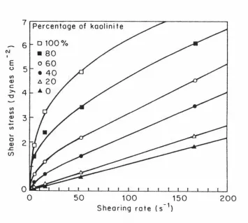
the concentration of suspended particles. On the other hand, non-newtonian fluids

exhibit a dynamic viscosity which varies with shear or strain rate (Figure 2.3). For

example, fluids containing clay minerals in suspension are known to diverge from the

newtonian response for clay concentrations above a certain value and for a proportion

(21)

Non-newtonian rheologies are typical of many natural flows, such as water-saturated muds

(fluid muds), while this non-newtonian response plays an important role in the

[image:21.595.109.488.156.513.2]

processes of slumping, sliding and avalanching.

Figure 2.3 Shear stress plotted against shear rate for materials of different rheological behaviour (Leeder, 1999).

Based on the behaviour of substances under shear, several types of rheological

response can be distinguished (Figure 2.3). In pseudoplastic (non-newtonian)

materials the dynamic viscosity (µ) is high at low shear rates but decreases with

increasing shear rate up to a constant value. Such substances are also known as

shear-thinning, e.g. muddy fluids, showing a structure of interacting clay particles that

increase the fluid’s overall resistance to the flow. As the shear rate in a muddy fluid

increases, this structure is gradually destroyed and then the shear-thinning behaviour

(22)

viscosity (µ) increases with the shear rate. This type of rheological response is

common in some polymer suspensions. Bingham plastic substances show a

Newtonian behaviour, as the dynamic viscosity remains constant under increasing

shear rates. However, an initial shear stress, termed as the ‘yield stress’, must be

applied before strain occurs. The Bingham yield stress arises due to residual effect of

particle interaction and is related to the magnitude of the attraction among the

particles. Examples of natural flows showing plastic behaviour are lava and debris

flows. In such flows, a finite yield strength allows morphological features like levees,

flow snouts and flow wrinkles to be preserved during flow and after motion has

[image:22.595.121.476.303.622.2]

stopped, while particle settling is likely to be hindered or even impossible.

Figure 2.4 Rheological behaviour of quartz/kaolinite mixtures in suspension for varying percentages of kaolinite (Volumetric concentration is 0.2%) (James & Williams, 1982).

Some examples of geophysical flows, driven by various mechanisms and showing a

Newtonian-flow type are the following: a) surface water flows in river and delta

(23)

driven by wind shear, pressure gradients and Coriolis force d) deep ocean currents

driven by gravity acting on density contrasts, which are caused by salinity differences

and differential heating or cooling. On the other hand, mass flows of sediment and

water exhibit density contrasts due to the presence of suspended sediments, e.g. debris

flows and turbidity currents. Such flows are also driven by gravity forces but show a

flow type which varies from non-newtonian to newtonian (Leeder, 1999).

2.3 Newton’s laws in Fluid Dynamics

Newton’s laws of motion are very important in fluid dynamics, as they govern the

motion of all fluids. According to the first law, known also as the ‘principle of

inertia’, a constant mass of a fluid will remain still or continue to move along the

same direction at a constant velocity, provided that none externally applied force is

acting on this mass.

In the second Newton’s law it is stated that the magnitude of an externally applied

force equals to the rate of change of momentum that takes place along the direction of

the force. Therefore, the magnitude of a force can be calculated according to the

produced acceleration or deceleration. The momentum per unit volume of a fluid of a

constant density is ρu, thus the rate of change of this momentum is:

dt du

F =ρ / Eq 2.4

(24)

Finally, the third law states that the force exerted by one fluid/solid mass on another

fluid/solid mass is equal and opposite to the force it experiences from the other mass.

This law is applied to flows where velocity gradients are developed, e.g. within

boundary layers. Then the shear stress exerted on the top surface of a thin fluid layer

is opposed by an equal stress exerted below. Even in ideal flows, where frictional

forces grown at solid boundaries are assumed to be negligible, Newton’s third law

applies and the fluid force is acted upon by an equal and opposite reactive force from

the bed. However, in natural flows the movement of a fluid over a bed is strongly

affected by frictional drag developed within a relatively narrow zone, the boundary

layer (§2.4). In this zone the flow speed is decreased relative to the current speed

away from the solid boundary.

2.4 The dynamics of the flow

Various aspects in fluid dynamics are approached by considering ‘ideal’ flows of

inviscid fluids. Such ‘ideal’ fluids are characterized by zero viscosity (µ=0) and

they don’t show any resistance to the flow. Consequently, they don’t develop

frictional forces on their boundaries. However, this does not hold true in the case of

natural flows of non-ideal fluids. Whenever a real fluid moves over a solid boundary,

frictional drag forces are developed, decreasing the velocity within a narrow zone

close to the boundary. The fluid molecules in immediate contact with the boundary,

attach to it and form an adsorbed layer which is stationary relative to the free-stream

flow. Obviously, the flow velocity decreases from its free value away from the

boundary to almost zero at the boundary. Such zones of flow retardation are known as

boundary layers (Figure 2.5). A boundary layer is formed every time a real fluid

moves over a sediment-substrate or through a channel or around a fixed object or even

when an object is moving relative to a stationary fluid mass (e.g. settling of particles).

The flow velocity increases with the distance above the boundary, until it reaches its

free-stream value. A boundary layer is characterized by the presence of velocity

(25)

If we consider a fluid moving over a flat plate with a uniform velocity u_max then a boundary layer will be formed, thickening downstream from the leading edge (Figure

2.5). Three sections can be distinguished. In the initial part the flow will remain

laminar over some distance from the edge and the thickness (δ ) of the boundary layer

will increase with the square root of the distance x from the edge (Schlichting,

[image:25.595.90.503.222.468.2]

1951):

Figure 2.5 The boundary layer developed over a flat plate (Leeder, 1999).

2 / 1

max

5 _

  

 

=

u x

ρ µ

δ Eq 2.5

where µ is the dynamic viscosity and ρ is the fluid density. Within the laminar

boundary layer the time-averaged velocity at a fixed point will be exactly the same as

the instantaneous velocity at that point. The velocity distribution is described by:

) 2 (

2

δ µ

τ y

y

(26)

where u is the flow speed at height y above the boundary, τ is the shear stress at the boundary, µ the viscosity and δ the boundary layer thickness (Leeder, 1999).

Setting y=δ and u=u_max, where u_max is the flow velocityoutside the boundary layer, Eq 2.6 yields:

δ µ

τ = 2 umax Eq 2.7

Eq 2.7 shows that the shear stresses associated with laminar boundary layers are very

small. The thickness of the laminar boundary layer continues to increase with the

distance along the plate so that at a certain distance the motion is not stable any more

and starts to be turbulent. Then fluid eddies start to develop and the boundary layer

becomes transitional. Finally, beyond some critical distance the inertial forces will

dominate and the flow will become fully turbulent. The velocity distribution within

the turbulent boundary layer is given by:

n y u

u

) (

max δ

= Eq 2.8

where u is the local time-averaged velocity. The exponent n varies from about 1/5

near transition to about 1/7 further downstream (Leeder, 1999).

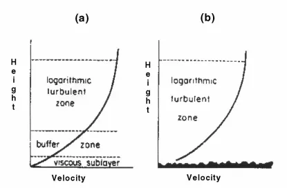
The turbulent boundary layer formed over a smooth boundary can be divided in three

regions (Figure 2.6). The viscous sublayer is a thin zone, lying immediately adjacent

to the boundary where the flow velocity is low. The velocity gradient within the

viscous sublayer is almost constant. The shear stress is controlled by dynamic

viscosity µ and is given by Newton’s viscous stress equation (Eq 2.2,

dy du

µ

τ = ) or

µ τ µ

τ dy y

u=

∫

1 = Eq 2.9

(27)

*

/ 5 . 11

δ′= ν u Eq 2.10

The quantity u , is the _* shear or friction velocity and has the dimensions of velocity. It is defined as:

ρ τ

* =

u Eq 2.11

[image:27.595.89.504.355.627.2]

where τ is the shear stress exerted on the boundary by the fluid and ρ is the fluid density. The shear velocity u_* is directly proportional to the rate of increase of fluid velocity with height, and it is therefore proportional to the slope of velocity distribution curve.

Figure 2.6 Turbulent boundary layers formed above smooth (a) and rough (b) boundaries (Komar, 1976).

(28)

the viscous transfer. Based on the assumption that du /dy decreases with the distance

from the boundary, we get:

y dy

du 1

∝ or dy

y k

u=

∫

1 or

c y k

u= log_e + Eq 2.12

where k and c are constants. A fuller form of the above equation is called the Prandtl’s ‘law of the wall’ and provides the variation of streamwise velocity with height in turbulent flows (Coleman, 1981). The lower part of the logarithmic layer merges into the linear viscous sublayer via a narrow zone, which is known as the buffer layer (or equilibrium layer). In this zone the viscous and turbulent transfer of momentum are comparable. In Figure 2.6 the turbulent boundary layers developed over a smooth and a rough boundary are depicted. The presence of boundary roughness disrupts the viscous sublayer and the logarithmic zone extends to the boundary.

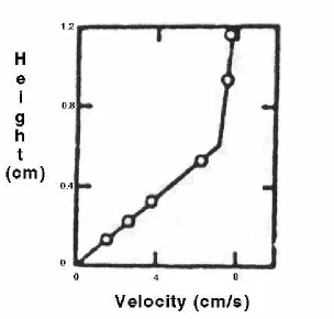
In Figure 2.7 the mean flow velocity measured across a smooth boundary, is plotted against height above the sea-bottom. The upper line, corresponding to the logarithmic sublayer, is a least-squares fit of a logarithmic form to flow velocities measured at 1 cm above bottom. The lower part of the plot represents a linear fit to flow velocities measured at heights below 0.6 cm and corresponds to the viscous sublayer.

The flow boundary roughness can be defined by comparing the thickness of the viscous sublayer of turbulent flows to the size of sediment grains or boundary irregularities. Smooth boundaries are those, whose roughness elements of sedimentary particles are completely enclosed within the viscous sublayer and consequently they develop only viscous forces. When the particles project through the sublayer, they favour the growth of eddies and the boundary is said to be transitional or rough, depending on the degree of penetration.

(29)

laminar one. The turbulent viscosity is not a constant, so the shear stress has generally

[image:29.595.146.450.134.424.2]

to be calculated empirically.

Figure 2.7 Mean flow velocity versus height above the sea-bed (Caldwell, 1979).

2.5 Reynolds number and flow regimes

Osborne Reynolds observed in 1883 that two distinct flow types can be distinguished:

laminar or viscous flow at low flow velocities and turbulent flow at high flow

velocities. Considering fluids of different viscosity flowing through pipes of various

diameters, the change from laminar to turbulent flow was found to occur at a fixed

value of a dimensionless parameter, known as the Reynolds number (Re). It is:

ν ud =

Re Eq 2.13

(30)

is substituted by the hydraulic radius of the channel which equals the mean flow depth

if the channel width is much greater than water depth.

The Reynolds number is a manifestation of the effect of viscous forces relative to

inertial forces acting on a fluid. When Re is low, then viscous forces dominate and the flow is said to be laminar. A laminar flow is stable and the fluid particles move along definite straight trajectories. When Re is high, then inertial forces dominate and the flow is turbulent. A turbulent flow is characterised by irregularities or disturbances, which lead to the formation of eddies, diffusing across the flow as well as moving in the mean direction of the flow. In such a flow the fluid particles move along random fluctuating trajectories. The turbulent flow can be considered as a complex motion where random velocity fluctuations (due to the motion of eddies) are superimposed on the average motion of translation. The turbulent eddies can transfer momentum normal to the flow boundary at a rate much higher than the molecular transfer in laminar flows. In this case an additional resistance to the flow arises, expressed by the eddy viscosity, which is not constant for a given fluid and temperature. As an example, many water flows in rivers are turbulent. The change from laminar to turbulent flow conditions occurs progressively, over a range of values of Re . Within this range the flow is characterised as transitional. In open-channel flows, the transitional range of Re values is between 500 and 2000 (Leeder, 1999). For Reynolds numbers higher than 500, instabilities develop within the flow, which gradually becomes fully turbulent. The critical value of Re depends to some extent on the number of irregularities and obstacles, present on the channel bottom. For example, an open channel flow over a smooth bottom could remain laminar for Re >500 and up to Re = 2000. However, in natural channels with a rough bottom the critical value of Re is low, as the bottom irregularities favour the growth of turbulent eddies and the transition to turbulent conditions. In natural flows the laminar conditions are very rarely observed, as turbulent flows dominate. The only exception is very close to a sufficiently smooth boundary, where the viscous sublayer can develop with viscous stresses dominating over turbulent stresses.

(31)

ν s

k u_* *

Re = Eq 2.14

where u_* is the shear velocity and k_s is the grain effective roughness height (Allen, 1985). Combination of Eq 2.10 with Eq 2.14 gives:

δ

5 . 11 Re_*

′

= ks Eq 2.15

The grain Reynolds number (Re ) is proportional to the ratio of the grain effective _* roughness height (k ) to the thickness of the viscous sublayer (_s δ′). Thus, it provides a measure of grain protrusion through the viscous sublayer, which is further used in defining whether turbulent eddies are produced. When Re is less than 5, the bottom _* roughness has a negligible effect on the flow and the bottom is considered as smooth. For Re higher than 70, the viscous sublayer is completely disrupted and the bottom _* is considered to be rough. In such a case, viscosity appears to have a low effect on the mean flow. The change from smooth to rough boundary conditions occurs within the transition region 5<Re <70 (Schlichting, 1979). _*

2.6 Energy losses and friction factors

According to Newton’s second law (see §2.3) when a fluid is moving over a solid boundary with a constant velocity then frictional forces arising from viscosity and turbulence, act on fluid elements in a direction opposing the fluid motion. Thus, in a steady flow of a non-ideal fluid there will be a continuous loss of energy due to friction and subsequently the total energy of the flow will decrease along a streamline because of energy dissipation.

(32)

whenever a fluid mass moves past a bend of the flow-channel or constricts or

expands. Besides, due to sediment transport a mobile bed layer (bedload) is formed,

causing further energy loss. All the previous forms of energy losses can be included in

a synoptic friction coefficient for a particular flow. The friction factor f is

dimensionless and is given by the ratio of shear stress τ , exerted by the flow on the

surface of a solid boundary to the mean kinetic energy per unit volume, or:

) 2 1 ( 2 u f ρ

τ = Eq 2.16

Eq 2.16is known as the ‘quadratic stress law’. The coefficient of proportionality f

is called drag coefficient and expresses in a non-dimensional way the drag, which is exerted by the moving fluid to the solid stationary bed. Friction coefficients describe the total drag, including form and skin friction. Depending on how the proportionality factor is defined, the quadratic stress law appears in different forms. Regarding an object, which is moving within a stationary enclosing fluid, Eq 2.16 is written as:

) 2 1 ( u2 c_D ρ

τ = Eq 2.17

where cD is the drag coefficient. For channelized flows it is:

) 2 1 ( 4 2 u f _ρ

τ = Eq 2.18

where the constant of proportionality is known as the Darcy-Weisbach friction coefficient.

(33)

diameter to flow thickness. In the same way, the drag coefficient in a fully developed

turbulent flow through a pipe depends on the wall roughness of the pipe (Nikuradse,

1950). Additionally, the bed drag coefficient can vary over a mobile sea bed

(McCave, 1973) or due to bed-form development (Dyer, 1980) or in response to

changes in the flow regime (Sternberg, 1968). The drag coefficient of a fixed bed is

also known to vary, either with the direction of tidal current relative to bed forms

(McCave, 1973) or due to the existence of waves, which interact nonlinearly with the

steady flow within the wave boundary layer (Grant and Madsen, 1979; Green et al.,

1990). Finally, the presence of saltating particles which act as a momentum sink, can

differentiate the drag coefficient (Smith and McClean, 1977; Grant and Madsen,

1982), while the suspended particulate matter within a flow can cause a stable

stratification of the boundary layer, thus considerably affect the observed values of

drag coefficient (Huntley et al., 1994; Green and McCave, 1995).

The drag coefficient is considered a very important parameter, used in the evaluation

of the shear stress induced on the sea bottom by the overlying flow. For example, in

the quadratic stress law if the value of the drag coefficient at a fixed height above sea

bed is accurately known, then the unknown shear stress can be estimated from a

single measure of flow velocity at the considered height. This takes away the need for

obtaining the complete velocity profile and then determining the shear stress using the

law of the wall (Sternberg, 1968; Yalin, 1972). Sternberg (1968, 1972) calculated an

average value for the drag coefficient for fully developed turbulent flows, through

numerous measurements of velocity profiles in Puget Sound, Washington. He

proposed:

3

100 3.1 10

−

× = D

C Eq 2.19

(34)

into account, although they provide higher resistance to the flow and so affect the

value of C_D₁₀₀. The second limitation is that the use of a mean constant C_D₁₀₀

assumes the absence of suspended sediment in the flow, which is not usually the case.

Consequently, the generalised use of a constant value of drag coefficient, irrespective

of flow strength, the presence of bedforms and suspended particulate matter could

lead to erroneous shear stress estimations.

The friction coefficients are generally determined experimentally. In particular, the

calculation of the bed drag coefficient in natural marine settings is difficult, as it is

based on some conventionally used methods. The most common method is the

velocity profile method, which requires velocity measurements on a vertical array

within the boundary layer. Large sources of error are involved in this method,

including noise in velocity measurements, inaccurate knowledge of the position of

measurements relative to the bed, etc. Other conventional methods include the use of

hot-film probes, which relate the heat dissipation directly to shear stress (Graham et

al., 1992) and the measurement of Reynolds stresses near the boundary (Soulsby,

1983). This method is very sensitive to sensor misalignment and can give large errors

of 156 % per degree of misalignment in wave-dominated environments (Soulsby and

Humphrey, 1989). It is concluded that the routinely used methods of determining the

bed drag coefficient show various problems when used in field applications and their

use is based on assumptions, which should be carefully considered under certain

circumstances.

2.7 The boundary shear stress - measurement techniques

In sediment transport investigations and particularly in predictions of movement

initiation of sediment particles, a key parameter is the bottom shear stress (τ ) exerted

by the fluid which is moving over a sandy or cohesive substrate. Therefore, in such

investigations the objective is the estimation of the fluid shear stress on the boundary

and this can be achieved by several methods in the case of an assumed steady

two-dimensional turbulent flow (in an open channel). The methods include the Velocity

Profile method (Bowden, 1962; Sternberg, 1968; Yalin, 1972; Li & Gust, 2000) and

(35)

1983), which are considered as the most commonly used techniques. All of the

conventionally used methods show some advantages but at the same time include

sources of error and/or require measurement techniques which are not simple, hence

they are not characterised by the ease of application.

In the velocity profile method, the mean flow speed is measured at a few levels within

the water column. Assuming a logarithmic profile, the mean flow speed (u ) at a z

given distance (z ) above the sea-bottom is related to the bottom shear stress by the

Karman-Prandtl equation:         = o z z z k u

u *ln Eq 2.20

where u_* is the friction velocity

(

τ ρ

)

1/2, k is von Karman’s constant and z_o is the roughness length (generally increasing with the boundary roughness). The measured

values of u are plotted against z on a semi-logarithmic scale and the slope of the z

velocity profile gives the boundary shear stress (τ ). The application of this method is

based on the assumption of a steady flow and a constant shear stress above the

boundary. Consequently, a large scatter in the values of u_* and z_o can be obtained and this can be attributed to many reasons, including flow unsteadiness, noisy velocity

measurements, inaccurate determination of the height of velocity measurements,

varying bottom roughness. In addition, the drag form (if present) is not considered as

well as the presence of suspended sediments, which change the value of k (Sternberg, 1972).

According to Quadratic Stress Law equation, the boundary shear stress is proportional

to the fluid density and the square of the mean flow speed measured at a distance z

from the boundary. Considering the bed drag coefficient C_D_z at height z as the coefficient of proportionality, the Quadratic Stress Law is given by:

2 z z D u C ρ

(36)

Eq 2.21relates the shear stress at the boundary to a single measured value of the flow

velocity within the boundary layer. The main advantage of the method is the

simplicity in its application. However, the use of the quadratic stress law is based on a

logarithmic velocity distribution, which is not always the case. For example, it has

been demonstrated that during various tidal flows, logarithmic velocity profiles

occurred between 62% and 100% of the time (Sternberg, 1968). Consequently, a

certain degree of uncertainty is introduced in the use of the quadratic stress law

method when it is applied in shear stress estimations.

Furthermore, the boundary shear stress τ can be estimated using the ‘eddy correlation

method’ (Soulsby, 1983), by measuring directly the Reynolds stresses in the constant

stress layer of the flow:

const u′ ′= −

= ρ υ

τ Eq 2.22

where u′ is the longitudinal fluctuating component of velocity and υ' is the vertical fluctuating component of velocity. The overbar in Eq 2.22 indicates the mean value. This method is particularly sensitive to sensor misalignment and can give errors up to 156 percent per degree of misalignment under specific conditions (Soulsby and Humphrey, 1989). Although the method assumes the existence of a constant stress layer, it is known that the shear stress can also fluctuate with the distance from the boundary. In hydraulically smooth flows, the ‘gradient method’ is used for accurate determination of the bottom shear stress by mean flow measurements within the viscous sublayer:

2 1

* ( du dz)

u = ν Eq 2.23

In flume experiments the ‘energy slope method’ is often used for shear stress estimation:

gRS

ρ

(37)

where g is the gravity acceleration, R is the hydraulic radius of the flume, and S is the surface slope. Shear stress values calculated by Eq 2.22 and Eq 2.23 are local

boundary stresses, while that obtained by Eq 2.24 is a bottom shear stress averaged

over the entire flume. The latter value is not as accurate as the local stresses because it

is affected by: the non uniform distribution of τ along the flume walls, the side-wall

effects and the secondary currents (§ 3.3 ).

2.8 Sediment transport modes

The motion of the transported sediment particles normally takes place in three distinct

modes: rolling and/or sliding motion, saltating motion and motion in suspension. It is

known that when the value of the bed shear stress is just above the critical value for

motion initiation, then the sediment particles are removed from their resting position

and erosion starts to take place. The particles start rolling and/or sliding but they

remain nearly always in contact with the bed. As the exerted bed shear stress

increases, the sediment particles start making a leaping motion (saltation). The

sediment grains moving along a bed by rolling, sliding and saltation constitute what is

known as bedload. Finally, when the vertical component of the flow velocity

becomes comparable to the particle settling velocity, then the particles are lifted to a

level within the water column at which the upward turbulent forces can balance their

submerged weight, so the sediment particles can go into suspension (Francis, 1973).

Such moving particles form the suspended load and practically move with the same

speed as the speed of the carrier flow. The fine uniformly dispersed particles are

responsible for the turbidity of the flow. The suspended load also includes the

washload, which is a broad term describing the clay-size particles brought into

suspension more or less permanently.

Bedload and suspended load transport can occur at the same time within the same

current, however the limit between these two modes of transport is not strictly

defined. The relative percentage of transported sediment grains, moving in three

different modes is shown in Figure 2.8 as a function of the transport stage. The latter

is defined as the ratio

c u

(38)

velocity, required for the initiation of particle motion. It is obvious that near the

threshold the rolling motion dominates over saltation and suspension. However, at

high values of the ratio u_*/u_*_c the proportion of rolling particles decreases very steeply, while the proportion of suspended particles increases.

Additionally, experimental work has shown that bedload transport could be observed both in laminar and turbulent flows (Bagnold, 1955). Regarding the forces acting on transported sediment grains, bedload can be defined as the portion of grains whose immersed weight is balanced by an upward intergranular force, arising due to grain shearing over a solid bed (Bagnold, 1966). This does not apply to the suspended load transport, occurring only in turbulent flows. In such flows the fine suspended particles are evenly distributed within the whole water column and the collisions among them are very rare, so intergranular forces supporting the suspended load cannot be developed. In this case, the suspended load is supported by forces developed due to fluid turbulence.

(39)

2.8.1 Cohesive sediment transport

The previous considerations were based on the assumption that the transported

sediments were relatively coarse cohesionless grains, moving as separate particles.

However, if clay minerals, clay mineral flocs and cohesive clay beds are involved,

then the situation is different, because the clay solids in transport do not behave as

separate individual particles but interact electrostatically, showing a certain degree of

cohesion.

Clay size particles are platelike and carry a negative electric charge on their surfaces,

caused by isomorphous substitution in their lattices. The presence of a saline fluid,

e.g. seawater, causes the negative charges to be neutralized and subsequently the

approaching clay particles do not repel any more, allowing London-van der Waals

molecular forces to establish attraction between individual clay platelets Such

attractive forces can counteract the electrostatic repulsive forces. In this case, the

process of flocculation takes place, where larger aggregates of grains are formed

from many individual platelets. On the contrary, in fresh water (e.g. in river water) the

electrostatic repulsive forces normally dominate and the flocculation process is

inhibited. Consequently, flocculation is more effective in saline water. The attractive

London-van der Waals forces are known to be inversely proportional to the square of

the distance between the clay platelets. Therefore, the formation of flocs depends on

intergranular collisions, which bring the clay platelets in very close proximity. The

concentration of suspended particles is also important, as in dense suspensions the

probability of particles brought very close together is high. Temperature variations

also affect the flocculation process. At high temperatures the thermal motion of ions is

more intense and the repulsive forces become larger, so the formation of aggregations

is prevented. Additionally, the presence of organic material on the particles

encourages organic binding, which leads to larger and stronger flocculates

(Whitehouse et al., 1960). The formation of aggregates is known to be a reversible

phenomenon, which means that if sediment flocs are put in fresh water, then they will

be subject to disaggregation processes, particularly enhanced by turbulent shearing

(Jeffrey, 1982; van Leussen, 1997). An important problem involved in the study of

flocculated mud aggregates is the difficulty of measuring the floc size from fluid

(40)

the flocs and disaggregation. In order to get over such problems, a number of in situ

techniques have been developed (McCave, 1979; Eisma et al., 1997). For example,

Owen (1971) has developed a tube for measuring the fall velocity under laboratory

conditions closely resembling the natural state. Holographic techniques have also

been used successfully in the open sea for in situ measurements of the flocs size and

their fall velocity (Carder et al., 1982).

It is known that the flocculation process depends on clay particle concentration:

increased concentration leads to increased number of interparticle collisions and

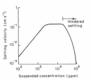
therefore, to increased flocculation rate. As expected, the settling velocity of the

grown aggregates will increase with increasing concentration. However, after the

settling velocity obtains a peak value, a further increase in particle concentration

causes a decrease in settling velocity due to the effect of ‘hindered settling’

phenomenon (Figure 2.9). This means that both the settling flocs and single particles,

moving downwards within the dense suspension displace a certain fluid mass, which

in turn moves upwards, preventing further settling. The flocculation rate also

increases with increasing salinity and subsequently a given fall velocity of flocculates

will be observed at a lower concentration if the ambient fluid is more saline (Owen

1970).

The reduced settling velocity of flocculates in dense suspensions due to ‘hindered

settling’ has been described by Maude & Whitmore (1958). The proposed formula

was:

m o

s w C

w = (1− ) Eq 2.25

where w is the fall velocity of a particle in a suspension of other falling particles, _s w _o

is the fall velocity of a single particle in an otherwise particle-free fluid, C is the volume concentration of particles in the suspension, and m is a function of particle size and shape. For small particles m is equal to 4.65, while for large particles

32 . 2

=

(41)

[image:41.595.138.462.74.355.2]

Figure 2.9 The settling velocity plotted against suspended sediment concentration for mud from the Severn Estuary (Odd, 1982).

In certain environments flocculation becomes a very important process, e.g. at estuary

heads, where fresh water is mixed with seawater by turbulent eddies. The mixing of

fresh and salt water causes estuarine circulation driven by density gradients. It has

been observed that the combined effect of the flocculation process and hindered

settling can lead to the development of distinct layers of high suspended sediment

concentration in great proximity to the sea bottom (Figure 2.10).

This is particularly common in tidal-dominated estuaries (Kirby and Parker, 1983). In

such environments silt- and sand-sized particles combine in larger aggregates, which

then settle and form large areas of mobile and stationary mud suspensions (fluid

muds) of very high densities. Mobile suspensions can potentially flow along the

bottom without mixing considerably with the overlying flow because of the high

density contrast. Additionally, they can move freely downslope as density currents

under the influence of gravity. Stationary fluid muds show high densities (up to 200

g/l) and can be rapidly deposited at a thickness of 2-4 m (Dyer, 1986). They are

(42)

the sediment concentration is much lower. Such suspensions do not move

horizontally, however, gradual settling could occur. Sediment cores obtained through

stationary fluid muds reveal structureless muddy silts with occasional thin sandy

laminae (Kirby and Parker, 1983), while sonar records show sharp upper surfaces of

[image:42.595.91.504.190.444.2]

stationary suspensions.

Figure 2.10 Concentration and velocity profiles with associated sediment fluxes. The velocity profile represents wave motion. (Mehta & Li, 1998)

The erosion of a muddy bed by a flow will generally occur when the bed shear stress

exceeds the local critical shear resistance. However, the threshold conditions for

entrainment of mud are not simply a function of grain size, but depend on various

parameters, like clay mineralogy, chemical composition of fluid, state of fluid flow,

organic content and previous depositional history. For example, consolidation of

deposited muddy beds is very important, because it causes an increased cohesiveness,

hence increased erosion resistance with depth. This results in high surface erodibility

of muddy beds, which is followed by stability at a greater depth. Additionally, the

presence of surface algal films and coatings on many marine deposited muds exhibits

(43)

3 Sediment-laden flows

In this chapter a general review on studies concerning sediment-laden flows is

presented, including basic observations and experimental results. Emphasis is placed

on experimental investigations, conducted with the use of artificial channels

(laboratory flumes) and in particular the annular flumes. The subchapter 3.1 consists

of some background information on suspension flows, including specific difficulties

introduced by the presence of cohesive suspended solids within a flow. The

subchapter 3.2 refers to the drag reduction phenomenon, exhibited by natural and

laboratory turbid flows. In subchapter 3.3 a brief overview is given on the use of

laboratory and in situ annular flumes by various researchers, who studied

sediment-laden flows.

3.1 Complications introduced by the transported solid phase

Most of the natural flows are not homogenous because they carry a certain amount of

suspended load. If the suspended material is cohesionless, then the flow can be

considered as Newtonian. In this case, only Von Karman’s constant k and kinematic viscosity ν are changed (Hunt, 1954). If the suspended sediments are cohesive, then

Bingham-like behaviour occurs, with an increase in apparent bulk viscosity directly

related to the amount of transported clay and shear rate (Wan, 1982). In other words,

we have a two-phase system which behaves as a viscous non-Newtonian fluid (Wood

et al., 1995; Metzner, 1961). The latter was proven experimentally by Gust (1976),

who used a dilute seawater-clay suspension in a laboratory channel and found that the

applicability of the universal ‘law of the wall’ (see §2.4) was not correct in this

(44)

It is known that the friction velocity (Eq 2.11) u_* =(τ/ρ)1/2 (τ = bottom stress, ρ=

fluid density) is a fundamental parameter, used in the investigation of erosion and

sedimentation processes of geophysical boundary layers. It can be estimated from

mean streamwise velocity measurements in the logarithmic layer of the turbulent

boundary layer. For hydraulically smooth flows of Newtonian fluids the friction

velocity u_* is calculated by solving the equation:

1 *

* 1/ ln( / )

/u k yu C

u = ν + Eq 3.1

where u= local mean streamwise velocity, y= vertical coordinate, and ν= kinematic viscosity. Eq 3.1 is known as the ‘Law of the Wall’ and with k=0.4 and C₁=5.5 is valid for equilibrium boundary layers of fully developed turbulent Newtonian smooth

flows. Within the range of validity, the values of k and C₁ slightly depend on Reynolds number (Tennekes and Lumley, 1971; Tennekes, 1973). Therefore, the

values of the critical friction velocity u_*_crit and erosion rates obtained under the assumption of a Newtonian flow structure should be reviewed in the case of

sediment-laden flows. This means that the universal law of the wall is not valid for turbulent

two-phase flows.

Gust (1976) in his previously mentioned experiment simulated a tidal flow under

highly controlled laboratory conditions, using an artificial channel coated with mud

and unfiltered seawater from the North Sea. He obtained mean streamwise velocity

profiles for Reynolds numbers between 5400 and 27800 (i.e. non-eroding and eroding

flow rates) in order to investigate the boundary layer structure of the seawater-clay

suspension down into the viscous sublayer. Although the distributions of

concentration showed no substantial increase towards the wall, he found that the

thickness of the viscous sublayer (which was normally of the order of 1 mm) was

increased by up to a factor of 5 compared with Newtonian flows under the same

conditions. Additionally, the friction velocity u_* determined by the ‘gradient method’ (Eq 2.23) in the viscous sublayer was reduced up to 40% in suspension flows. Gust

(45)

factor f , which is a function of Reynolds number Re and clay suspension parameters causing the reduction in the friction velocity u . It is: _*

2

* )

(

8 u U

f = Eq 3.2

where U is the mean channel flow velocity, and:

ν R U

4

Re= Eq 3.3

where R is the mean hydraulic radius. In Figure 3.1the data for the clay suspension show a downward shift from the clear water values, demonstrating the occurrence of the drag reduction phenomenon which is explained in §3.2.