Integrated design of discrete time controller for an active suspension system

Integrated design of discrete-time controller for an active suspension system

Dina Shona Laila

Department of Electrical and Electronic Engineering,

The University of Melbourne, Parkville 3010, Victoria,

Australia.

[email protected]

Abstract— A novel approach to solve a stabilization problem of an active suspension system using a quarter car model is presented. We apply a combination of our results for the framework of the approximate based direct discrete-time design and the Euler based discrete-time backstepping technique. This stabilization problem is very interesting since utilizing a simple quadratic Lyapunov function brings the system into a LaSalle type stability, which makes the design more complicated. To handle this problem, we use our result on changing supply rates lemma for LaSalle type stability condition, to construct a composite Lyapunov function that can be used for the design within our framework.

I. INTRODUCTION

Most control systems nowadays are sampled-data in na-ture. A controller is usually implemented digitally and it is inter-connected with a continuous-time plant via ADC and DAC. In this paper, we study the problem of stabilizing an active suspension system, which is used to enable a car to run smoothly on a rough road for comfortable driving. Presently, active suspension systems are controlled using a hydraulic controller. In view of space limitation in a vehicle, it is most appropriate to use digital device to control the active suspension system, as it requires much less space. Since the active suspension module itself is a mechanical - therefore analog - plant, designing a digital controller for this system is a sampled-data system design.

Recently, a general uni£ed framework for controller design based on approximate discrete-time models was presented in [10] and further generalized in [7] for the input to state stabi-lization problem. In particular, the results provide suf£cient conditions for the continuous-time plant model, the controller and the approximate discrete-time model, to guarantee that the controller input-to-state stabilizes the exact discrete-time plant model, provided it stabilizes the approximate discrete-time plant model.

We design a discrete-time controller to asymptotically stabilize the active suspension system, using the Euler based backstepping technique [9]. Backstepping is a popular tech-nique in nonlinear control design (see [4]). It is then shown that the Euler based discrete-time controller outperforms the emulation controller. This active suspension design problem is very interesting and motivating since the system enjoys a LaSalle type stability when using a simple quadratic Lya-punov function. In [3], where continuous-time stabilization for the same system was considered, stability analysis was done using LaSalle’s invariance principle. Unfortunately,

LaSalle’s invariance principle is in most cases not applicable when approximate based discrete-time design is used, since semiglobal type of stability is usually achieved. In this situ-ation, we apply our result from [6] to construct a composite Lyapunov function that can be used to characterize stability property of the system.

II. PRELIMINARIES

The set of real and natural numbers (including 0) are denoted respectively by RandN. SN denotes the class of smooth nondecreasing functions q : R≥0 → R≥0, which

satisfyq(t)>0for all t >0. A function γ:R≥0→R≥0 is

of classGif it is continuous, nondecreasing and zero at zero. It is of classKif it is of classGand strictly increasing; and it is of classK∞if it is of classKand unbounded. Functions of classK∞are invertible. A functionβ:R≥0×R≥0→R≥0is

of classKLifβ(·, t)is of classKfor eacht≥0andβ(s,·)

is decreasing to zero for each s > 0. Given two functions

α(·)andγ(·), we denote their composition and multiplication respectively asα◦γ(·)andα(·)·γ(·).

We consider a parameterized family of discrete-time non-linear systems of the following form:

x(k+ 1) =FT(x(k), u(k)), y(k) =h(x(k)), (1)

where x∈_Rn_{, u∈R}m_{, y ∈ R}l _{are respectively the state,}

input and output of the system. Note that the inputucan be a control signal or an exogenous disturbance. It is assumed that FT is well de£ned for all x, u and suf£ciently small

T, FT(0,0) = 0for allT for whichFT is de£ned, h(0) = 0 and FT and h are continuous. T > 0 is the sampling

period, which parameterizes the system and can be arbitrarily assigned. The following de£nitions are used to state results presented later in this section.

De£nition 2.1: The system (1) is semiglobally practically

input-output to state stable (SP-IOSS), if there exist functions

α, α, α∈ K∞, and λ, σ∈ G, and for any triple of strictly positive real numbers(∆x,∆u,ν), there existsT∗>0and

for allT ∈(0, T∗_{)there exists a smooth functionV}

T :Rn→ R≥0 such that for all |x| ≤ ∆x, |u| ≤ ∆u the following

holds:

α(|x|)≤VT(x)≤α(|x|) (2)

VT(FT(x, u))−VT(x)≤ −T α(|x|) +T λ(|y|)

The functionVT is called a SP-IOSS Lyapunov function. If

the system is SP-IOSS withλ= 0, we say that the system is semiglobally practically input to state stable (SP-ISS) and

VT is called a SP-ISS Lyapunov function. If λ= 0and the

system (1) is an input-free system (σ = 0), the system is semiglobally practically asymptotically stable (SP-AS) and

VT is called a AS Lyapunov function. Moreover, for

SP-ISS, if the argument ofα(·)is the norm of the outputy, which consists of only partial states, we have semiglobal practical

quasi ISS (SP-qISS). ¥

De£nition 2.2: [9] LetT >ˆ 0 be given and for each T ∈

(0,Tˆ) let the functionsVT :Rn →R≥0 anduT :Rn →R

be de£ned. We say that the pair(uT, VT)is a semiglobally

practically asymptotically (SPA) stabilizing pair for FT if

there exist α, α,α∈ K∞, such that for any pair of strictly positive real numbers (∆, ν) there exists a triple of strictly positive real numbers (T∗_{, L, M), with T}∗ _≤Tˆ_{, such that} for allx, z∈_Rn _{withmax{|x|,|z|} ≤∆, andT ∈(0, T}∗₎ we have:

α(|x|)≤VT(x)≤α(|x|) (4)

VT(FT(x, u))−VT(x)≤ −T α(|x|) +T ν. (5)

|VT(x)−VT(z)| ≤L|x−z| (6)

|uT(x)| ≤M . (7)

¥

III. DESIGN TOOLS

A. Framework for approximate based direct discrete-time design

In this subsection we present a result from [7] on input to state stabilization via approximate discrete-time models. Consider a continuous-time nonlinear plant

˙

x(t) =f(x(t), u(t), w(t)), y(t) =h(x(t)), (8)

where x ∈ _Rnx_{, u ∈}

Rm_{, w ∈ R}p _{and y ∈ R}l _are

respectively the state, control input, disturbance and output. We assume that for any given x0, u(·) and w(·) the

differential equation in (8) has a unique solution de£ned on its maximal interval of existence[0, tmax). This may be guaranteed, for instance, by requiringf in (8) to be locally Lipschitz. The control is taken to be a piecewise constant signalu(t) =u(kT) =:u(k), ∀t∈[kT,(k+ 1)T),k∈_N, whereT >0is the sampling period, and we suppose that the disturbance w(·)is constant during sampling intervals, that isw(t) =w(k),∀t∈[kT,(k+ 1)T). We assume that some combination (output) or all of the states (x(k) :=x(kT)) are available at sampling instantkT, k∈N. The exact discrete-time model for the plant (8), which describes the plant behavior at sampling instantskT, is obtained by integrating the initial value problem

˙

x(t) =f(x(t), u(k), w(t)), (9)

with given w(k), u(k) and x0 = x(k), over the sampling

interval[kT,(k+ 1)T]. If we denote by x(t)the solution of the initial value problem (9) at timetwith givenx0=x(k),

u(k)andw(k), then the exact discrete-time model of (8) can be written as:

x(k+ 1) =x(k) +

Z (k+1)T

kT

f(x(τ), u(k), w(k))dτ

=:FTe(x(k), u(k), w(k)). (10)

Since Fe

T is not known in most cases (see [7]), we use an

approximate discrete-time model of the plant

x(k+ 1) =FTa(x(k), u(k), w(k)). (11)

to design a discrete-time controller for the original plant (8). For instance, the Euler approximate model is x(k+ 1) =

x(k) +T f(x(k), u(k), w(k)).

We consider a family of dynamic feedback controllers

z(k+ 1) =GT(x(k), z(k))

u(k) =uT(x(k), z(k)),

(12)

where z ∈ _Rnz_{. We emphasize that if the controller (12)}

input to state stabilizes the approximate model (11) for all small T, this does not guarantee that the same controller would input to state stabilize the exact model (10) for all small T (see [1], [2], [10]). The following result provides a framework for controller design via approximate discrete-time models.

Theorem 3.1: [7] Suppose that there exist α, α, α∈ K∞ and σ ∈ K, and for any strictly positive real numbers

(∆1,∆2,∆3, ν) there exist % ∈ K∞, strictly positive real numbers T∗_{, L, M such that for all T ∈ (0, T}∗_{) there} exists a function VT : Rnx+nz → R≥0 such that for

all |(x, z)| ≤ ∆1, |u| ≤ ∆2, |w| ≤ ∆3, T ∈ (0, T∗₎ we have: 1. SP-ISS Lyapunov conditions for closed-loop approximate; 2. consistency betweenFa

T andFTe; 3. uniform

local boundedness ofuT (see [7] for detail de£nitions). Then,

there existsβ∈ KL, γ∈ Gsuch that for any strictly positive real numbers (∆1e ,∆2e ,νe) there exists T >e 0 such that for all |(x(0), z(0))| ≤ ∆1e , kwk_∞ ≤ ∆2e and T ∈ (0,Te) the solutions of (10), (12) satisfy SP-ISS of closed-loop exact.¥

We emphasize that the consistency condition in Theorem 3.1 is checkable although Fe

T is not known in general.

De£nitions and lemmas that give suf£cient conditions for consistency condition are stated in [7].

B. Euler based discrete-time backstepping design

In this subsection, a result from [9] is cited. The Euler model is used, since it preserves the strict feedback structure of the plant that is needed for a backstepping design and it satis£es the consistency property required by Theorem 3.1.

Consider a continuous-time plant of the strict feedback form:

˙

x=f(x) +g(x)ξ (13)

˙

The Euler approximate model of (13),(14) is:

x(k+ 1) =x(k) +T(f(x(k)) +g(x(k))ξ(k)) (15)

ξ(k+ 1) =ξ(k) +T u(k). (16)

Under certain properties and conditions (see [9]), there exists a SPA stabilizing pair (uT, VT) for the Euler model

(15),(16). In particular, we can take:

uT =−c(ξ−αT(x))−

g

∆WT

T +

∆αT

T , (17)

wherec >0is arbitrary,ξ=αT(x)asymptotically stabilizes

(13) and

∆αT =αT(x+T(f+gξ))−αT(x) (18)

g

∆WT =

( _∆W

T

(ξ−αT(x)), ξ6=αT(x)

T∂WT

∂x (x+T(f+gξ))g, ξ=αT(x)

(19)

∆WT =WT(x(k+ 1))−WT(x+T(f +gαT)) (20)

and the Lyapunov functionVT =WT +1₂(ξ−αT(x))2.

C. A LaSalle criterion for SP-ISS

The result from [6] on changing supply rates for SP-ISS discrete-time systems, provides a recipe for constructing a composite Lyapunov function to solve LaSalle type stability problem in sampled-data system. Consider the system (1). Using Corollary 5.1 of [6], we show that if the functions

V1T : Rn → R≥0 and V2T : Rn → R≥0 are respectively

a SP-qISS Lyapunov function and a SP-IOSS Lyapunov function of the system (1), and

lim sup s→+∞

λ2(s)

α1(s) <+∞, (21)

Then, the functionVT :Rn →R≥0 that satis£es

VT =V1T +ρ(V2T). (22)

where ρ(s) :=R₀sq(τ)dτ, with q ∈ SN and ρ∈ K∞, is a SP-ISS Lyapunov function of the system (1).

IV. CONTROL OF AN ACTIVE SUSPENSION SYSTEM

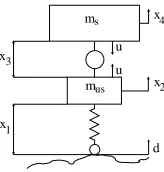
A. Car suspension system modeling

We use the quarter car model as the mathematical descrip-tion of the suspension system, following the model used in [3]. The schematic diagram of the model is shown in Figure 1. In this model, the suspension actuator is taken to be a force actuator acting between the car body (the sprung mass) and the axle of the car. The tire is an ideal, undamped spring between the axle and the ground. Finally, the axle and wheel assemblies are represented as a mass (the unsprung mass) connected to the ground via the tire spring. As shown in Figure 1, the suspension force also reacts against the unsprung mass.

ms

m u

u

d x x

2 4

x₁ x₃

us

Fig. 1. The quarter car suspension model

A linear time invariant dynamic model of the system is represented as follows:

˙

x1=x2−d, x˙3=−x2+x4

˙

x2=−ω2x1+ρu, x˙4=−u

(23)

wherex1 - tire de¤ection (m), x2 - unsprung mass velocity

(m/sec), x3 - suspension de¤ection (m) and x4 - sprung

mass velocity (m/sec). The parameter ω is the unsprung mass natural frequency, ρ is the sprung to unsprung mass ratio and assume that the travel limit of the suspension is

±D. In other words, as long as the suspension de¤ectionx3

satis£es−D < x3< D, the suspension will not bottom out.

Following [3], we use the parameters ω = 2π·10 rad/sec,

ρ:=ms/mus=10,D=0.1 m.

B. Discrete-time backstepping controller design

To obtain a strict feedback form, the state equations are reordered using the following diffeomorphism:

z1=x1+_ρ+1ρ x3, z3=x3

z2=_ρ+11 x2+_ρ+1ρ x4, z4=−x2+x4

The model is then rewritten in the following form

˙

z1=z2−d (24)

˙

z2=− ω

2

ρ+ 1z1+

ρω2

(ρ+ 1)2z3 (25) ˙

z3=z4 (26)

˙

z4=ω2z1−

ρω2

ρ+ 1z3−(1 +ρ)u= ˜u (27)

The Euler model of the system in a strict feedback form is written as follow:

z1(k+ 1) =z1(k) +T(z2(k)−d) (28)

z2(k+ 1) =z2(k) +T(−ω 2_z1(k)

ρ+ 1 +

ρω2_z3(k)

(ρ+ 1)2 ) (29)

z3(k+ 1) =z3(k) +T z4(k) (30)

z4(k+ 1) =z4(k) +T(ω2z1(k)−ρω

2_z3(k)

ρ+ 1

−(1 +ρ)u(k)) =z4(k) +Tu˜(k) (31)

initial conditions. Therefore, the problem is simpli£ed to an asymptotic stabilization problem. We follow similar design steps to those done in [3], applying the Euler based back-stepping design [9] as cited in Subsection 3.2. Due to space limitation, some trivial steps are omitted.

Step 1: From the continuous-time model, it can be seen that

if z3 ≡ 0, then subsystem (28), (29) is marginally stable.

We design a virtual feedback control lawz3d(z1, z2) which

is bounded between −D and D and renders the origin of the closed-loop (z1, z2) subsystem SP-AS. A control that

satis£es this is

z3d=−Dtanh(k1z2

D ), k1>0. (32)

Unfortunately, the candidate Lyapunov function

V0T1(z1, z2) =

1 2

ω2

ρ+ 1z

2 1+

1 2z

2

2 , (33)

which was used in the continuous-time design [3], gives

∆V0T1 ≤ −T M z2tanh(z2) +T ν01 (34)

with z3 = z3d, which is negative semide£nite with small

offsetν01>0.

While we can apply LaSalle Invariance Principle for the continuous-time case, we cannot do the same for the sampled-data design when semiglobal stability condition occurs. The Euler based backstepping [9] we use does not facilitate this condition, and the candidate Lyapunov function

V0T1 does not satisfy the £rst condition of Theorem 3.1. To

200 400 600 800 1000 1200 1400

–40 –20

20 40 z2

–2 –1

1 2

z1

–0.05 –0.04 –0.03 –0.02 –0.01 –1.5

–1 –0.5

0.5 1

1.5 z2

–0.02 –0.01

0.01 0.02

z1

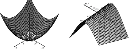
Fig. 2. Surface plots forV0_T1 (l) and∆V0T1 (r), withT= 0.001sec.

solve this problem, we apply Corollary 5.1 of [6] to construct a SP-AS Lyapunov function for subsystem (28), (29). It has been shown earlier that V0T1(z1, z2) is in fact a SP-qISS

Lyapunov function for the subsystem. The surface plots of

V0T1 and∆V0T1 are shown in Figure 2.

To show that the subsystem is SP-AS, we introduce another function

V0T2(z1, z2) =

1 2

ω2

ρ+ 1z

2 1+

1 2z

2 2+ε

z1z2 (1 +z2

1)3/4

. (35)

For small sampling period T > 0 and small ε > 0, the Lyapunov difference of∆V0T2 satis£es

∆V0T2≤ −T M z2tanh(z2)−T M1z

2 1 +T M3(z22+ tanh2(z2)) +T ν02

(36)

with some M, M1, M3 > 0. Hence, V0T2 is a SP-IOSS

Lyapunov function for the £rst two subsystems.

From (34) and (36), it is obvious that the condition (21) is satis£ed, and hence all conditions of Corollary 5.1 of [6] holds. Hence, we can conclude that for some ρ∈ K∞, the functionV0Ta that satis£es

V0Ta=V0T1+ρ(V0T2) (37)

is a SP-AS Lyapunov function for the £rst two subsystems. The surface plots of V0T2 and ∆V0T2 are shown in Figure

3. Suppose we are given a set of initial conditions, such that the SP-AS property of the subsystem (28), (29) is guaranteed withT = 0.001 sec. For a £xε= 0.1, choosing an appropriate ρ ∈ K∞, then we can use formula (37) to combine Figure 2 and Figure 3 after scaling V0T2 with the

functionρ, to show the SP-AS Lyapunov surfaceV0Ta and

the SP-AS difference∆V0Ta of the subsystem (28), (29), for

the given set of initial conditions. Choosing ρ(·) = Id(·)

200 400 600 800 1000 1200 1400

–40 –20

20 40 z2

–2 –1

1 2

z1

–0.0006 –0.0005 –0.0004 –0.0003 –0.0002 –0.0004

0.0002 0.0004

0.0006 0.0008

0.001 z2

–1 –0.8 –0.6 –0.4 0.2 0.4 0.6 0.8 1

z1

Fig. 3. Surface plots forV0_T2 (l) and∆V0T2 (r), withT = 0.001sec

andε= 0.1.

results in a Lyapunov function

V0Ta=V0T1+V0T2 (38)

for the subsystem (28), (29), and we can immediately see that withz3 =z3d the Lyapunov difference ∆V0Ta = ∆V0T1+

∆V0T2 is negative de£nite and hence the subsystem (28),

(29) is SP-AS.

Remark 4.1: We emphasize that choosing ρ= Id in our case is possible since we are dealing with a semiglobal practical property. TheV0Taobtained does not hold globally,

because of the saturation coming from the tanh function inz3d. We also have to choose a small ε to guarantee that ∆V0Ta does not become positive for quite largez2. ¥

To continue the design procedure, for the purpose of simpler computation, we choose to use

V0T =1

2V0Ta =

1

2(V0T1+V0T2), (39)

Step 2: We de£neξ1=z3−z3d(z2)and denoteξ2:= ˙ξ1to

obtain the following third order Euler model:

z1(k+ 1) =z1+T z2

z2(k+ 1) =z2+T

µ

− ω

2

ρ+ 1z1+

ρω2

(ρ+ 1)2(z3d+ξ1)

¶

ξ1(k+ 1) =ξ1+T ξ2 . (40)

Using a candidate Lyapunov function

V1T(z1, z2, ξ1) =V0T(z1, z2) +k2

ξ2

1

2 , k2>0 (41)

and choosing the stabilizing controller as

ξ2d=−1

k2

ρω2

(ρ+ 1)2(z2+

εz1

(1 + (z1+T z2)2)3/4

)−k3ξ1,

withk3>0, we have

∆V1T = ∆V0T|z3d−T k2k3ξ

2

1+T ν1 , (42)

which is negative de£nite with a small offsetν1>0. Hence,

the equilibrium (z1, z2, ξ1) = (0,0,0) is SP-AS. Since

z3d(0) = 0 we can conclude that the origin (z1, z2, z3) = (0,0,0)is also SP-AS.

Step 3: Backsteppingξ2 through an integrator results in the

dynamical system, whose Euler model can then be written as follow:

z1(k+ 1) =z1+T z2

z2(k+ 1) =z2+T(−

ω2

ρ+ 1z1+

ρω2

(ρ+ 1)2(z3d+ξ1))

ξ1(k+ 1) =ξ1+T ξ2 (43)

ξ2(k+ 1) =ξ2+Tu .˜˜

At this step, we consider a candidate Lyapunov function

V2T(z1, z2, ξ1, ξ2) =V1T(z1, z2, ξ1) +k4

2 (ξ2−ξ2d) 2 _,

withk4>0. We apply the formula (17) to obtainu˜˜T using

the following terms:

αT =

−ρω2

k2(ρ+ 1)2(z2+

εz1

(1 + (z1+T z2)2)3/4

)−k3ξ1

WT =

k2

2k4

ξ2

1 ,

(it turns out thatαT :=ξ2d) and get

∆αT

T =

ξ2d(k+ 1)−ξ2d(k)

T

=−1

k2

ρω2

(ρ+ 1)2

µ

ζ2+

εz1

(1 + (z1+ 2T z2+T2ζ2)2)3/4

¶

− 1

k2T

ρω2

(ρ+ 1)2εz1

µ

1

(1 + (z1+ 2T z2+T2ζ2)2)3/4

− 1

(1 + (z1+T z2)2)3/4

¶

−k3z4

− 1

Tk3D(tanh(z2+T ζ2)−tanh(z2)), (44)

whereζ2:=−ω

2

ρ+1z1+ ρω2

(ρ+1)2z3, and

∆WT =V1+T(ξ1+T ξ2)−V1+T(ξ1+T ξ2d)

= k2 2k4

(2T ξ1ξ2−2T ξ1ξ2d+T2ξ22−T2ξ22d).

Moreover, using (19) we have

g

∆WT

T =

k2

k4

ξ1+

k2T

2k4

(ξ2+ξ2d). (45)

Hence, we obtainu˜˜= ˜˜uT by substituting (44),(45) to

˜˜

uT =−

k5

k4

(ξ2−ξ2d)−

g

∆WT

T +

∆αT

T , k5>0. (46)

It can be shown that implementingu˜˜T to the system results in ∆V2T negative de£nite with small offsetν2>0. This means

that the equilibrium (z1, z2, ξ1, ξ2) = (0,0,0,0) is SP-AS.

Sincez3d(0) = 0, then the origin(z1, z2, z3, z4) = (0,0,0,0)

is also SP-AS.

We have seen earlier thatV1T satis£es the SP-ISS (in this

case SP-AS) Lyapunov condition of Theorem 3.1. It is then obvious that withV2T that the £rst condition of Theorem

3.1 still holds.

Step 4: Following exactly as in the continuous-time design,

the resulting control lawu=uT that SPA stabilizes the Euler

model (28)-(31) has form

uT =

1

ρ+ 1(−u˜˜T−∆ζ3d+ω

2_{x1) (47)}

with ∆ζ3d := ¨z3d. Finally, by substituting the appropriate

terms, we haveuT as a nonlinear control law parameterized

by the sampling periodT and £ve positive tuning parameters

k1, k2, k3, k4 andk5.

ExpandinguT in series representation, we can show that

uT satis£es the third condition of Theorem 3.1. Since all

conditions of Theorem 3.1 hold, we can guarantee that uT

SPA stabilizes the closed-loop approximate model, and also stabilize the closed-loop exact model. We further use results from [8], to conclude the SP-AS for the sampled data system (23), (47).

C. Comparing the Euler-based controller with the Emula-tion controller

We have designed a discrete-time backstepping controller (47) that SPA stabilizes the active suspension system. Now, we implement the controller (47), and observe the perfor-mance of the closed-loop sampled-data system with the designed controller, and compare it with a controller that has form:

u= 1

ρ+ 1(−u˜˜−∆ζ3d+ω

2_{x1) (48)}

whereu˜˜= ∆ξ2d−k_k2₄ξ1 −k_k5₄(ξ2−ξ2d),with∆ξ2d:= ˙ξ2d.

period (using zero order hold). By applying Corollary 5.1 of [5], we can show that the discrete-time emulation controller (48) also SPA stabilizes the continuous-time plant (23).

We study the condition when there are small offsets to the initial states, in other words, when allowing nonzero initial states. We observe the responses of the system to bumps of different heights and compare the performance of each controller. The shape of the isolated bump 1 _{is chosen to be}

in the form that gives rise to the following velocity input:

d(t) =

    

0, t≤0

10πAsin(20πt), 0< t≤0.1

0, t >0.1.

(49)

We £rst run the Simulation Road-1 (see Figure 4), when setting T = 0.001 sec, initial states (0.01 0 0.01 0)T _and

bump heightA= 0.01m.

0 0.1 0.2 0.3 0.4

−5 0 5 10

15x 10

−3 _(a)

x1

0 0.1 0.2 0.3 0.4

−1.5 −1 −0.5 0 0.5

(b)

x4

−x

2

0 0.1 0.2 0.3 0.4

−2 0 2 4 6 8 10

12x 10

−3 (c)

t (sec)

x3

0 0.01 0.02 0.03 0.04

−50 0 50 100 150

t (sec)

u

(d)

Fig. 4. Simulation Road-1 for a low bump condition,· · · emulation and

Euler.

In Simulation Road-2 (see Figure 5), we set A = 0.1

meter, which is considered as a high bump. We setT = 0.001

sec and initial states(0.01 0 0.01 0)T_.

From the two sets of simulation, we see that the system can always achieve better performance with the Euler based controller than with the emulation controller.

V. REFERENCES

[1] J.P. Barbot and S. Monaco and D. Normand-Cyrot, A sampled normal form for feedback linearization, Math.

Contr. Sig. Sys., vol. 9, 1996, pp 162-188.

[2] F. Esfandiari and H.K. Khalil, On the robustness of sampled-data control to unmodelled high frequency dynamics, IEEE TAC, vol. 34, 1989, pp 900-903. [3] N. Karlsson, A. Teel and D. Hrovat, ”A backstepping

approach to control of active suspensions”, Proc. IEEE

CDC, Orlando, FL, 2001, pp 4170-4175.

1_{this kind of bump is a haversine of heightAm and length l= 2 m,}

while assuming the vehicle is traversing the road at a speed ofv= 20m/s.

0 0.1 0.2 0.3 0.4

−0.06 −0.04 −0.02 0 0.02 0.04 0.06

(a)

x1

0 0.1 0.2 0.3 0.4

−2 −1 0 1 2

(b)

x4

−x

2

0 0.1 0.2 0.3 0.4

−0.06 −0.04 −0.02 0 0.02

0.04 (c)

t (sec)

x3

0 0.01 0.02 0.03 0.04

−50 0 50 100

150 (d)

t (sec)

u

Fig. 5. Simulation Road-2 for a high bump condition,· · · emulation and

Euler.

[4] M. Krsti´c, I. Kanellakopoulos and P. V. Kokotovi´c,

Nonlinear and Adaptive Control Design, Wiley; 1995.

[5] D.S. Laila, D. Ne³si´c and A.R. Teel, Open and closed loop dissipation inequalities under sampling and con-troller emulation, European Journal of Control, vol. 8, 2002, pp 109-125.

[6] D.S. Laila and D. Ne³si´c, Changing supply rates for input-output to state stable discrete-time nonlinear sys-tems with applications, Automatica, vol. 39, 2003, pp 821-835.

[7] D. Ne³si´c and D.S. Laila, A note on input to state stabilization for nonlinear sampled-data systems, IEEE

TAC., vol. 47, 2002, 1153-1158.

[8] D. Ne³si´c A.R. Teel and E.D. Sontag, Formulas relating

KL stability estimates of discrete-time and sampled-data nonlinear systems, SCL, vol. 38, 1999, pp 49-60. [9] D. Ne³si´c and A.R. Teel, ”Backstepping on the Euler

approximate model for stabilization of sampled-data nonlinear systems”, Proc. IEEE CDC, Orlando, FL, 2001, pp 1737-1742.