Pseudo-Boolean Optimization
Vasco M. Manquinho and Jo˜ao Marques-Silva
IST/UTL, INESC-ID, Portugal, [email protected], [email protected]
Abstract. Linear Pseudo-Boolean constraints offer a much more compact formalism to express significant boolean problems in several areas, ranging from Artificial Intelligence to Electronic Design Automation. This paper proposes a new algorithm for the Pseudo-Boolean Optimization Problem (PBO) which integrates features from recent advances in Boolean Satisfiability (SAT) and classical branch and bound algorithms. Moreover, the paper shows that the utilization of lower bound estimates can improve the overall performance of PBO solvers for different classes of instances. In addition, the paper describes how to apply non-chronological backtracking in the presence of conflicts that result from the bounding process. Finally, the paper also shows how the notion of Unique Implication Points (UIP), widely used in modern SAT solvers, can be generalized for PBO.
1
Introduction
In [2], P. Barth first proposed a SAT-based approach for solving pseudo-boolean optimization. This approach consists of performing a linear search on the possible values of the cost function, starting from the highest, at each step requiring the next computed solution to have a cost lower than the previous one. If the resulting instance is not satisfiable, then the solution is given by the last recorded solution. Along with recent advances in SAT solvers, new pseudo-boolean solvers and optimizers emerged using the same approach but with better results. The incorporation in solvers of non-chronological backtracking in the search tree, conflict-based learning mechanisms and lazy data structures have proved to be effective in solving pseudo-boolean instances [1, 4, 7].
In this paper we start by describing how a classical lower bound estimation method from the covering domain can be adapted for a pseudo-boolean optimization algorithm. In section 3 we focus on how to obtain explanations on bound-conflict situations that allow backtracking non-chronologically when the search is bound due to the lower bound estimation and we also describe how to reduce those explanations. In section 5 we present a generalization of the notion ofunique implication points(UIP) to strengthen the learning process in pseudo-boolean formulations. Finally, we present some experimental results and the paper concludes in section 7.
2
Preliminaries
In a propositional formula, a literallj denotes either a variablexj or its complement ¯xj. If a literal
lj =xj andxj is assigned value 1 orlj = ¯xj andxj is assigned value 0, then the literal is said to be true. Otherwise, the literal is said to be false.
An instanceP of a Linear Pseudo-Boolean Optimization problem can be defined as follows,
minimize n
P
j=1
cj·xj
subject to n
P
j=1
aijlj ≥bi,
xj∈ {0,1}, aij, bi∈N +
0 , i∈ {1..m}
(1)
In a given constraint, if allaij coefficients have the same valuek, then it is called a cardinality constraint, since it only requires that ⌈bi/k⌉literals be true. A pseudo-boolean constraint where any literal set to true is enough to satisfy the constraint, can be interpreted as a propositional clause. This occurs when the value of allaij coefficients are greater than or equal to bi.
If every constraint can be interpreted as a propositional clause then C is an instance of the binate covering problem(BCP). Covering formulations have been the subject of thorough research work that can be found in [5, 10, 14].
3
Estimation of Lower Bounds
The most widely used approach for solving pseudo-boolean problems is the classical branch-and-bound procedure [6, 9] in which upper boundson the value of the cost function are identified for each solution to the constraints, andlower boundson the value of the cost function are estimated considering the current set of variable assignments. The search is pruned whenever the lower bound estimate is higher than or equal to the upper bound. In these cases we can guarantee that a better solution cannot be found with the current variable assignments and therefore the search can be pruned. The algorithms described in [5, 9, 14] for the binate covering problem follow this approach as well as several general integer programming solvers.
Branch and bound algorithms are proved to be very effective when the instances to be solved are not highly constrained [5, 9]. With those instances, the tightness of the lower bounding procedure is crucial for the algorithm’s efficiency, because with higher estimates of the lower bound, the search can be pruned earlier. For binate covering, the most commonly used lower bound estimation procedure is the approximation of a maximum independent set of clauses [6]. However, other procedures can be used, namely the ones based on linear-programming relaxations [9]. Given a lower bound value, additional techniques can be applied, namely the limit lower bound, first proposed in [6], that we describe in this section.
3.1 Maximum Independent Set
The maximum independent set of constraints (MIS) is a greedy method to estimate a lower bound on the value of the cost function based on an independent set of constraints. A more detailed definition applied to binate covering can be found in [6]. Here we describe its generalization to pseudo-boolean problems.
The greedy procedure consists of finding a set MISof disjoint constraints (i.e. with no costly literals in common among them), with a minimum cost to be satisfied greater than zero. Since maximizing the cost of MIS is an NP-hard problem, a greedy computation is used. The effec-tiveness of this method largely depends on the constraints included in MIS. Usually, one chooses the constraint which maximizes the ratio between its weight and its number of unassigned costly literals.
In order to build a maximum independent set of constraints, we must determine the minimum cost to satisfy each constraint independently. Remember that a pseudo-boolean constraintωi can be viewed as:
ωi= n
X
j=1
aijlj≥bi, (2)
Suppose all no-cost literals fromωi are true and let snc be the sum of the coefficients of all no-cost literals fromωi, we would have:
ωi′ = n
X
j=1
aijxj≥bi−snc, (3)
Finding the minimum cost for satisfyingω′
i provides the minimum cost to satisfyωi and that can be defined as:
minimize n
P
j=1
cj·xj
subject to ωi′
Since it would not be feasible to solve a pseudo-boolean optimization problem for each con-straint, we define an approximation algorithm for the minimum cost of satisfying a pseudo-boolean constraint. First, we determine the minimum number of literals that need to be true in order to satisfyω′
i by reducingω
′
i to a cardinality constraint [3]. This can be done by summing the sorted set ofωi′ coefficients, starting from the largestaij and checking if the sum of P
n
j=1aij < bi−snc holds for each value ofn. More detailed description of the cardinality reduction algorithm can be found in [4].
Suppose thatωic′ denotes the cardinality constraint obtained by the cardinality reduction algo-rithm applied to ω′i
ω′ic= n
X
j=1
xj≥k, (5)
a lower bound on the minimum cost to satisfy ωi′ is given by accumulating the cost of the firstk literals in a sorted set of literal coefficients in the problem cost function, starting with the lowest
cj.
Building the maximum independent set of constraintsMISis done by, at each step, adding a new constraint with no literal in common with any other constraint already inMIS. The minimum cost for satisfying MISis a lower boundon the solution of the problem instance and is given by,
Cost(M IS) = X ωi∈M IS
M inCost(ωi) (6)
where M inCost(ωi) denotes the lower bound on the minimum cost to satisfy ωi given by the approximation algorithm described in this section.
Although the lower bound provided by the maximum independent set of constraints can be arbitrarily far from the optimum, it is a simple and fast method to determine a lower bound on the problem instance. Linear-programming relaxations [9] usually find much closer bounds, but are much more time consuming, in particular on highly constrained instances.
4
Bound-Based Pruning Techniques
When using lower bound estimations on the value of the cost function, it is possible to apply several techniques that prune the search tree. In this section we explain how to backtrack non-chronologically when using lower bound estimations and also how to prune the search tree based on the estimation value of the cost function.
4.1 Backtracking on Bound-based Conflicts
A bound conflict in an instance of the pseudo-boolean optimization problem (PBO)Parises when the lower bound is equal to or higher than the upper bound. This condition can be written as
P.path+P.lower≥P.upper, whereP.pathis the cost of the assignments already made,P.loweris a lower bound estimate on the cost of satisfying the clauses not yet satisfied (as given for example by an independent set of constraints), and P.upper is the best solution found so far. From the previous equation, we can readily conclude that P.path and P.lower are the unique components involved in each bound conflict. Therefore, we will analyze both P.pathand P.lower components in order to establish the assignments responsible for a given bound conflict.
We start by studyingP.path. Clearly, the variable assignments that cause the value ofP.path to grow are solely those assignments with a value of 1. Hence, we can define a set of literalsωcp, such that each variable in ωcphas positive cost and is assigned value 1:
ωcp={l= ¯xj :Cost(xj)>0∧xj = 1} (7)
which basically states that to decrease the value of the cost function (i.e. P.path) at least one variable that is assigned value 1 has instead to be assigned value 0.
in M IS is part of M IS because it is neither satisfied nor has common literals with any other constraint in M IS. Clearly, for each constraint ωi ∈M IS these conditions only hold due to the literals in ωi that are assigned value 0. If any of these literals was assigned value 1,ωi could be satisfied. Consequently, we can define a set of literals that explain the value of P.lower:
ωcl={l:l= 0∧l∈ωi∧ωi∈M IS} (8)
Now, as stated above, a bound conflict is solely due to the two components P.pathand P.lower. Hence, this bound conflict will hold as long as the following clauseωbc is unsatisfied:
ωbc=ωcp∪ωcl (9)
(Observe that the set union symbol in the previous equation denotes a disjunction of literals.) As long as this clause is unsatisfied, the values ofP.pathand P.lowerwill remain unchanged, and so the bound conflict will exist. We can thus use this unsatisfied clause ωbc to analyze the bound conflict and decide where to backtrack to, using a conflict analysis procedure. We should observe that backtracking can be non-chronological, because clauseωbcdoes not necessarily depend on all decision assignments. Moreover, due to the clause recording mechanism, ωbc can be used later in the search process to prune the search tree.
4.2 Reducing Bound Dependencies
After a careful analysis on how the bound explanation clause is built, several techniques can be devised in order to reduce the number of dependencies when a bound conflict occurs.
For instance, suppose that we havexj = 1 and that a bound conflict arises. According to (7), ¯
xj would be inωcp. However, if we find a constraintωithat is satisfied due toxj = 1 and if setting or changing the value of any other literal inωiwould satisfy the constraint with a cost higher than or equal to the cost of setting xj to 1, then the value xj is irrelevant for the bound conflict to arise. Note that even in pseudo-boolean optimizers that do not use lower bound estimations, this technique can be used to reduce the number of dependencies when a new solution is found.
A similar approach can be used to reduce the number of dependencies in ωcl. Suppose that there is a literal xj ∈ωcl because xj = 0 andxj is a literal in a single constraint ωi ∈M IS. If settingxjto 1 is more costly than any other set of assignments to satisfyωi, thenxj is not relevant to explain the bound conflict.
4.3 Limit Lower Bound Theorem
The limit lower bound was first proposed in [6]. It states that by using lower bound estimation methods, one can also prune the search tree by identifying some necessary assignments. That occurs whenever after calculating the lower bound estimation we have:
P.path+P.lower+Cost(xj)≥P.upper (10)
when xj is not an unassigned literal in any constraint ωi ∈ M IS, then xj = 0 is a necessary assignment since otherwise a bound conflict would occur.
5
Conflict Analysis Techniques
5.1 Learning Clause Constraints
An implication graph is a directed acyclic graph where each vertex represents a variable assignment and edges represent the reasons that lead to the assignments. A conflict arises when a variable is assigned both value 0 and value 1. In fig. 1 an example of an implication graph is shown where the conflict occurs due to the assignment of 0 and 1 to variable x5. Unique implication points (UIP) in the implication graph are vertexes that represent assignments which by itself are single reasons for the conflict to occur. In fig. 1 assignments tox3andx4 are UIPs.
In pseudo-boolean formulas from a single constraint it is possible to imply several variable assignments. For instance, suppose we have the following constraints:
ω1: 2x1+x2+ 2x3+x4≥3
ω2: 2¯x3+ 3x5≥2
ω3: 3¯x4+ 4¯x5≥3
(11)
where x1 = x2 = 0. In this situation we must necessarily have x3 = x4 = 1 in order to satisfy constraintω1. The implication graph is shown at fig. 2 where we can identify a conflict on variable
x5.
Applying the conflict analysis procedure from [1, 17] we would learn a new clause (x1+x2) that would allow the search to backtrack and change the value of the last decision assignment. However, one should note that there is one cut in the implication graph that only crosses edges from constraint ω1. We can interpret this situation as an UIP at the edge level instead of at a vertex. Therefore, we can add a new clause representing a cut in the graph that only intercepts antecedent edges from a single constraint. In this case we would add a clause (¯x3+ ¯x4).
Notice that clauses generated through these graph cuts are not unit when the current decision level is undone. The purpose is to strengthen the set of learned no-goods. Therefore, another new clause must be added according to the procedure described in [17].
6
Experimental Results
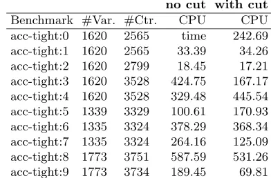
In this section we compare the different algorithmic strategies presented in the paper using our pseudo-boolean solver and optimizer. Our solver was run with a variant of the VSIDS [11] heuristic adapted to deal with pseudo-boolean constraints and keeping all constraints learned during conflict analysis. Neither restarts nor random backtracking were used. The CPU times presented are from a Pentium IV processor at 1.7GHz with 1GB of physical memory. The time limit for each instance was set to one hour.
.
no cut with cut Benchmark #Var. #Ctr. CPU CPU acc-tight:0 1620 2565 time 242.69 acc-tight:1 1620 2565 33.39 34.26 acc-tight:2 1620 2799 18.45 17.21 acc-tight:3 1620 3528 424.75 167.17 acc-tight:4 1620 3528 329.48 445.54 acc-tight:5 1339 3329 100.61 170.93 acc-tight:6 1335 3324 378.29 368.34 acc-tight:7 1335 3324 264.16 125.09 acc-tight:8 1773 3751 587.59 531.26 acc-tight:9 1773 3734 189.45 69.81 Table 1.Results for pseudo-boolean solving
.
no bounds with bounds no bounds with bounds
Benchmark Sol CPU Sol CPU Benchmark Sol CPU Sol CPU
aim-100-1 6-yes1-1 43 0 43 0.01 ii8a1 54 0.27 54 0.05 aim-100-6 0-yes1-3 49 0.03 49 0.04 ii8a2 – time 137 1117.6 aim-200-1 6-yes1-2 105 0.03 105 0.03 ii8a3 – time – time aim-200-3 4-yes1-3 111 0.26 111 0.36 par16-1-c 107 100.07 107 139.35 aim-50-2 0-yes1-4 26 0 26 0.01 par16-2 300 165.51 300 215.29 aim-50-3 4-yes1-2 28 0.01 28 0.01 par8-1-c 26 0 26 0.02
jnh17 67 0.08 67 0.09 par8-2 64 0.04 64 0.04
jnh1 55 0.48 55 0.94 par8-5-c 37 0.01 37 0.01
jnh201 62 111.08 62 8.19 qg1-07 49 8.83 49 7.69
jnh213 66 0.05 66 0.09 qg2-07 49 8.79 49 7.91
jnh217 69 8.22 69 4.98 qg3-08 64 16.64 64 29.87
[image:6.612.206.402.79.208.2]jnh218 67 0.1 67 0.13 qg7-09 81 0.85 81 1.41
Table 2.Results for pseudo-boolean optimization
are in general improvements in CPU time in finding solutions for this benchmark set. When the solver was unable to find the solution, the reason is presented.
In the experiment with our optimization algorithm we tested it by generating instances of the Max-ONE problem (using a minimization model) from several instances of the DIMACS [8] and quasi-group [16] benchmarks set. In table 2 we present the results from our algorithm when using and not using lower bound estimates. Notice that in some instances, the algorithm is able to prune the search tree due to the lower bound estimates and therefore is able to faster prove optimality of the solution found. However, when the instance is harder to satisfy, few bound conflicts are observed and the lower bounding mechanism mostly adds an overhead to the algorithm.
7
Conclusions
This paper describes the generalization of the maximum independent set of constraints as a lower bound mechanism to the linear pseudo-boolean optimization problem. In the paper we also present conditions that allow for non-chronological backtracking in the presence of bound conflicts. More-over, preliminary results show that in some instances where the lower bound procedure is effective, search can be pruned and improve the performance of pseudo-boolean solvers. In the paper we also describe how to generalize the notion of Unique Implication Points to the linear pseudo-boolean optimization.
8
Acknowledgements
This work is partially supported by the European research project IST-2001-34607 and by Funda¸c˜ao para a Ciˆencia e Tecnologia under research projects POSI/CHS/34504/2000 and POSI/SRI/-41926/2001.
References
1. F. Aloul, A. Ramani, I. Markov, and K. Sakallah. PBS: A Backtrack-Search Pseudo-Boolean Solver. In
Symposium on the Theory and Applications of Satisfiability Testing (SAT), pages pp. 346–353, 2002. 2. P. Barth. A Davis-Putnam Enumeration Algorithm for Linear Pseudo-Boolean Optimization. Technical
Report MPI-I-95-2-003, Max Plank Institute for Computer Science, 1995.
3. P. Barth. Logic-Based 0-1 Constraint Programming. In . Kluwer Academic Publishers, 1995. 4. D. Chai and A. Kuehlmann. A Fast Pseudo-Boolean Constraint Solver. InDesign Automation
Con-ference, 2003.
5. O. Coudert. On Solving Covering Problems. In Proceedings of the ACM/IEEE Design Automation Conference, pages 197–202, June 1996.
6. O. Coudert and J. C. Madre. New Ideas for Solving Covering Problems. In Proceedings of the
ACM/IEEE Design Automation Conference, June 1995.
7. H. Dixon and M. Ginsberg. Inference Methods for a Pseudo-Boolean Satisfiability Solver. InNational Conference on Artificial Intelligence, 2002.
8. D. S. Johnson and M. A. Trick, editors. Second DIMACS Implementation Challenge. American Mathematical Society, 1993.
9. S. Liao and S. Devadas. Solving Covering Problems Using LPR-Based Lower Bounds. InProceedings
of the ACM/IEEE Design Automation Conference, pages 117–120, 1997.
10. V. Manquinho and J. Marques-Silva. Search pruning techniques in sat-based branch-and-bound algo-rithms for the binate covering problem. IEEE Transactions on Computer-Aided Design, 2002. 11. M. Moskewicz, C. Madigan, Y. Zhao, L. Zhang, and S. Malik. Chaff: Engineering an Efficient SAT
Solver. InDesign Automation Conference, June 2001.
12. M. Savelsbergh. Preprocessing and probing for mixed integer programming problems. ORSA Journal
on Computing, 6:445–454, 1994.
13. J. P. M. Silva and K. A. Sakallah. GRASP-A search algorithm for propositional satisfiability. IEEE
Transactions on Computers, 48(5):506–521, May 1999.
14. T. Villa, T. Kam, R. K. Brayton, and A. L. Sangiovanni-Vincentelli. Explicit and Implicit Algorithms for Binate Covering Problems. IEEE Transactions on Computer Aided Design, vol. 16(7):677–691, July 1997.
15. J. Walser. 0-1 integer programming benchmarks. http://www.ps.uni-sb.de/∼ walser/benchmarks/-benchmarks.html.
16. H. Zhang. SATO: An efficient propositional prover. InProceedings of the International Conference on
Automated Deduction, pages 272–275, July 1997.