Retrieval of suspended sediment concentration in near shore coastal waters using MODIS data : a thesis presented in partial fulfilment of the requirements for the degree of Master of Philosophy in Earth Science at Massey University, Palmerston North, New

Full text

(1)Copyright is owned by the Author of the thesis. Permission is given for a copy to be downloaded by an individual for the purpose of research and private study only. The thesis may not be reproduced elsewhere without the permission of the Author..

(2) Retrieval of suspended sediment concentration in near-shore coastal waters using MODIS data. A thesis presented in partial fulfilment of the requirements for the degree of Master of Philosophy In Earth Science At Massey University, Palmerston North New Zealand. Di Zhou 2012. 1.

(3) Abstract:. This study focuses on using remote sensing satellite data to retrieve water suspended sediment concentration (SSC) of near-shore coastal waters. Aqua/Terra Satellite MODIS 250m data of the south-western coast of the North Island, New Zealand was used. Two methods of analysis are used in this study to obtain an SSC map; non-liner optimisation and quasi-analytical.. The non-linear optimisation method was used to fit an exponential function between reflectance and SSC, with SSC replaced by a linear relationship between SSC and reflectance in the near infrared domain. The optimisation result was used to convert Aqua/Terra MODIS images to SSC maps.. The quasi-analytical method, a backscattering coefficient at 645nm is first derived from Aqua/Terra MODIS 250m Band 1 data using a quasi-analytical algorithm after applying a simple atmospheric correction routine. An empirical relationship was derived from laboratory experiments. Finally SSC maps were obtained by applying the empirical relationship to convert the backscattering coefficient to SSC.. 2.

(4) Acknowledgements. I would firstly like to thank my supervisor Mike Tuohy for his time and thoughtful advice throughout the preparation of this thesis. I would also like to thank Horizons Regional Council for providing the daily mean flow and sediment load (flow) data of the research area.. 3.

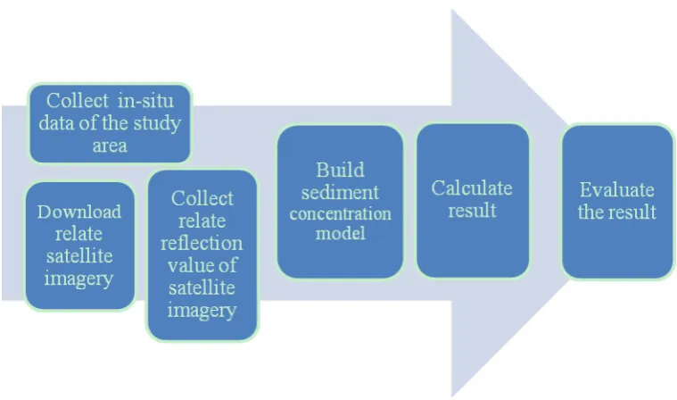
(5) Table of Contents. 1 Introduction .................................................................................................................... 1 1.1 Atmospheric Correction .......................................................................................... 5 1.2 Remote Sensing Satellite......................................................................................... 6 1.2.1 Terra Satellite ................................................................................................... 6 1.2.2 Aqua Satellite ................................................................................................... 7 1.3 MODIS .................................................................................................................... 8 1.4 Literature Review .................................................................................................... 9 1.4.1 Empirical Approach........................................................................................ 10 1.4.2 Analytical Approach ....................................................................................... 12 1.4.3 Non-linear Optimisation Approach ................................................................ 16 1.5 Rivers .................................................................................................................... 17 1.6 Horizons Regional Council ................................................................................... 18 2 Method ......................................................................................................................... 19 2.1 Study Area ............................................................................................................. 19 2.2 Data Download ...................................................................................................... 19 2.3 Georeferencing and Bow Tie Effect Correction ................................................... 21 2.4 Atmospheric Correction ........................................................................................ 22 2.5 SSC Retrieve ......................................................................................................... 23 2.5.1 Non-linear Optimisation ................................................................................. 23 2.5.2 Quasi-analytical .............................................................................................. 27 2.6 Laboratory Experiments ........................................................................................ 33 2.6.1 Instruments: .................................................................................................... 33 2.6.2 Instruments Set Up ......................................................................................... 34 2.6.3 Spectral Measurements ................................................................................... 35 3 Results and Discussion: ............................................................................................... 36 3.1 Laboratory Experiments ........................................................................................ 36 3.2 SSC Retrieval ........................................................................................................ 44 3.2.1 SSC Map ......................................................................................................... 45 3.2.2 Total Sediment Calculation ............................................................................ 59 4 Conclusion and future work ......................................................................................... 66 5 References .................................................................................................................... 67 4.

(6) List of Tables. Table 1.1 SSC retrieval methods………………………………………………………...4 Table 1.3.1 MODIS Band 1 & 2…….....………………………………………………...9 Table 2.5.2.1 Relationship between the backscattering coefficient and SSC…...…..…30 Table 3.2.1.1 Daily mean flow data (l/s) of four river monitoring stations …………...45 Table 3.2.1.2 Sediment Load (Kg/m3) of four river monitoring stations……………...45 Table 3.2.1.3 Daily mean flow data (l/s) of four river monitoring stations……………46 Table 3.2.1.4 Sediment Load (Kg/m3) of four river monitoring stations……………...46 Table 3.2.1.5 Daily mean flow data (l/s) of four river monitoring stations……………48 Table 3.2.1.6 Sediment Load (Kg/m3) of four river monitoring stations……………...48 Table 3.2.1.7 Daily mean flow data (l/s) of four river monitoring stations……………49 Table 3.2.1.8 Sediment Load (Kg/m3) of four river monitoring stations……………...49 Table 3.2.1.9 Daily mean flow data (l/s) of four river monitoring stations……………52 Table 3.2.1.10 Sediment Load (Kg/m3) of four river monitoring stations…………….52 Table 3.2.1.11 Daily mean flow data (l/s) of four river monitoring stations…………..54 Table 3.2.1.12 Sediment Load (Kg/m3) of four river monitoring stations…………….54 Table 3.2.1.13 Daily mean flow data (l/s) of four river monitoring stations…………..55 Table 3.2.1.14 Sediment Load (Kg/m3) of four river monitoring stations…………….55 Table 3.2.1.15 Daily mean flow data (l/s) of four river monitoring stations…………..56 Table 3.2.1.16 Sediment Load (Kg/m3) of four river monitoring stations…………….56 Table 3.2.1.17 Daily mean flow data (l/s) of four river monitoring stations…………..57 Table 3.2.1.18 Sediment Load (Kg/m3) of four river monitoring stations…………….57 Table 3.2.2.1 High suspended sediment area 11 April 2011………………..…………62 Table 3.2.2.2 High suspended sediment area 24 January 2011………………………..64 Table 3.2.2.3 High suspended sediment area 29 April 2011………………………..…65 5.

(7) List of Figures. Figure 1.4.1 General SSC retrieving scheme………………………………….………..10 Figure 1.4.1.1 Location map of the three study areas (Lake Pontchartrain, Mississippi River Delta, and Mississippi Sound) in the northern Gulf of Mexico…………………...……11 Figure 1.4.1.2 Empirical relation between total suspended matter (TSM) and reflectance of Terra MODIS 250m band 1 (O) Mississippi Sound 16 May 2001; (●) Mississippi River Delta 17 March 2002; (□)Mississippi River Delta 15 July 2003; (■) Lake Pontchartrain 19 May 2002; (Δ) Lake Pontchartrain 23 May 2002; (▲)Mississippi River Delta 20 October 2003……………………………………………………………………………………..12 Figure 1.4.2.1 The average SIOP of Teluk Banten ………………………………….…14 Figure 1.4.2.2 (a) Algorithm based on SPOT HRV; (b) algorithm based on LandSat TM5……………………………………………………………………………….…….15 Figure 1.4.3.1: Comparison of simulated and in-situ measurements of suspended sediment concentrations…………………………………………………………………………..16 Figure 1.6.1 Four river monitoring stations……………………………………….……18 Figure 2.1.1 Satellite image of South West coast of North Island, New Zealand ….….19 Figure 2.2.1 LAADS Product Selection………………………………………….…….20 Figure 2.2.2 Select download region…………………………………………….……..21 Figure 2.3.1 Georeferencing and bow tie effect correction……………………….……22 Figure 2.4.1 FLAASH Atmospheric Correction Model Input Parameters………….….23 Figure 2.5.1.1 Optimizing Excel worksheet.…………………….……………………..26 Figure 2.5.2.1 Absorption coefficient variations at different wavelengths………….…29 Figure 2.2.2.2 Empirical relation between backscattering coefficient and SSC……….31 Figure 2.6.2.1 Instruments set up………………………………………………………35 Figure 3.1.1 Reflectance spectra of different papers…………………………………..36 Figure 3.1.2 Reflectance spectra of different containers on black background………..37 Figure 3.1.3 Reflectance spectra of different depths of pure water (white container on the black background)…………………………………………………………………..….38. 6.

(8) Figure 3.1.4 Reflectance spectra of different depths of salt water (30g/l) (white container on the black background)…………………………………………………….………..….39 Figure 3.1.5 Reflectance spectra of different depths of salt water (30g/l) (white container on the white background)…………………………………………………………………40 Figure 3.1.6 Reflectance spectra of different light angle (pure water 20cm water height, white container on the white background)………………………………………….………..41 Figure 3.1.7 Reflectance spectra of different light angle (pure water 15cm height, white container on the white background)……………………………………………………42 Figure 3.1.8 Reflectance spectra of different SSC (salt water 20cm height, white container on the black background)…………………………………………………………….……43 Figure 3.2.1.1 Terra 18 January………………………………………………………...45 Figure 3.2.1.2 Aqua 19 January………………………………………………………...46 Figure 3.2.1.3 Terra 24 January………………………………………………………...48 Figure 3.2.1.5 Daily mean flow ………………………………………………………..50 Figure 3.2.1.6 Sediment Load………………………………………………………….50 Figure 3.2.1.7 Terra 28 January………………………………………………………...51 Figure 3.2.1.8 Daily mean flow………………………………………………………...53 Figure 3.2.1.9 Sediment Load………………………………………………………….53 Figure 3.2.1.10 Terra 11 April………………………………………………………….54 Figure 3.2.1.11 Aqua 12 April…………………………………………………………55 Figure 3.2.1.12 Terra 28 April………………………………………….………………56 Figure 3.2.1.13 Aqua 29 April………………………………………………………….57 Figure 3.2.2.1 From contour maps to DEM…………………………………………....59 Figure 3.2.2.2 Contour maps (a) Wanganui river mouth; (b) Whangaehu river mouth; (c) Rangitikei river mouth; (d) Manawatu river mouth……………………….…………...60 Figure 3.2.2.3 TIN of the study area……………………………………………………60 Figure 3.2.2.4 DEM of the study area…………………………………………..……...61 Figure 3.2.2.5 Near-shore high SSC area (within the red line) 11 April 2011…….......62 Figure 3.2.2.6 Near-shore high SSC area (within the red line) 24 January 2011…….. 64 7.

(9) Figure 3.2.2.7 Near-shore high SSC area (within the red line) 29 April 2011…….....65. 8.

(10) 1 Introduction. Coastal waters are often characterized by high suspended sediment concentration (SSC), especially after floods. This is because by introduction of particulate and dissolved matter to coastal area rivers which discharge into the ocean have a major effect on SSC. Since coastal area SSC is a key indicator of biomass primary production, erosion and deposition processes, transport of nutrients and micro-pollutants, the mapping of the distribution of SSC in coastal waters on a regular basis is important to many scientific and environmental studies.. Currently SSC of near-shore coastal waters are often poorly monitored. This is because traditional ship based surveys are often unable to identify temporal fluctuations and are limited in their ability to monitor the full extent of coastal zone. Such problems may be addressed by using remote sensing technology. Satellite images provide synoptic and frequent overviews of coastal areas enabling a more effective analysis of the temporal and spatial dynamics of turbid near-shore coastal waters. Nowadays there is a wealth of research which discusses the utility of using remote sensing in the monitoring of SSC (Table 1.1).. 1.

(11) Formula. Imagery (location time). Sediment concentration range. Paper. Southern Bohai Strait. 0-500 mg/l. [Bi et al., 2011]. y = 2.7969R646– 1.13792 R=0.94. Mahanadi Estuary, East Coast of India. 1-80 mg/l. [Mishra, 2004]. y = 0.0053x +0.0033 R2=0.5827 (y: 620-670 nm). Pakri Bay (southern part of Gulf of Finland). 3 -11 mg/l. [Sipelgas et al., 2006]. Yangtze River. 50-600mg/l. [Wang and Lu, 2010]. Middle and Lower Yangtze River. 10-900 mg/l. [Wang et al., 2010]. 0-50 mg/l. [Miller and McKee, 2004]. y=44.937x; R2=0.9477 (x: backscatter). Northern Gulf of Mexico (Lake Pontchartrain Mississippi River Delta and Mississippi Sound ) Coastal area of north Singapore. 0 – 36 (NTU). [Liew et al., 2009]. y=exp(2.15×(R645/R555)) ×0.95 R2=0.88. Southern Bohai Strait. 0-500 mg/l. [Bi et al., 2011]. y= 12.996 × exp [(R1/R2)/0.189] R2=0.89 (MODIS Aqua R1:band1 R2: band2). Gironde Estuary. 0-2500 mg/l. [Doxaran et al., 2009]. y= 27.424 × exp [0.0279 (R1/R2)] R2=0.89 (SPOT HRV R1: XS3 R2: XS1). Gironde Estuary. 0-2500 mg/l. [Doxaran et al., 2003]. y = 203.74×(R645/R555) – 270.80. y = 0.262 (B2-B5) + 4.117 (MODIS) y = 60.24 (B2-B5) – 23.03 R2=0.73 (MODIS) y = -1.91 ×1140.25 R2=0.5827 (MODIS band1). R=0.65. R2=0.78. 2.

(12) y= 29.022 × exp [0.0335 (R1/R2)] R2=0.89 (Landsat ETM+ R1: L4 R2: L2). Gironde Estuary. 0-2500 mg/l. [Doxaran et al., 2003]. y= 0.00522×exp (1002*x) R2=0.90 (x: R645-R859) y= 1203.9 ×R6451.087 R2=0.73. Tampa Bay. 2-11 mg/l. [Hu et al., 2004]. Tampa Bay. 0-10 NTU. [Z Chen et al., 2007]. y=189.39(R645/R555)2 R2=0.73. Southern Bohai Strait. 0-500 mg/l. [Bi et al., 2011]. y = 0.5731x – 0.8213 (x: R850/R550) R2=0.9637. Tamar Estuary (southwest UK). 3- 3000 mg/l. [Doxaran et al., 2005]. South Bay of Biscay. 0.5-146 mg/l. [Petus et al., 2010]. y = 123.63x2 + 12.493x + 0.162 R2=0.6413 (x: R850×100). Gironde Estuary. 10-1000 mg/l. [Doxaran et al., 2002a]. y = 162.03x3-394.45x2 + 339.88x + 1.027 R2=0.9722 (x: R850/R550). Gironde Estuary. 10-1000 mg/l. [Doxaran et al., 2002a]. Southern Bohai Strait. 0-500 mg/l. [Bi et al., 2011]. Apalachicola Bay. 2-170 mg/l. [S Chen et al., 2011]. Lake Chieot. 0-500 mg/l. [Harrington et al., 1992]. y = 12.450x2 + 666.1x + 0.48 R2=0.974 MODIS Band1). Ln(y)=Ln(R645/R555) ×3.91+1.69. (X:. R2=0.86. Log(b2) / Log(b1) = 0.4339 × Log(SSC) + 0.8288 R2=0.6768 (MODIS) R=A+B[1-exp(SSC/-S)]. 3.

(13) Lg(y)=0.6311+22.2158(R(555)+R(645))0.5239 Yellow and East China (R488+R555) Seas. 1-800 mg/l. Venice Lagoon Rrs=0.5 /(1-1.5 (650 nm)*1 R=r. [Zhang et al., 2010]. [Volpe et al., 2011]. ). ;. Teluk Banten. 0-240 mg/l. [Ambarwulan and Hobma, 2004]. Gabèíkovo-Hrušov Impoundment, Slovakia. 20-100 mg/l. [Onderka and Rodny, 2010]. a=aw+apig×TCHL+atr×TSM+aCDOM×CDOM440; bb=0.5×bw+btr×TSM (Landsat TM5; SPOT) Rvisual=A+B[1-exp(α+βRNIR/-s)]. List of symbols: NTU: A unit measuring the lack of clarity of water used by water and sewage treatment plants, in marine studies, and so on. Water containing 1 milligram of finely divided silica per liter has a turbidity of 1 NTU. CHL: chlorophyll TSM: Total Suspended Matter aw: The absorption of pure water bw: The backscattering of pure water apig: The specific absorption of phytoplankton pigment Table 1.1 SSC retrieval methods. 4.

(14) 1.1 Atmospheric Correction. Before analysis, atmospheric correction should be applied to each MODIS satellite image. Because solar radiation must pass through the atmosphere before it is collected by the instrument, all remote sensing images include some atmospheric interference. Atmospheric effects which include absorption, scattering and attenuation must be removed to obtain the normalized water-leaving radiance or remote-sensing reflectance data [Carder et al., 1999; Gordon, 1997].. Properties such as the amount of water vapour, distribution of aerosols and scene visibility must be known in order to compensate for these atmospheric effects. However because direct measurements of these atmospheric properties are rarely available, there are techniques that infer them from their imprint on multi-spectral radiance data. These properties are then used to constrain highly accurate models of atmospheric radiation transfer to produce an estimate of the true surface reflectance. Moreover, atmospheric corrections of this type can be applied on a pixel-by-pixel basis because each pixel in a hyperspectral image contains an independent measurement of atmospheric water vapour absorption bands [ITT, 2009]. Such methods include Second Simulation of the Satellite Signal in the Solar Spectrum (6S), Quick Atmospheric Correction (QUAC) and Fast Line-of-sight Atmospheric Analysis of Spectral Hypercubes (FLAASH) [ITT, 2009]. This study uses FLAASH for atmospheric correction, the detail of which is described in the next section.. Dark pixel subtraction is another commonly used atmospheric correction method. Based on the fact that water signal (which does not include the surface Fresnel reflected light) is less than one digital count in the near infrared (NIR) wavelengths, the dark pixel value in the NIR bands was considered as the standard atmospheric correction for the ocean [Hu et al., 2004]. The near-shore coastal water signal is no longer less than one digital count in the NIR wavelengths due to high SSC value, so various alternative approaches have been proposed to address this problem. An example is where, because of the very high absorption coefficients of water at wavelengths longer than 860 nm, 5.

(15) some studies use these wavelengths for atmospheric correction in shallow turbid water [Gao et al., 2000; Li et al., 2003].. Normally, the various atmospheric correction algorithms yield no significant differences due to uncertainties in the sensor radiometric calibration and other sensor conditions [Hu et al., 2004].. 1.2 Remote Sensing Satellite. Satellite ocean colour sensors include the Coastal Zone Colour Scanner (CZCS, 1978– 1986), the Sea-viewing Wide Field-of-View Sensor (SeaWiFS, 1997–present), two MODIS sensors (1999–present and 2002–present) and several other sensors onboard European and Asian satellites currently used to monitor the sea area [Eleveld et al., 2008; McClain et al., 2004]. The multiple channels of MODIS Terra/Aqua satellite imagery have proved to be useful in monitoring the optical properties of coastal waters. The advantage of the MODIS instrument is that near-real time images are provided frequently and the spatial resolution is appropriate for monitoring suspended particulate matter distribution.. 1.2.1 Terra Satellite. The Terra satellite was launched from Vandenberg Air Force Base on 18 December 1999, aboard an Atlas IIAS vehicle and it began collecting data on 24 February 2000. Terra (EOS AM-1) is a multi-national NASA scientific research satellite in a sun synchronous orbit around the Earth. It is the flagship of the Earth Observing System (EOS). The name "Terra" comes from the Latin word for Earth.. 6.

(16) The satellite carries five remote sensors designed to monitor the state of Earth's environment and ongoing changes in its climate system. These sensors are as follows: • ASTER (Advanced Spaceborne Thermal Emission and Reflection Radiometer) • CERES (Clouds and the Earth's Radiant Energy System) • MISR (Multi-angle Imaging SpectroRadiometer) • MODIS (Moderate-resolution Imaging Spectroradiometer) • MOPITT (Measurements of Pollution in the Troposphere). The ASTER instrument acts as the zoom feature for the other instruments and gathers eight minutes of data per orbit. It is the result of collaboration between the United States and Japanese governments. The CERES instrument observes the Earth’s total radiation budget as well as how clouds absorb and transmit radiant energy for the ground surface of the Earth. This sensor also shares duties with the MISR. MISR helps to gather data on how sunlight is scattered in the Earth’s atmosphere. Unlike the other instruments the fourth instrument, MODIS, takes wide angle views of the Earth’s surface and takes pictures of the entire globe over two to three days. This is used to observe the amount cloud cover as well as large scale changes in climate. This instrument is also aboard the Aqua satellite. The final instrument, MOPITT, measures pollution in the troposphere [NASA, 2011a].. 1.2.2 Aqua Satellite. The Aqua satellite was launched from Vandenberg Air Force Base on 4 May 2002, aboard a Delta II rocket. Aqua (EOS PM-1) is a multi-national NASA scientific research satellite in orbit around the Earth studying the precipitation, evaporation and cycling of water. The name "Aqua" comes from the Latin word for water.. 7.

(17) The satellite carries six instruments for studies of water on the Earth's surface and in the atmosphere: AMSR-E (Advanced Microwave Scanning Radiometer-EOS) MODIS (Moderate Resolution Imaging Spectroradiometer) AMSU-A (Advanced Microwave Sounding Unit) AIRS (Atmospheric Infrared Sounder) HSB (Humidity Sounder for Brazil) CERES (Clouds and the Earth's Radiant Energy System). The AMSR-E instrument measures cloud properties, sea surface temperature, nearsurface wind speed, radiative energy flux, surface water, ice and snow. It is furnished by the National Space Development Agency of Japan. The MODIS measures cloud properties and radiative energy flux, as well as aerosol properties, land cover and land use change, fires and volcanoes. This instrument is also aboard the Terra satellite. The AMSU instrument measures atmospheric temperature and humidity, land and sea surface temperatures. The HSB instrument measures atmospheric humidity and is furnished by Instituto Nacional de Pesquisas Espaciais of Brazil. The HSB instrument has been in survival mode since 2 May 2003. The last instrument measures broadband radiative energy flux [NASA, 2011c].. 1.3 MODIS. Moderate-Resolution Imaging Spectroradiometer (MODIS) is a multispectral crosstrack scanning radiometer that operates in the visible through the thermal infrared. A MODIS instrument operates on both the Terra and Aqua satellites. It has a viewing swath width of 2,330km and views the entire surface of the Earth every one to two days. It operates in 36 spectral bands: 21 within 0.4-3.0 µm and 15 within 3-14.5 µm. Two bands have 250m resolution, five bands have 500m resolution, and twenty-nine bands have 1km resolution. As a multidisciplinary instrument MODIS was designed to 8.

(18) regularly measure high-priority atmospheric, oceanic, land surface, and cryospheric features on a global basis. MODIS was thus designed to make a major contribution to understanding global systems as a whole and the interactions among its various processes. It takes heritage from the Advanced Very High Resolution Radiometer (AVHRR), Landsat Thematic Mapper (TM), and the Coastal Zone Colour Scanner (CZCS).. MODIS datasets are made available free of charge and can be download from the MODIS website (http://ladsweb.nascom.nasa.gov/). In this study the MODIS Level 1B calibrated radiance 250M Band 1 & 2 data (which contains reflectance and radiance value) is downloaded from LAADS (the Level 1 and Atmosphere Archive and Distribution System). The mission of LAADS is to provide quick and easy access to MODIS Level 1 and atmosphere data products. Data download and data processing are described in the following section [NASA, 2011b].. Band. Resolution m 250. Key use. 1. Range nm 620–670. 2. 841–876. 250. Cloud Amount, Vegetation Land Cover Transformation. Absolute Land Cover Transformation, Vegetation Chlorophyll. Temporal Granularity Daily. Daily. Table 1.3.1 MODIS Band 1 & 2. 1.4 Literature Review. Because suspended sediments in the deep sea consist mainly of plankton and associated organic detrital matter, SSC retrieval algorithms were first designed for open ocean waters to determine chlorophyll-a (CHL) concentration. The reflectance band ratio (440nm / 550nm) characterises high CHL absorption at around 440 nm and low 9.

(19) absorption at 550 nm and is commonly adopted for CHL algorithms. This has also been utilised in SSC retrieval algorithms [Nechad et al., 2010]. The coastal seawater containing a large amount of suspended sediments, CHL and coloured dissolved organic matter (CDOM) is distinguished from the relatively clear deep ocean water. In coastal seawater CHL concentration and SSC are often not co-orient which makes the blue/green band ratio algorithms unsuitable for coastal SSC retrieval [Hu et al., 2004]. Due to the importance of monitoring coastal SSC, various approaches have been designed to link spectral radiance or reflectance to concentrations of constituents in coastal water. Most of these approaches fall into two categories: empirical or analytical. The general SSC retrieving scheme is described by Figure 1.4.1:. Figure 1.4.1 General SSC retrieving scheme. 1.4.1 Empirical Approach. The empirical approach retrieves SSC by building empirical relationships between a chosen remotely sensed quantity and the actual in-situ SSC. Several papers have investigated the form of the relationship between SSC and reflectance in coastal waters and shown that single band algorithms may be adopted where SSC increases with. 10.

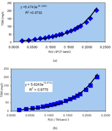
(20) increasing reflectance [Curran et al., 1987; Novo et al., 1989]. Since then, many empirical models have been tested, including: R = A + Bρ [Moreno-Madrinan et al., 2010] R = A + Blgρ or ρ = A + Blg R [Doxaran et al., 2002b] lgρ=A + BlgX [Tassan, 1993] lgρ=A + B(R(555)+R(645)) + C(R(488)/R(555)) [Zhang et al., 2010] Where R is reflectance, ρ is concentration of sediment.. In the study of Miller et al. (2004) the utility of MODIS 250 m Band 1 data for analyzing complex coastal waters were examined in the northern Gulf of Mexico. The MODIS 250m Band 1 data was chosen because it provides coverage in the red spectral region (620–670 nm) at sensitivity sufficient for coastal water studies. Surface water samples were obtained from three different environments in the northern Gulf of Mexico (Figure 1.4.1.1) to obtain the SSC value.. Figure 1.4.1.1 Location map of the three study areas (Lake Pontchartrain, Mississippi River Delta and Mississippi Sound) in the northern Gulf of Mexico. 11.

(21) Then, based on the formula TSM = A + B R (where TSM: total suspended matter; R: reflectance), an empirical relationship between TSM and reflectance of Terra MODIS 250m Band 1 was ascertained (Figure 1.4.1.2). Results showed a significant relationship (r2=0.89, n=52).. Figure 1.4.1.2 Empirical relation between total suspended matter (TSM) and reflectance of Terra MODIS 250m Band 1 (O) Mississippi Sound 16 May 2001; (●) Mississippi River Delta 17 March 2002; (□)Mississippi River Delta 15 July 2003; (■) Lake Pontchartrain 19 May 2002; (Δ) Lake Pontchartrain 23 May 2002; (▲)Mississippi River Delta 20 October 2003. 1.4.2 Analytical Approach. Although these empirical models proved to be reasonably accurate when applied to satellite images concurrent with calibration data sets, their accuracy may be reduced where the conditions are outside of the calibration data set. This is because they depend fundamentally on the specific data and conditions under which they are calibrated. Analytical approaches have overcome such limitations with models based on knowledge of the physical relationship between reflectance and SSC. Bio-optical 12.

(22) models which are based on knowledge of the in-situ inherent optical properties (IOPs), have lead to the development of sufficiently reliable multi-temporal algorithms for SSC retrieval. Such models use an algorithm that has been developed from laboratory analysis data of IOPs and its constituents. The average value of the Specific Inherent Optical Properties (SIOP) is used as the input of the model. Case studies have shown that such methodology was suitable for SSC retrieval with sufficient accuracy [Ambarwulan and Hobma, 2004; Haltrin and Arnone, 2003]. Based on the knowledge that the remote sensing reflectance is a function of the water depth, the properties of the matter suspended in it, and of the optical properties of the bottom, theoretical and physically-based approaches were developed. These methods link the directional remote sensing reflectance in the nadir direction to the controlling physical factors in a direct and controllable manner making SSC retrieval possible [Lee et al., 1998; 1999]. Volpe et al (2011) developed a SSC retrieval algorithm based on a physically based radiative transfer model which applied to satellite measured reflectance at 650nm and returned an acceptable result.. Ambarwulan et al. (2004) used an optical method to retrieve SSC of Teluk Banten (Banten Bay, latitude of 05°50′00″ -06°04′00″S and longitude of 106°05′00″ 106°17′00″E) from Landsat TM 5 (27 May 1995; 14 June 1996 and 30 January 1997) and SPOT HRV (12 June 1990; 14 April 1996; and 8 October 1997).. In this study the following optical models have been used for retrieving SSC.. a=aw+apig×TCHL+atr×TSM+aCDOM×CDOM440; bb=0.5×bw+btr×TSM. Where: CHL: chlorophyll TSM: Total Suspended Matter. 13.

(23) aw: the absorption of pure water bw: the backscattering of pure water apig: the specific absorption of phytoplankton pigment atr: the specific absorption of tripton aCDOM: the specific absorption of CDOM CDOM440: the CDOM absorption of 440 nm btr: the specific scattering of tripton. The average value of SIOP for CDOM absorption, tripton absorption, phytoplankton absorption and seston scattering has been used for the entire study area (Figure 1.4.2.1).. Figure 1.4.2.1 The average SIOP of Teluk Banten. Finally the relation was built for SSC retrieval (Figure 1.4.2.2).. 14.

(24) (a). (b) Figure 1.4.2.2 (a) Algorithm based on SPOT HRV; (b) algorithm based on LandSat TM5. This study proved that optical methodology can be used to map the spatial distribution of SSC with sufficient accuracy. However the accuracy of this model is heavily reliant on accurate spectral models for the absorption coefficient of each individual constituent presented in the water such as SSC and total chlorophyll-a (TCHL) concentration. This method is also time-consuming as it requires the processing of large remote sensing satellite data sets.. 15.

(25) 1.4.3 Non-linear Optimisation Approach. Both the empirical approach and the analytical approach need in-situ measurements. Unfortunately, in-situ measurements are often unavailable for direct image calibration and the IOPs of optically active constituents (specific scattering and absorption coefficients) are usually unknown. By using an optical mathematical approach Rodný et al. (2010) examined the possibility of retrieving SSC using only image-derived information. The core idea of using only remote sensing data to retrieval coastal water SSC is based on using an exponential function to relate reflectance and SSC, with SSC replaced by a linear relationship between SSC and reflectance in the near-infrared domain. Results show that spatial patterns of suspended sediments can be retrieved from remotely sensed data even if ground measurements are absent.. Figure 1.4.3.1: Comparison of simulated and in-situ measurements of suspended sediment concentrations. This study uses two SSC retrieving methods. One is non-linear optimisation which uses only remote sensing data to retrieve near-shore coastal SSC. The other is a quasianalytical method which uses a quasi-analytical algorithm for retrieving the absorption and backscattering coefficients from remote sensing reflectance of near-shore coastal waters and applying these to build the relationship between reflectance and the inherent optical properties of water. The quasi-analytical approaches have similar accuracy to 16.

(26) analytical approaches while the calculation efficiency is comparable to empirical approaches [Lee et al., 2002].. 1.5 Rivers. There are four rivers which discharge into the study area: the Whanganui, Whangaehu, Rangitikei and Manawatu rivers. Beginning on the northern slopes of Mount Tongariro, the Whanganui River is a major river in the North Island of New Zealand. With a length of 290 km, the Whanganui is the country's third-longest river. It flows to the north-west before turning south-west at Taumarunui. From here it runs through the rough, bush clad hill country of the King Country before turning south-east and flowing past the small settlements of Pipiriki and Jerusalem, finally reaching the coast at Whanganui [Travel Media, 2012]. The Whangaehu River starts on the slopes of Mount Ruapehu and begins as the melt water from a small glacier. It flows for 135 kilometres southward to the South Taranaki bight, near the settlement of Whangaehu [Poole, 1983]. Another large river that arises from the Taupo basin is the Rangitikei River which is 185 kilometres long. It flows south from the Central Plateau, past Taihape, Mangaweka, Hunterville, Marton, and Bulls to the South Taranaki bight at Tangimoana, 40 kilometres southeast of Whanganui. The Whanganui and Rangitikei rivers are deeply entrenched. They have cut down through soft sedimentary rocks as the country they drain has been uplifted. With a length of 180 km the Manawatu River is also a major river of the southern North Island of New Zealand. The river has its headwaters to the northwest of Norsewood in the Ruahine Ranges of southern Hawke's Bay. It initially flows eastward before turning south-west near Ormondville, flowing for 40 km before turning north-west near Woodville. At this point the river enters the Manawatu Gorge. It then turns again, flowing south-west, through Palmerston North and finally entering the Tasman Sea at Foxton Beach. At the river mouth, the Manawatu River has an average discharge of 102 cubic metres per second [Travel Media, 2012].. 17.

(27) 1.6 Horizons Regional Council. The daily mean flow and sediment load (flow) data used in this study has been provided by the Horizons Regional Council (Horizons). Horizons manages the land, air and water of the Tararua, Manawatu, Horowhenua, Rangitikei, Whanganui and Ruapehu districts, Palmerston North City as well as parts of the Waitomo, Taupo and Stratford districts. Overall the authority is responsible for 22,215 sq km of land or 8.1% of New Zealand’s total land area. The four Horizons’ river monitoring stations used in this study are: Whanganui River at Te Rewa, Whangaehu River at Kauangaroa, Rangitikei River at Onepuhi and Manawatu River at Teacher’s College, Palmerston North [Horizon Council 2012]. (Figure 1.6.1). Figure 1.6.1 Four river monitoring stations. 18.

(28) 2 Method. 2.1 Study Area. The study area is the near-shore zone of the south-west coast of the North Island, New Zealand. (Figure 2.1.1) This is ideal for this research as four major rivers discharge here; the Whanganui, Whangaehu, Rangitikei and Manawatu rivers. Flow data of four river monitoring stations were used to determine flood time. They are: Whanganui River at Te Rewa, Whangaehu River at Kauangaroa, Rangitikei River at Onepuhi and the Manawatu River at Teacher’s College, Palmerston North. Satellite images were chosen based on the river flow dataset.. Figure 2.1.1 Satellite image of South West coast of North Island, New Zealand. 2.2 Data Download. Remote sensing data collected by the Moderate Resolution Imaging Spectroradiometer (MODIS) sensor are used in this paper. Terra/Aqua MODIS level 1B calibrated 19.

(29) Radiance 250M Band 1 & 2 (which contains reflectance and radiance data) were downloaded. through. NASA. internet. servers:. LAADS. Web. (http://ladsweb.nascom.nasa.gov).. This data was accessed by first selecting MODIS, Terra (or Aqua) level 1 products and MOD02QKM (or MYD02QKM) – Level 1B Calibrated Radiances – 250m (Figure 2.2.1) as the product selection. In addition “latitude/longitude” was selected along with the region of interest in the spatial selection section (Figure 2.2.2).. Figure 2.2.1 LAADS Product Selection. 20.

(30) Figure 2.2.2 Select download region. 2.3 Georeferencing and Bow Tie Effect Correction. Before analysis MODIS data need first to be georeferenced and corrected for the bow tie effect. (Figure 2.3.1) Because of the larger ground-sampled size of the edge pixels in relation to the ground sample size of the image pixels located in the centre of the scan, the data collected by the MODIS sensors aboard the Terra (EOS AM) and Aqua (EOS PM) satellites include a so-called bow tie effect.. 21.

(31) Figure 2.3.1 Georeferencing and bow tie effect correction. 2.4 Atmospheric Correction. This study used ENVI FLAASH to correct the atmospheric effect. ENVI FLAASH is an atmospheric correction tool that corrects wavelengths in the visible through nearinfrared and shortwave infrared regions, up to 3 μm. It supports hyperspectral sensors (HyMAP, AVIRIS, HYDICE, HYPERION, Probe-1, CASI, and AISA) and multispectral sensors (ASTER, AVHRR, GeoEye-1, IKONOS, IRS, Landsat, MODIS, QuickBird, RapidEye, SeaWiFS, SPOT, and WorldView-2). The input image for ENVI FLAASH must be a radiance image in band-interleaved by-line (BIL) or bandinterleaved-by-pixel (BIP) format. The data type may be floating-point, 4-byte signed integers, 2-byte signed integers, or 2-byte unsigned integers. It also requires input data to be floating-point values in units of μW/cm2 * nm* sr.. 22.

(32) Figure 2.4.1 FLAASH Atmospheric Correction Model Input Parameters. 2.5 SSC Retrieve. 2.5.1 Non-linear Optimisation. Non-linear optimisation is an approach that uses only remote sensing satellite data to retrieve near-shore coastal water SSC. The core idea is based on using an exponential function to relate reflectance and SSC, with SSC replaced by a linear relationship between SSC and reflectance in the near-infrared domain [Onderka and Rodny, 2010]. In the visual domain (400 – 700 nm) the relationship of SSC and reflectance can be modelled by using the following model [Schiebe et al., 1992]:. (2.5.1.1). 23.

(33) Where: Ri: reflectance in i th spectral band; Ai: contribution of the atmospheric reflectance and air-water specular reflection; Bi: asymptotic value of Ri; SSC: concentration of suspended sediments (mg/L); Si: saturation concentration (mg/L); i: identifier of the spectral band being analyzed.. Reflectance recorded in the near infrared domain (700 – 900nm) has a near linear relationship with a broad range of SSC [Schiebe et al., 1992]. This relationship can be described by the following model [Doxaran et al., 2004; Tolk et al., 2000]:. SSC=α+β×R(NIR). (2.5.1.2). Where: α and β are empirically derived constants R(NIR): reflectance of near infrared. The reason for using remote sensing reflectance (which is the ratio between incident irradiance and water leaving radiance) in formula 1 and 2 is that under varying illumination conditions this optical property is the most practical of MODIS data for retrieval SSC. The reflectance value also provides a practical basis for inter-image comparison [Onderka and Rodny, 2010].. Based on formulae 2.5.1.1 and 2.5.1.2: (2.5.1.3). 24.

(34) where: Rvisual: at-sensor radiance recorded in the visual domain (R, G or B); R(NIR): at-sensor radiance in the near-infrared band; Ai: contribution of the atmosphere and air-water specular reflection; Bi: asymptotic value of DNs in i-th visual band; Si: saturation concentration (mg/L); α and β are empirically derived constants. In formula 2.5.1.3 reflectance was replaced by radiance. This is because the empirically derived parameters already involve the atmospheric and illumination effects.. Finally a non-linear optimisation method is used to identify the unknown parameters of formula 2.5.1.3, where the “objective function” which needs to be minimized is:. Weighted error=. Where: Rvisual is the radiance value; RFIT is the corresponding radiance value on the best-fit curve; N denotes the number of analyzed pixels.. In this study the Microsoft Excel programme (Excel) was used to calculate unknown parameters of the above formulas. This was achieved by firstly exporting the value of 6,000 points of each image to an ASCII file (ROI Tool: File—Out put ROIs to ASCII) and then importing the ASCII file to an Excel worksheet. Finally an optimisation macro (Excel plug in) was used to calculate the unknown parameters (A, B, α, β and s) of the sediment concentration model [Foxes Team, 2011]. The optimisation macro (Optimiz) was developed for performing the optimisation task directly on an Excel worksheet. It 25.

(35) progresses by iterations; starting from an approximate trial solution an algorithm will gradually refine the working estimate until a prefixed precision has been reached. This can define any relationship by using the standard Excel built-in functions and equations that relate them. The optimisation macros will directly update the cells containing the parameters to be changed and the related variables to be optimised.. Before starting the optimising procedure, the initial values of the unknown parameters have to be assigned in advance. After running the Optimiz tool, optimisation propagates in iterative runs, minimizing the predefined objective function (weighted error) at each run. As a result, each iteration is updated by the parameters obtained in the previous run, until a final solution is reached when the objective function is minimized (Figure 2.2.1.1).. Figure 2.5.1.1 Optimizing Excel worksheet. 26.

(36) 2.5.2 Quasi-analytical. A quasi-analytical algorithm was used for retrieving the absorption and backscattering coefficients from remote sensing reflectance of near-shore coastal waters. The above surface reflectance is first converted to below surface reflectance using the following formulae:. (2.5.2.1). Where: Below surface remote sensing reflectance Above surface remote sensing reflectance Radiance transmittance from below to above the surface Irradiance transmittance from above to below the surface Refractive index of water Water to air internal reflection coefficient Ratio of upwelling irradiance to upwelling radiance evaluated below the surface. Mobley (1995) has suggested that for optically deep waters and a nadir-viewing sensors:. 0.52 and. 1.7.. In general, on the basis of theoretical analyses and numerical simulations of the radiative transfer equation, rrs is a function of the absorption and backscattering coefficients.. 27.

(37) (2.5.2.2) With (2.5.2.3). Where Below surface remote sensing reflectance spectra at u Ratio of backscattering coefficient to the sum of absorption and backscattering coefficients a Absorption coefficient of the total Backscattering coefficient of the total. For nadir viewed. , Gordon et al. found that. case1 waters, while Lee et al. suggested that. 0.0949 and. 0.0794 for oceanic. 0.084 and. 0.17 worked better for. near-shore coastal waters.. Because if:. Then:. (. So from equation 2.5.2.2:. ) Because. must be positive:. 28. ).

(38) As. is a simple ratio of backscattering coefficient to the sum of absorption and. backscattering coefficients, knowing a will lead to:. Figure 2.5.2.1 Absorption coefficient variations at different wavelengths. For each wavelength, the total absorption coefficient can be expressed as:. (2.5.2.4). Where: Absorption coefficient of the total at Absorption coefficient of pure water at Contribution that is due to dissolved and suspended constituents at. As can be seen from Figure 2.5.2.1,. is very small at longer wavelengths (MODIS. Band 1). Based on this, the absorption coefficient of water can be approximated by that of pure water at the longer wavelengths and hence the backscattering coefficient at that wavelength can be calculated using the above equations. 29.

(39) The relationship between varying levels of SSC and spectral reflectance of water is derived from Lodhi’s paper [Lodhi et al., 1997]. Lodhi et al (1997) pointed out that this relationship varies between different suspended sediment types. Based on the sample that was collected for laboratory experiments (section 2.6) the suspended sediment type in this study belongs to ‘silty soil’ category of Lodhi’s paper. Table 2.5.2.1 was used to establish the empirical relation between the backscattering coefficient and SSC using EXCEL. [Pegau and Zaneveld, 1993; Pegau et al., 1997; Pope and Fry, 1997; Sogandares and Fry, 1997].. SSC (mg/l). reflectance (%). Sub-surface reflectance. g0. g1. u(λ). Absorption Coefficient. Backscattering Coefficient. 0 50 100 150 200 250 300 350 400 450 500 550 600 650 750 850 950 1000. 1.9 4 6.5 8 9.1 9.8 10.5 11 11.6 11.7 12.1 12.6 13 13.05 13.08 13.1 13.2 13.5. 0.034401593 0.068027211 0.103092784 0.12195122 0.134874759 0.142732304 0.150322119 0.155586987 0.1617401 0.162748644 0.166735566 0.171615364 0.175438596 0.175911572 0.176194838 0.176383466 0.177324019 0.18012008. 0.084 0.084 0.084 0.084 0.084 0.084 0.084 0.084 0.084 0.084 0.084 0.084 0.084 0.084 0.084 0.084 0.084 0.084. 0.17 0.17 0.17 0.17 0.17 0.17 0.17 0.17 0.17 0.17 0.17 0.17 0.17 0.17 0.17 0.17 0.17 0.17. 0.26616664 0.432056871 0.569927223 0.635209943 0.677289054 0.701961646 0.72519928 0.74099767 0.759147128 0.762090831 0.773644614 0.787610303 0.798421835 0.800547155 0.801076597 0.803712574 0.803712574 0.811509996. 0.3513 0.3513 0.3513 0.3513 0.3513 0.3513 0.3513 0.3513 0.3513 0.3513 0.3513 0.3513 0.3513 0.3513 0.3513 0.3513 0.3513 0.3513. 0.127419038 0.267247847 0.465538496 0.61171967 0.737290282 0.827407354 0.92708093 1.005058455 1.10726679 1.12531396 1.200684276 1.302735036 1.391448274 1.403020944 1.410018572 1.41470639 1.43842238 1.512459308. Table 2.5.2.1 Relationship between the backscattering coefficient and SSC. with. SSC =. Where: b: Backscattering coefficient at 645nm. 30. 0.9602.

(40) Figure 2.2.2.2 Empirical relation between backscattering coefficient and SSC. This relationship is applied to convert the backscattering coefficient (which is retrieved from satellite measured water reflectance) to suspended sediment concentration.. 31.

(41) Data processing Demo Above surface reflectance spectra: R R= 0.04. Below surface reflectance spectra: r. (. 1.7). 0.52 and. =0.068027211. Ratio of b to (a+b): u. (. 0.084 and. 0.17) =0.432056871. Backscattering coefficient: b. (Check value of a from table 1) =0.267247847. SSC =. SSC=683.15×0.26724784731177×0.2672478472+931.79×0.267247847-119.04≈59. 32.

(42) 2.6 Laboratory Experiments. Laboratory experiments were carried out to study the relationship between optical parameters and SSC. An ASD FieldSpec Pro was used to do the spectral measurement.. 2.6.1 Instruments:. FieldSpec Pro: FieldSpec Pro manufactured by Analytical Spectral Devices, Inc. This offers superior signal-enhancing features and high resolution with a 350 - 2500 nm spectral range. ASD Pro Lamp: This is a 14.5 Volt 50 Watt Lamp that is tripod mountable and adapted especially for indoor lab diffuse reflectance measurements over the region 350 - 2500 nm. This lamp cannot be used closer than 0.5m or at an angle of less than 45°.. Fibre optic cables. Foreoptic: Lenses which limit the field-of-view to 8 degrees. White reference standard: A material with approximately 100% reflectance across the entire spectrum.. 33.

(43) 2.6.2 Instruments Set Up. For measurement with the lens foreoptics, it is important to accurately define the instantaneous field of view (IFOV) of the sensor. The FOV is approximately circular and 8° (Figure 2.6.2.1. ). H=. (2.6.2.1). Where: H: distance between foreoptic and the surface measured (Figure 2.6.2.1 OF) r: radius of the measured area (Figure 2.6.2.1 EF) x: Field-of-view of Foreoptic (Figure 2.6.2.1. ). In this experiment the radius of the measured area is 4cm and the height of the foreoptic is H plus the height of water.. ASD Pro Lamp height: 85 cm (Figure 2.6.2.1 HI). 34.

(44) Figure 2.6.2.1 Instruments set up. 2.6.3 Spectral Measurements. Reflectance spectra of different backgrounds (different papers and different containers), different water height (pure and salt water), different light angle and different SSC are generated using FieldSpec Pro. When the graph on the computer screen remains stable, a scan can be collected. The computer can be used to automatically save each file. Each of following results used a mean value of ten measures.. 35.

(45) 3 Results and Discussion:. 3.1 Laboratory Experiments. Figure 3.1.1 Reflectance spectra of different papers. As expected, black paper absorbed the most light energy and had a steady reflectance spectra at the visible area (400 – 700nm) while the reflectance spectra of blue paper had a peak at the visible blue area.. 36.

(46) Figure 3.1.2 Reflectance spectra of different containers on black background. Figure 3.1.2 indicates that the white container reflects more light than the blue or green containers. In the visible area the reflectance value of the white container is above 30 percent, while the peak reflectance value of blue and green container remains around 13 percent.. 37.

(47) Figure 3.1.3 Reflectance spectra of different depths of pure water (white container on the black background). Figure 3.1.3 shows that as the depth of water increases the reflectance value drops. Water at depth of 5cm has reflectance value of 32% compared to water with a depth of 20cm which has reflectance value of 22% at 600nm. This is because with lower water depth more light reaches the bottom and the bottom has a higher reflectance than water. Beyond 920 nm reflectance is near zero which indicates that water absorbs most of the energy at the longer wavelengths.. 38.

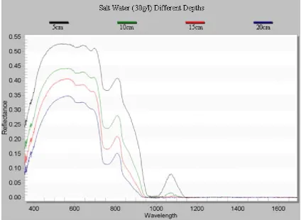
(48) Figure 3.1.4 Reflectance spectra of different depths of salt water (30g/l) (white container on the black background). As can be seen from Figure 3.1.4 the reflectance spectra of salt water has similar properties to the reflectance spectra of pure water. However in the visible area (400 – 700nm) the reflectance spectra at the varying salt water depths are very close to each other, as the black background has a very low reflectance (Figure 3.1.1).. 39.

(49) Figure 3.1.5 Reflectance spectra of different depths of salt water (30g/l) (white container on the white background). Compared with Figure 3.1.4 the reflectance spectra of salt water on a white background has a higher value. Water at a depth of 5cm returns a value of 53 percent on the white background compared with 23 percent from water of the same depth on the black background at 600nm. This indicates that light reaches the bottom and that the white background has higher reflectance value than black background.. 40.

(50) Figure 3.1.6 Reflectance spectra of different light angle (pure water 20cm water height, white container on the white background). Figure 3.1.6 shows that light angle also has impact on the reflectance spectra. Between 400nm – 920nm the reflectance of light at a 65° angle has the highest value while the reflectance of light at a 35° angle has the lowest value as would be expected. By increasing the light angle from 35 degrees to 65 degrees, the value of reflectance goes up from 18percent to 45percent.. 41.

(51) Figure 3.1.7 Reflectance spectra of different light angle (pure water 15cm height, white container on the white background). Figure 3.1.7 indicates when water depth drops to 15 cm reflectance the value increases as more light reaches the bottom. As the light angle has a significant impact on the reflectance spectra, the light angle been adjusted before each SSC reflectance experiment to simulate the solar angle at the time the satellite image was captured.. 42.

(52) Figure 3.1.8 Reflectance spectra of different SSC (salt water 20cm height, white container on the black background). Figure 3.1.8 indicates that reflectance at visible to near infrared bands is sensitive to changes of SSC. Thus bands of remote sensing satellite visible to near infrared data are used commonly for retrieving near-shore coastal SSC. As can be seen from the results, SSC reflectance spectra has very similar shape with the measurements reported in other papers [Kou et al., 1993; Pegau and Zaneveld, 1993; Pegau et al., 1997; Pope and Fry, 1997; Sogandares and Fry, 1997]. However, as in this experiment, the depth of water is not deep enough which means that the reflectance of the bottom is able to be measured. As the bottom has a higher reflectance, when the SSC value increases the reflectance of water with sediment becomes the dominant part of total reflectance. This is caused because as the SSC value increases, the reflectance value decreases.. 43.

(53) 3.2 SSC Retrieval To illustrate the two methods used in this paper, nine Terra/Aqua MODIS 250m remote sensing images of the south-west coast of the North Island, New Zealand were used to derive SSC maps. Results indicate that the SSC maps derived from the two retrieval approaches are very similar.. 44.

(54) 3.2.1 SSC Map. Figure 3.2.1.1 Terra 18 January. Date. Manawatu at Teachers College 18/01/2011 12170. Rangitikei at Onepuhi 8030. Whangaehu at Kauangaroa 10216. Whanganui at Te Rewa 46435. Table 3.2.1.1 Daily mean flow data (l/s) of four river monitoring stations Date. Manawatu at Rangitikei at Whangaehu at Whanganui Teachers College Onepuhi Kauangaroa at Te Rewa 18/01/2011 9.51 26.2 1 73.2 3 Table 3.2.1.2 Sediment Load (Kg/m ) of four river monitoring stations. 45.

(55) Figure 3.2.1.2 Aqua 19 January. Date. Manawatu at Rangitikei at Whangaehu at Whanganui Teachers College Onepuhi Kauangaroa at Te Rewa 19/01/2011 14920 8036 15849 92007 Table 3.2.1.3 Daily mean flow data (l/s) of four river monitoring stations Date. Manawatu at Rangitikei at Whangaehu at Whanganui Teachers College Onepuhi Kauangaroa at Te Rewa 19/01/2011 48.3 25.1 298 608 3 Table 3.2.1.4 Sediment Load (Kg/m ) of four river monitoring stations. 46.

(56) As can be seen from Figure 3.2.1.1 and Figure 3.2.1.2, during times of normal flow there are no obvious high sediment concentrations around the river mouths and high SSC area is only seen along the coastal line. This is despite the fact that the amount of sediment carried by each river is different, for example on 19 January 2011 the sediment load of the Manawatu River was only 48.3 kg/m3 compared with 608 kg/m3 in the Whanganui River (Table 3.2.1.4). This indicates sediment from each river is spread evenly in the coastal area.. 47.

(57) Figure 3.2.1.3 Terra 24 January. Date. Manawatu at Rangitikei at Whangaehu at Whanganui Teachers College Onepuhi Kauangaroa at Te Rewa 24/01/2011 520513 577480 560954 2340586 Table 3.2.1.5 Daily mean flow data (l/s) of four river monitoring stations Date. Manawatu at Rangitikei at Whangaehu at Whanganui Teachers College Onepuhi Kauangaroa at Te Rewa 24/01/2011 18000 60300 34600 157000 3 Table 3.2.1.6 Sediment Load (Kg/m ) of four river monitoring stations 48.

(58) Figure 3.2.1.4 Aqua 25 January. Date. Manawatu at Rangitikei at Whangaehu at Whanganui Teachers College Onepuhi Kauangaroa at Te Rewa 25/01/2011 263735 226019 185756 1128549 Table 3.2.1.7 Daily mean flow data (l/s) of four river monitoring stations Date. Manawatu at Rangitikei at Whangaehu at Whanganui Teachers College Onepuhi Kauangaroa at Te Rewa 25/01/2011 2660 6600 2040 27400 3 Table 3.2.1.8 Sediment Load (Kg/m ) of four river monitoring stations 49.

(59) Figure 3.2.1.5 Daily mean flow. Figure 3.2.1.6 Sediment Load 50.

(60) As can be seen from the bar charts (Figure 3.2.1.5 & 3.2.1.6), from 24 January 2011 to 25 January 2011 the daily mean flow data dropped by about 50percent and sediment load went down significantly. The expected sediment load of the Whanganui River decreased by about 80 percent while the other three rivers sediment loads dropped by about 90percent. Thus less sediment was deposited in the near-shore coastal area. As a result on 24 January 2011 high SSC areas are seen around the river mouths of all four rivers on the SSC map. On 25 January 2011 only one obvious high SSC area can be seen around mouth of the Whanganui River.. 51.

(61) Figure 3.2.1.7 Terra 28 January. Date. Manawatu at Rangitikei at Whangaehu at Whanganui Teachers College Onepuhi Kauangaroa at Te Rewa 28/01/2011 56366 35740 31551 171578 Table 3.2.1.9 Daily mean flow data (l/s) of four river monitoring stations Date. Manawatu at Rangitikei at Whangaehu at Whanganui Teachers College Onepuhi Kauangaroa at Te Rewa 28/01/2011 222 355 120 1030 Table 3.2.1.10 Sediment Load (Kg/m3) of four river monitoring stations. 52.

(62) 2500000. Daily mean flow (l/s). 2000000 1500000 18/01/2011 24/01/2011. 1000000. 28/01/2011 500000 0 Whanganui. Whangaehu. Rangitikei. Manawatu. Rivers. Figure 3.2.1.8 Daily mean flow. Figure 3.2.1.9 Sediment Load As the bar charts show after four days of flood (24 January 2011) the daily mean flow and sediment load values are almost back to normal levels (18 January 2011). Thus it can be seen that on 28 January 2011 there are no obvious areas of high SSC on the SSC map, but on that day the average SSC value is higher than on 18 January 2011. This indicates that the suspended sediment introduced by the flood has spread to a larger coastal area.. 53.

(63) Figure 3.2.1.10 Terra 11 April. Date. Manawatu at Rangitikei at Whangaehu at Whanganui Teachers College Onepuhi Kauangaroa at Te Rewa 11/04/2011 39849 14010 15466 75265 Table 3.2.1.11 Daily mean flow data (l/s) of four river monitoring stations Date. Manawatu at Rangitikei at Whangaehu at Whanganui Teachers College Onepuhi Kauangaroa at Te Rewa 11/04/2011 115 69.8 16 189 Table 3.2.1.12 Sediment Load (Kg/m3) of four river monitoring stations. 54.

(64) Figure 3.2.1.11 Aqua 12 April. Date. Manawatu at Rangitikei at Whangaehu at Whanganui Teachers College Onepuhi Kauangaroa at Te Rewa 12/04/2011 34055 12431 14927 67649 Table 3.2.1.13 Daily mean flow data (l/s) of four river monitoring stations Date. Manawatu at Rangitikei at Whangaehu at Whanganui Teachers College Onepuhi Kauangaroa at Te Rewa 12/04/2011 84.2 56.9 14.4 148 Table 3.2.1.14 Sediment Load (Kg/m3) of four river monitoring stations. 55.

(65) Figure 3.2.1.12 Terra 28 April. Date. Manawatu at Rangitikei at Whangaehu at Whanganui Teachers College Onepuhi Kauangaroa at Te Rewa 28/04/2011 500223 133256 46326 232784 Table 3.2.1.15 Daily mean flow data (l/s) of four river monitoring stations Date. Manawatu at Rangitikei at Whangaehu at Whanganui Teachers College Onepuhi Kauangaroa at Te Rewa 28/04/2011 14000 5070 203 1300 Table 3.2.1.16 Sediment Load (Kg/m3) of four river monitoring stations. 56.

(66) Figure 3.2.1.13 Aqua 29 April. Date. Manawatu at Rangitikei at Whangaehu at Whanganui Teachers College Onepuhi Kauangaroa at Te Rewa 29/04/2011 263157 87360 29375 136354 Table 3.2.1.17 Daily mean flow data (l/s) of four river monitoring stations Date. Manawatu at Rangitikei at Whangaehu at Whanganui Teachers College Onepuhi Kauangaroa at Te Rewa 29/04/2011 3740 1730 78.4 577 3 Table 3.2.1.18 Sediment Load (Kg/m ) of four river monitoring stations. 57.

(67) The derived SSC maps show that the extent of high SSC areas has a high correlation to the flow rate of the contributing river, while the value of SSC is related to the value of sediment load. As the above SSC maps show, the suspended sediment spreads to the larger coastal area at different rates after flooding. This is because the coastal environment consists of constantly changing conditions, caused by the forces of wind, waves, currents and tides. In the coastal area sediment transport is mainly due to currents and tides.. The types of suspended sediment can differ from river to river and during flood sediment types can also change within the same river. Normally the largest sediment a river can carry is sand and gravel, but larger floods can carry cobbles and even boulders. As discussed in the first section, all four rivers discharging to the study area start in different locations and follow a unique flow path to the ocean. For instance the Whanganui River starts on the northern slopes of Mount Tongariro which is one of the three active volcanoes of the Central Plateau. The Whangaehu River starts on the slopes of Mount Ruapehu and begins as the melt water from a small glacier. The headwaters of Rangitikei River are to the southeast of Lake Taupo in the Kaimanawa Ranges and the Manawatu River has its headwaters to the northwest of Norsewood in the Ruahine Ranges of southern Hawke's Bay. As a result these rivers contain different types of sediment.. When using a quasi-analytical method to retrieve SSC, types of sediment should be taken into account. Liew et al. (2009) point out that the linear relationship between SSC and backscatter is slightly variable and dependant on the suspended sediment type in that area. Thus identification of the type of sediment the river brings to the coastal area can greatly improve the accuracy of SSC mapping.. 58.

(68) 3.2.2 Total Sediment Calculation. There are many factors that can affect the suspended sediment distribution in the coastal water column, such as type of sediment, sea water temperature, salinity and density. The variety and complexity of suspended sediment transportation make it difficult to construct a picture based only on theoretical models. These models usually contain many assumptions and need to be checked against in-situ data sets. Thus, in order to calculate the total suspended sediment in the study area the assumption is made that in the shallow water (<10 m) suspended sediment is evenly distributed in the water column [Condie and Sherwood, 2006; Novo et al., 1989]. Another assumption made in this calculation is that the satellite can measure high turbidity sea water up to 1m in depth. Finally total suspended sediment of the study area was calculated using SSC maps and a DEM file (which created from a bathymetric contour map).. Two contour maps. Georeferencing & Mosaic two contour files into one file. Digitising contour map to shape file. Create TIN from shape file. Create DEM from TIN. Figure 3.2.2.1 From contour maps to DEM 59.

(69) (a). (b). (c). (d). Figure 3.2.2.2 Contour maps (a) Wanganui river mouth; (b) Whangaehu river mouth; (c) Rangitikei river mouth; (d) Manawatu river mouth. Figure 3.2.2.3 TIN of the study area. 60.

(70) Figure 3.2.2.4 DEM of the study area. 61.

(71) Figure 3.2.2.5 Near-shore high SSC area (within the red line) 11 April 2011. Near-shore coastal area Total sediment (kg). 167119944. Area (m3). 1390000. Table 3.2.2.1 High suspended sediment area 11 April 2011. 62.

(72) In order to calculate the total sediment and area of the study area, ENVI band math was first used to generate the SSC value in the whole water column (surface SSC value (SSC maps). water depth (DEM)). Then the ENVI statistics tool was used to calculate. the number of pixels and pixel mean value of the interest area. As each pixel of the data set used in this study covers 250. 250 m2, the total area can be calculated using the. following formulae: Area Where p: numbers of pixel. Value of total sediment can be calculated using the following formulae: Total sediment Where p: numbers of pixel pm: pixel mean value of the interest area. As can be seen from Figure 3.2.1.18, the SSC value along the coast line is very high even during the non-flood time. As the pixels along the coast line are not very pure this may have caused this phenomenon. As each pixel of the data set used in this study covers 250. 250m2 it is possible that the pixels along the coast line contains. information about the land which means that the SSC values along the coast line are not as accurate as the rest of the near-shore coastal area.. 63.

(73) Figure 3.2.2.6 Near-shore high SSC area (within the red line) 24 January 2011. a. Whanganui. b. Rangitikei. c. Manawatu. Total sediment (kg). 250680. 25668. 100272. Area (m3). 1123500. 246500. 556000. Table 3.2.2.2 High suspended sediment area 24 January 2011 64.

(74) Figure 3.2.2.7 Near-shore high SSC area (within the red line) 29 April 2011. a. Whanganui. b. Rangitikei. c. Manawatu. Total sediment (kg). 6267. 6267. 269680. Area (m3). 163000. 139500. 679500. Table 3.2.2.3 High suspended sediment area 29 April 2011. 65.

(75) 4 Conclusion and future work. The results indicate that useful SSC maps can be derived from satellite images. Both methods used in this paper do not require the availability of external data and thus can be used for monitoring near-shore coastal water SSC on a regular basis. As can be seen from the figures, the SSC maps derived using the two retrieval approaches are very similar. The extent of high SSC area around the river mouths has a strong correlation to the flow rate and sediment load of that river.. Mapping SSC of coastal areas is important to many scientific and environmental studies, since the SSC distribution can be used as indicator of biomass primary production, erosion and deposition processes, transport of nutrients and micropollutants. Take erosion study as an example, during the last two centuries much of New Zealand’s indigenous forest has been converted into pastoral land and increased erosion and has lead to a dramatic loss of soil. As a result sediment loads in the rivers have increased. Thus it is necessary to monitor sediment discharge to the ocean. As discussed in this paper, total sediment in the coastal area can be calculated using satellite imagery. And the result can be used to help understand how much sediment is transported from the river during a specific time.. To gain a more accurate SSC map, types of sediment should be better identified when using the quasi-analytical method because the linear relationship between SSC and backscatter is slightly variable depending on the suspended sediment type in that area. When using the optimising method, the initial values of the unknown parameters must be assigned in advance. The initial values can be selected arbitrarily, however to ensure an accurate result the initial values need to be feasible in their physical interpretation. The physical properties of coastal waters determined though laboratory experiments can be used to improve the performance of the optimising method.. 66.

No results found