SOLUTIONS OF A SINGULARLY PERTURBED SEMILINEAR
REACTION-DIFFUSION PROBLEM∗
NATALIA KOPTEVA† AND MARTIN STYNES‡
Abstract. A semilinear reaction-diffusion two-point boundary value problem, whose second-order derivative is multiplied by a small positive parameterε2, is considered. It can have multiple solutions. The numerical computation of solutions having interior transition layers is analysed. It is demonstrated that the accurate computation of such solutions is exceptionally difficult.
To address this difficulty, we propose an artificial-diffusion stabilization. For both standard and stabilised finite difference methods on suitable Shishkin meshes, we prove existence and investigate the accuracy of computed solutions by constructing discrete sub- and super-solutions. Convergence results are deduced that depend on the relative sizes ofεand N, whereN is the number of mesh intervals. Numerical experiments are given in support of these theoretical results. Practical issues in using Newton’s method to compute a discrete solution are discussed.
Key words. semilinear reaction-diffusion problem, interior layer, Shishkin mesh, error estimates
AMS subject classifications. Primary 65L70, Secondary 34E05, 65L10, 65L11, 65L12, 65L50.
1. Introduction. We are interested in interior-layer solutions of the singularly perturbed semilinear reaction-diffusion boundary-value problem
F u(x)≡ −ε2u′′(x) +b(x, u) = 0 forx∈(0,1),
(1.1a)
u(0) =g0, u(1) =g1,
(1.1b)
whereεis a small positive parameter,b∈C∞([0,1]×R), andg0andg1are given
con-stants. Problems of this type arise frequently in the modelling of stationary patterns in biological and chemical phenomena; see [6] and [14, Chapter 2].
The reduced problem of (1.1) is defined by formally settingε= 0 in (1.1a), viz.,
(1.2) b(x, φ) = 0 forx∈(0,1).
It is often assumed in the numerical analysis literature that bu(x, u)> m >0 for all
(x, u) ∈ (0,1)×R and some positive constant m; then the reduced problem has a unique solutionφ=u0∈C∞(0,1), but this assumption excludes interior layer
tran-sitions between distinct reduced solutions that are important in various applications ([5, Section V], [6, Section 2.3]) and form the subject of this paper. Consequently we shall examine (1.1) under weaker local hypotheses, described in Section 3, that per-mit (1.2) to have more than one solution. No satisfactory numerical method for such problems appears in the literature, but in the present paper we devise and analyse a method that yields an accurate solution of (1.1) by combining a special mesh with a judicious amount of artificial diffusion (cf. [9]).
The structure of the paper is now summarised. We start in Section 2 by discussing the remarkable difficulties that a satisfactory numerical solution of the semilinear problem (1.1) presents owing to the absence of the hypothesis bu >0. A glimpse of
∗This research was supported by Science Foundation Ireland grant 04/BR/M0055. The first
author was also supported by Science Foundation Ireland grant 08/RFP/MTH1536.
†Department of Mathematics and Statistics, University of Limerick, Limerick, Ireland
‡Department of Mathematics, National University of Ireland, Cork, Ireland ([email protected])
these difficulties is given by Figure 2.1, where a standard 3-point difference scheme produces unstable solutions on both an equidistant mesh and an appropriate Shishkin mesh (compare these results with the solutions of the stabilised method that we propose in this paper, which are shown in Figure 2.2). The precise hypotheses that we place on (1.1) are described in Section 3. The numerical methods and a suitable Shishkin mesh are defined in Section 4, where in particular we introduce a stabilised method (4.3) that adds artificial diffusion wherever the mesh size is small compared withε. In Section 5 our main numerical analysis results are stated: existence and error estimates for both the stabilised and standard numerical methods are established. Then Section 6 is devoted to the proofs of these results. This analysis requires many technical details, some of which resemble results already published in the research literature. We hive off this material to a companion technical report [11] in order to minimise the length of the present paper. Numerical experiments that support our theoretical analysis are presented in Section 7.
Remark 1.1. While the analysis and numerical results in this paper are given for the one-dimensional problem (1.1), much of what is here can be generalized to analogues of (1.1)posed in higher dimensions; compare the one-dimensional nonlinear problem discussed in [10] and the extension of this work to the two-dimensional case in [8], where a theoretical analysis and numerical results are presented. The one-dimensional analysis is already so complex that the extra notation required to explain it in two dimensions would only obscure the central ideas that we wish to communicate.
Notation. Throughout the paper, C, C′,C¯ and ¯C′, sometimes subscripted, denote generic positive constants that are independent ofεand of the mesh; furthermore, ¯C
and ¯C′are taken sufficiently large where this property is needed. These constants may take different values in different places. Notation such asf =O(z) means|f| ≤Cz
for someC.
0 1
0 0.5 1 1.5 2 2.5
0 1
[image:2.595.127.390.433.517.2]0 0.5 1 1.5 2 2.5
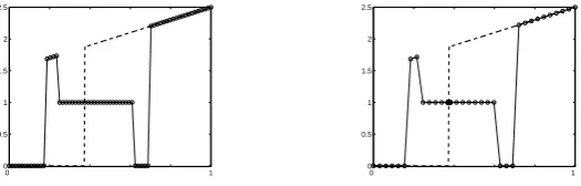
Fig. 2.1. Unstable computed solutions of standard scheme (4.2)versus exact solution (dashed curve) of Example 2.1 withε= 10−3, N = 64 and initial guess the straight line linking the two
boundary values. Left: equidistant mesh. Right: Shishkin mesh (chosen as in Section 7).
2. Numerical intractability of (1.1). To illustrate the substantial difficulties that the numerical solution of the semilinear problem (1.1) presents when we drop the restrictive assumption bu > 0, we consider an example that is a variant of one
appearing in [7].
0 1 0
0.5 1 1.5 2 2.5
0 1
[image:3.595.124.394.96.184.2]0 0.5 1 1.5 2 2.5
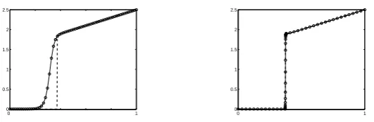
Fig. 2.2. Computed solutions of stabilised scheme (4.3)versus exact solution (dashed curve) of Example 2.1 withε= 10−3,N= 64,Cˆ= 2.5and initial guess the straight line linking the two
boundary values. Left: qualitatively correct solution on equidistant mesh. Right: Shishkin mesh (chosen as in Section 7) yields a computed solution with maximal nodal error 5.19e-2.
A standard 3-point difference scheme—see (4.2) below—on an equidistant mesh and on an appropriate Shishkin mesh, each havingN intervals, yielded the unstable solutions shown in Figure 2.1. Here Newton’s method, with initial guess the straight line y = 2.5x that joins the given boundary values, was used to solve the discrete system. The observed instability can be easily explained by noting that ifε≪N−1, then the discretization of the termε2u′′ on an equidistant mesh (or the coarse part of the Shishkin mesh) isO(ε2N2) and so becomes negligible; thus we essentially solve the algebraic equation b(x, u) = 0 at each mesh node. But if instead one uses the stabilised method (4.3) that we propose in Section 4, then, irrespective of the choice of initial guess, one obtains the qualitatively correct solution of Figure 2.2 (left) on the same equidistant mesh and moreover the accurate computed solution of Figure 2.2 (right) (with maximum nodal error 5.19e-2) on our Shishkin mesh.
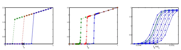
As well as the discrete solution one desires to find, parasitic solutions of the discrete system frequently appear. These may look like solutions of (1.1) but are in fact inaccurate. Figure 2.3 shows some of the phenomena one can encounter. In it, the leftmost diagram shows 3 different solutions computed on the same equidistant mesh. The central diagram, which exhibits solutions computed on 3 different Shishkin meshes, implies that, if one starts from a parasitic solution on a uniform mesh and then uses adaptive mesh refinement, one can converge to a very inaccurate yet plausible computed solution on an adapted mesh. The rightmost diagram reveals a further unpleasant property: for a single Shishkin mesh that is centred ont0, one can compute
multiple discrete solutions each of whose transition layer profiles is shifted by O(ε). The accuracy of such a shifted solution is onlyO(1) in the maximum norm.
Alarmingly, every computed solution in Figure 2.3 looks plausible if one has no precise a priori knowledge of the true location of the interior layer. Consequently any one of these solutions might lead the experimentalist to believe that an interior-layer solution of Example 2.1 has been successfully computed—when in fact the discrete solution is onlyO(1) accurate in the discrete maximum norm.
The inaccuracy of solutions computed on correctly-placed Shishkin meshes in the rightmost diagram of Figure 2.3 will surprise those who view these meshes as a panacea for the computation of layers in the solutions of differential equations. Heuristically, the displacement of the interior layer in solutions of the standard scheme occurs since the discretization of the differential equation may disrupt the mechanism that implicitly puts the interior layer in the correct location. In particular,this mechanism is entirely lost on the coarse mesh whenε≪N−1, as there one is essentially solving
0 1 0
0.5 1 1.5 2 2.5
t
0
0 1
0 0.5 1 1.5 2 2.5
t 0
0.3746 0.3751 0
0.5 1 1.5 2
[image:4.595.79.435.88.187.2]t0+εt1
Fig. 2.3.Parasitic computed solutions of Example 2.1 generated by the standard scheme(4.2)
(different solutions of the same discrete problem are obtained using different initial guesses of type y = 1 + sgn(x−x∗) with variousx∗). Left: equidistant mesh with ε= 0.01, N = 20. Centre: solutions computed on Shishkin meshes centred at three different points with ε = 0.01, N = 40. Right: enlarged multiple solutions of the discrete problem with ε= 10−4,N = 64, on a Shishkin
mesh centred correctly at the point t0 that is defined in (A5); the quantityt1 is defined in [11,
Lemma 2.4]; the mesh transition parameter is specified by (4.4) with Cτ = 4.2. These computed
solutions are obtained using shooting to determine the value ofuNmwherexm=t0+O(ε); the exact
solution is the bold curve.
stabilised scheme cures entirely the instabilities of both Figure 2.1 (see Figure 2.2) and Figure 2.3(left), but in some cases one may still observe the multiple-solution phenomenon of Figure 2.3(centre, right).
Nevertheless, as our theoretical conclusions and numerical results show, when the Shishkin mesh is placed correctly there is then a qualitatively correct discrete solution that isε-uniformly accurate outside the layer region. Furthermore, our Theorem 5.1 gives a range of valuesN that ensureε-uniform convergence in the entire domain and for which we have not observed the multiple-solution phenomenon of Figure 2.3(right).
3. Hypotheses on the data of the continuous problem. In this section we place hypotheses on the data of (1.1). Assume that the reduced problem (1.2) has three simple rootsφ=φk ∈C∞[0,1] for k= 0,1,2:
(A1) b(x, φk(x)) = 0 for k= 0,1,2 and x∈[0,1]
where
(A2)
{
φ1(x)< φ0(x)< φ2(x) forx∈[0,1]
and there is no other solution of (1.2) between φ1 andφ2.
Here and subsequently, numbering such as (A1) indicates anassumption that holds true throughout the paper. Assume also that
(A3) bu(x, φk(x))> γ2>0 for k= 1,2 and x∈[0,1]
but
(A4) bu(x, φ0)<0 for x∈[0,1].
Assumption (A3) says thatφ1(x) andφ2(x) are stable reduced solutions, i.e., one
may have a solutionuof (1.1) that is very close to eitherφ1orφ2on some subdomain
of (0,1). Assumption (A4) means that the solutionφ0(x) is unstable: no solution of
(1.1) lies close to φ0 on any subdomain of (0,1). Under the hypotheses (A1)–(A4),
Our further assumption is that the equation∫φ2(x)
φ1(x) b(x, v)dv= 0 has a solution
x=t0 such that dxd
[ ∫φ2(x)
φ1(x)b(x, v)dv]x=t0 ̸= 0, i.e., this root is simple. As in many
asymptotic analysis papers, we also assume that the value of this derivative is negative, since this sign corresponds to the Lyapunov stability of an interior-layer solutionu(x) of (1.1) that switches from φ1 to φ2 when u is regarded as a steady-state solution
of the time-dependent parabolic problemvt−ε2vxx+b(x, v) = 0 (see [1, Section 7,
Remark 3]; if instead the derivative were positive, this would correspond to Lyapunov stability of an interior-layer solution that switches fromφ2 to φ1). By Assumption
(A1) these hypotheses on the integrals ofbare equivalent to the assumptions
(A5)
∫ φ2(t0)
φ1(t0)
b(t0, v)dv= 0 and
∫ φ2(t0)
φ1(t0)
bx(t0, v)dv=−CI <0.
Similar conditions are assumed in [19,§4.15.4], [20, §2.3.2] and also in [2, 15] for an analogous two-dimensional problem and [4] for a analogous system of equations.
Remark 3.1. Assumption (A2) can be relaxed to allow other roots of (1.2) between φ1 and φ2 provided that
∫v
φ1(t0)b(t0, s)ds > 0 for all v ∈ (φ1(t0), φ2(t0)).
Note that this inequality follows immediately from(A1)–(A5)ifφ0 is the only reduced solution betweenφ1 andφ2.
The solutionsφ1andφ2 of (1.2) do not in general satisfy either of the boundary
conditions in (1.1b). In order to focus on interior layers, we exclude boundary layers by assuming that
(A6) φ1(0) =g0, φ2(1) =g1, φ′′1(0) =φ′′2(1) = 0.
Under Assumptions (A1)–(A6), the problem (1.1) has a solution that, roughly speaking, lies in the neighbourhood ofφ1(x) andφ2(x) forx∈[0, t0) and x∈(t0,1]
respectively (see Corollary 6.7). Near x = t0 the solution switches from φ1 to φ2,
which results in an interior transition layer of widthO(ε|lnε|).
4. Standard and stabilised numerical methods, Shishkin mesh. Here we define our standard and stabilised finite difference methods, and a Shishkin mesh [13, 17, 18] that is tailored to (1.1).
Let N, the number of mesh intervals, be a positive integer. Let the mesh be 0 = x0 < x1 <· · · < xN−1 < xN = 1. Set hi = xi−xi−1 for i = 1, . . . , N, and
~i = (hi+hi+1)/2 for i= 1, . . . , N−1. Throughout the rest of the paper we shall
always assume that
(4.1) ε≤CN−1
for some positive constantC. This assumption is reasonable in practical situations: if it were not satisfied then one could apply standard numerical methods to solve (1.1).
A discrete solution of (1.1) on the mesh will be written as {uN
i } or {uˆNi } for
i= 0,1, . . . , N. The classical finite difference approximations ofu′(xi−1/2) andu′′(xi)
are defined by
DuNi :=u
N
i −uNi−1
hi
, δx2uNi :=Du
N
i+1−DuNi
~i
.
Thestandard finite difference scheme for approximating (1.1) is
FNuNi :=−ε2δx2uNi +b(xi, uNi ) = 0 fori= 1, . . . , N−1,
subject to uN
0 = g0 and uNN = g1. This scheme is also generated by the standard
mass-lumped piecewise linear finite element method. As it frequently produces unsat-isfactory computed solutions—see Section 2—we propose astabilised finite difference scheme
ˆ
FNuˆNi :=−εˆ
2
i+1DˆuNi+1−εˆ2iDuˆNi ~i
+b(xi,uˆiN) = 0 fori= 1, . . . , N−1,
(4.3)
subject to uN
0 = g0 and uNN = g1, where ˆεi := max{ε,Chˆ i} for some user-chosen
positive constant ˆC. Compared with (4.2), we observe that ifhi >Cˆ−1εthen (4.3)
adds artificial diffusion. The stabilised scheme (4.3) can also be generated by a mass-lumped piecewise linear finite element method with artificial diffusion added in a conservative way; in this framework it is easy to generalise (4.3) to higher-dimensional problems.
We now define a Shishkin meshthat is appropriate for (1.1). Define the mesh transition point parameterτ by
(4.4) τ =Cτ
¯
γ εlnN,
where
(4.5) γ¯:=
√
min
k=1,2bu(t0, φk(t0))
(so ¯γ > γ >0,whereγappeared in (A3)) andCτ is a user-chosen constant that should
be sufficiently large—see Theorems 5.1 and 5.2. Assume that εis so small that 1
2t0< t0−τ andt0+τ <1− 1
2(1−t0). Divide
the intervals [0, t0−τ], [t0−τ, t0+τ] and [t0+τ,1] intoN0, N/2 andN1equidistant
subintervals respectively withN0+N1=N/2 andN0≈t0N/2,N1≈(1−t0)N/2. In
practice one usually hasτ ≪1, so the mesh is relatively fine on [t0−τ, t0+τ]. Write hfor this fine mesh width; thenh=CεN−1lnN. On the remainder of [0,1] one has
a coarse mesh of widthO(N−1).
To solve (1.1) numerically one could use a graded mesh, but we shall confine our attention to the piecewise-equidistant Shishkin mesh as it is easier to analyse; cf. [17].
Remark 4.1. Let N be sufficiently large. Then on the above Shishkin mesh, for the discrete operatorsFN andFˆN of (4.2) and (4.3) we haveFˆN =FN if|x
i−t0|< τ. Furthermore,FˆN−FN =−(ˆε2
1−ε2)δ2xifxi< t0−τ, andFˆN−FN =−(ˆε2N−ε2)δx2
if xi> t0+τ.
5. Existence and accuracy of discrete solutions. Main results. This section states existence results for discrete solutions of the standard difference scheme (4.2) and the stabilised scheme (4.3) near an interior-layer solution u of (1.1). The theorems below deal with two regimes that depend on the relative sizes ofεandN.
Theorem 5.1. Let {xi} be the Shishkin mesh of Section 4 that is defined
us-ing (4.4) and (4.5). Set C′ = 4Cτ/γ¯. For some σ ∈ [0,2], assume that c0ε ≥
(C′N−1lnN)2+σ; this constant c
0 is used in Lemma 6.10. Letεbe sufficiently small andN sufficiently large.
(i) If Cτ>2, then there exists a solution uNi of the standard scheme (4.2) such that
(5.1) |uNi −u(xi)| ≤C
{
(N−1lnN)2−σ for |x
i−t0|< τ, N−2 for |x
(ii) IfCτ >3, then there exists a solutionuˆNi of the stabilised scheme (4.3) such that
(5.2) |uˆNi −u(xi)| ≤C
{
(N−1lnN)2−σ+N−1 for |x
i−t0|< τ,
N−1 for |x
i−t0| ≥τ.
The next result considers the possibility that the relationship between εand N
is stronger than (4.1). Fixλ∈(0,1). The caseε≥CN−(4−λ)≥c−1
0 (C′N−1lnN)4
was considered in Theorem 5.1 so now we focus onε≤CN−(4−λ).
Theorem 5.2. Let {xi} be the Shishkin mesh of Section 4 that is defined using
(4.4) and (4.5). Fix λ ∈ (0,1). Assume that ε ≤ CN−θ for some θ ≥ 4−λ and C >0, andN is sufficiently large independently ofε.
(i) If Cτ>2, then there exists a solution uNi of the standard scheme (4.2) such that
(5.3) |uNi −u(xi)| ≤CN−min{2,θ−2}≤CN−(2−λ) for |xi−t0| ≥τ.
(ii) IfCτ >1, then there exists a solutionuˆNi of the stabilised scheme (4.3) such that
(5.4) |uˆNi −u(xi)| ≤CN−1 for |xi−t0| ≥τ.
Remark 5.3. Consider the use of Newton’s method to compute a solution of the standard scheme (4.2). Although Theorems 5.1 and 5.2 guarantee existence of a solution that attains a higher order of convergence, parasitic solutions are numerous and an unsophisticated initial guess in Newton’s method will yield an unsatisfactory result (see Section 2). To obtain a higher-order-accurate solution one should use as initial guess a solution of the stabilised scheme (4.3); see Tables 7.3 and 7.4 below.
Remark 5.4. An inspection of the proof of Theorem 5.1 shows that one still ob-tains existence of a discrete solution satisfying the error estimate (5.1) if the alterna-tive stabilised scheme−max{ε,Cˆ~i}2δx2uNi +b(xi, uNi ) = 0is used. On an equidistant
mesh this scheme is identical with (4.3), while on our Shishkin mesh it differs from (4.3) only at the two transition points t0 ±τ. This alternative stabilisation seems somewhat superior to the standard scheme (4.2), but on our Shishkin mesh, some initial guesses in Newton’s method produce computed solutions having interior layers outside the interval [t0−τ, t0+τ].
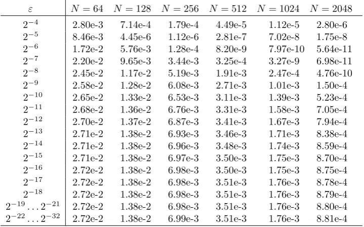
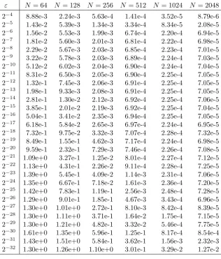
Remark 5.5 (ε-uniform accuracy in the layer region via postprocessing). The-orems 5.1 and 5.2, and the numerical results of Section 7, suggest that as ε→0 for any fixedN, the accuracy of discrete solutions of (4.2)or (4.3)deteriorates inside the layer region{xi :|xi−t0|< τ}. To obtain ε-uniform accuracy in the entire domain
[0,1]for all ε≤CN−1, one can use a postprocessing technique for smaller values of εas follows.
Setε¯:=N−2ln3
N (orε¯:=CN−2ln3
N for any positive constantC), and denote by u¯ the corresponding exact solution of (1.1). Note that ε¯satisfies, for sufficiently large N, the hypothesis of Theorem 5.1 with σ = 0. Consequently, if {u¯Ni } is the computed solution obtained as in part (i) or part (ii) of Theorem 5.1 on the mesh denoted by{x¯i}with the transition parameterτ(¯ε) :=Cγ¯τ ε¯lnN, thenmaxi|u¯iN−u¯(¯xi)|
is bounded, respectively, by CN−2ln2N or CN−1.
Postprocessing forε∈(0,ε¯): For |x¯i−t0| > τ(¯ε), set x˜i := ¯xi and u˜Ni := ¯u N
i ;
for |x¯i−t0| ≤ τ(¯ε), set x˜i :=t0+ ε(¯xiε¯−t0) and u˜Ni := ¯uNi (i.e., in the layer region
the computed solution {u¯N
i } is translated and compressed horizontally). Then the
post-processed solution {u˜Ni } on the mesh{x˜i} satisfies the error estimate
(5.5) max
i |u˜
N
i −u(˜xi)| ≤CN−2ln4N+ max
j |u¯
N
To prove this, it suffices to show that |u¯(¯xi)−u(˜xi)| ≤ CN−2ln4N for all i. Note
that [11, Lemma 2.5], combined with Corollary 6.7 below, implies that|u(x)− U(x, ε)|
and |u¯(x)− U(x,ε¯)| are both bounded by C(¯εlnN +N−2)≤CN−2ln4
N. Here the function U, which is related to the asymptotic expansion uas of (6.3), is defined by
U(x, ε) :=V0(x−εt0; 0)for|x−t0| ≤τ(ε), and U(x, ε) :=u0(x)for|x−t0|> τ(ε). As
U(¯xi,ε¯) =U(˜xi, ε), the required bound for |u¯(¯xi)−u(˜xi)|, and so (5.5) follow.
6. Analysis of the numerical methods. Proof of Theorems 5.1 and 5.2. Section 6 is devoted to the proofs of Theorems 5.1 and 5.2, i.e., here we establish the existence and accuracy of discrete solutions for problem (1.1). Our analysis is based on the use of sub-solutions and super-solutions for the discrete problems (4.2) and (4.3). While Nefedov [15] discusses continuous sub- and super-solutions for a two-dimensional analogue of problem (1.1), the investigation of discrete sub- and super-solutions is more complicated since one must deal not only withεbut also with the other small parameterN−1.
Throughout this section, let{xi}be the Shishkin mesh of Section 4 that is defined
using (4.4) and (4.5). We start by describing briefly asymptotic expansions of that solution of (1.1) that we wish to compute numerically. The expansion of Section 6.1 resembles previously published work [15, 20] so most of the details are diverted to our report [11, Section 2]. In Section 6.2 extra terms are added to this expansion to get sub- and super-solutions of the numerical methods for (1.1). Then in Section 6.3 we estimate the truncation errors of our schemes; these estimates are used in Section 6.4 to establish sufficient conditions for discrete sub- and super-solutions derived from the construction of Section 6.2. Finally, the existence and error estimates of Theorems 5.1 and 5.2—the main results of the paper—are proved in Section 6.5.
6.1. Sketch of asymptotic expansion for the continuous problem. Recall the point t0 ∈ (0,1) that was specified in Assumption (A5). Define the stretched
variableξby
ξ:= (x−t0)/ε.
Then a standard calculation shows that the zero-order interior-layer termV0(ξ) of the
asymptotic expansion ofuis given by a solution of the following problem:
(6.1a) −dξd22V0+b(t0, V0) = 0 forξ∈R, V0(−∞) =φ1(t0), V0(∞) =φ2(t0).
We shall see shortly that (6.1a) has a solution V0(ξ), but this solution is not
unique as V0(ξ±C) is also a solution for any constant C. Once we know that V0
exists and is a strictly increasing function, consider a specific solution ˆV0 of (6.1a)
subject to the parametrization
(6.1b) Vˆ0(0) =φ2(t0).
One might expect u(x) = φ0(t0) to hold at x = t0 and thus the interior layer to
be described by ˆV0(ξ). This is not the case, however; in fact u(x) = φ(t0) when x=t0+εt1+ε2t2+· · ·, and the interior layer is described by ˆV0(ξ−t1−εt2−· · ·). Here t1, t2, . . . are independent of ε and can be found when constructing an asymptotic
expansion of u; in particular, the values of t1 and t2 are specified in the proof of
Lemma 6.3 that appears in [11].
In our analysis we taket=t0+εt1+ε2t2, omitting the higher-order terms, and
invoke a perturbed version of ˆV0(ξ−t1−εt2) defined by
Here the real-valued parameterpsatisfies|p| ≤p∗ for any fixed positive constantp∗, but will typically take very small values.
Lemma 6.1. For any constant¯t1and all|p| ≤p∗, there exists a unique monotone solution V0(ξ;p)of (6.1). Furthermore,V0 is inC∞(R), and
(6.2) χ(ξ;p) := dξdV0(ξ;p)>0 forξ∈R.
For any arbitrarily small but fixedλ∈(0,γ¯), there is a constantCλsuch thatχ(ξ;p)≤
Cλe−(¯γ−λ)|ξ| for ξ ∈ R, |p| ≤p∗. There are constants C′ and C′′ such that for all
|p| ≤p∗ one hasC′χ≤V0−φ1(t0)≤C′′χ for ξ <0 andC′χ≤φ2(t0)−V0≤C′′χ forξ >0.
Proof. In view of (A1)–(A5), these properties follow from the proof of [3, Lemma 2.1] or a slight extension of the proof of [10, Lemma 2.1] using phase-plane analysis.
One then continues the asymptotic analysis of (1.1) along the lines of [20, Section 2.3.2] and [15, Section 3], but with the modification that one expands about the point t0 instead of about the point t = t0+εt1+ε2t2+· · · (which is unknown a
priori); this will aid the numerical analysis because our layer-adapted mesh will be centred on the known point t0. Details of this asymptotic construction are given
in [11, Section 2]. Essentially, two asymptotic expansions are constructed separately on [0, t0] and [t0,1−t0] and then matched at x = t0. One arrives finally at the
expansion
(6.3) uas(x;p) :=u0(x) +ε2u2(x) +v0(ξ;p) +εv1(ξ;p) +ε2v2(ξ;p),
where the smooth componentu0+ε2u2 combines the functions
u0(x) :=
{
φ1(x), x∈[0, t0), φ2(x), x∈(t0,1],
, u2(x) :=u′′0(x)/bu(x, u0(x)),
while the boundary-layer component, whose properties will be described in a moment, isv0+εv1+ε2v2. We use the auxiliary functions
B(x, s) :=b(x, u0(x) +s) and ˆt0= ˆt0(x) :=
{
t−0 ifx∈[0, t0) t+0 ifx∈(t0,1]
(thus for exampleu0(ˆt0) =φ1(t0) forx < t0). Nowv0(ξ) =v0(ξ;p) is defined by
(6.4) −dξd22v0+B(ˆt0, v0) = 0, v0(0±) =V0(0;p)−u0(t±0), v0(±∞) = 0.
Comparing this with (6.1a), we see that
v0(ξ;p) =V0(ξ;p)−u0(ˆt0).
Higher-order interior-layer componentsvj(ξ) =v1(ξ;p) forj= 1,2 are defined by
(6.5) [−dξd22 +Bs(ˆt0, v0)]vj=ψj(ξ), v1(0) =vj(±∞) = 0, v2(0±) =−u2(t±0),
whereψ1(ξ) :=−ξBx(ˆt0, v0), whileψ2is similar, but has a more complicated structure
that is described in [11, (2.13)]. The functions v1 and v2 depend on p since they
u0+v0= [u0(x)−u0(ˆt0)] +V0 and u2+v2are continuous at x=t0. Thusuas(x;p)
is continuous forx∈[0,1].
Lemma 6.2. For any constants t1 andt2 in (6.1c), there exist solutions v0, v1 andv2 of the problems (6.4), (6.5). The functionv0 satisfies
(6.6) (sgnξ)·v0(ξ)>0 and |v0(ξ)| ≤C′′χ(ξ) forξ∈R\ {0}.
Furthermore, assuming that|t1|+|t2| ≤C and|p| ≤p∗, for any arbitrarily small but fixedλ∈(0,γ¯), there is a constantCλ such that
(6.7) dk
dξkvj≤Cλe−(¯γ−λ)|ξ| for ξ∈R\ {0}, j= 0,1,2, k= 0, . . . ,6.
Proof. We outline the proof; for details see [11, Lemma 2.3]. First, Lemma 6.1 yields existence of the function v0, the properties (6.6), and the bound (6.7) for j = 0, k = 0,1. The remaining assertions are derived on noting that v1, v2 and
dk
dξkvj, for j = 0,1,2, all satisfy linear differential equations that share the same
operator [−d2
dξ2+Bs(ˆt0, v0)] —one can then use an explicit solution formula obtained
by variation of parameters since the functionχof (6.2) satisfies [−dξd22+Bs(ˆt0, v0)]χ=
0; see [3, Lemma 2.2].
Given any suitable functionv(x), define the functional
Φ[v(·)] :=εdvdxx=t−
0 −
εdvdxx=t+ 0
.
The main result of this section now follows.
Lemma 6.3. For the asymptotic expansion uas(x;p) from (6.3) we have
(6.8a) F uas(x;p) =O(ε3) forx∈(0,1)\ {t0}.
Furthermore, there exist values of t1 and t2 in (6.1c), independent of ε and p, and positive constants C1,C2 andε∗ =ε∗(p∗) such that for allε≤ε∗ and0 <|p| ≤p∗ we have
(6.8b) (sgnp)·Φ[uas(·;p)]≥C1ε|p| −C2ε3.
Proof. We sketch the detailed proof that is given in [11, Lemma 2.4]: the relation (6.8a) is a standard outcome of the method of asymptotic expansions that was applied to generate the terms in (6.3), while to establish (6.8b) one uses Φ[u0] =ε[φ′1(t0)− φ′2(t0)], Φ[v0] = Φ[V0] = 0, Φ[ε2u2] = O(ε3), and Φ[εv1+ε2v2] is computed using
explicit representations ofv1andv2described in the proof of Lemma 6.2.
Note that Lemma 6.3 implies that there exists|p0| ≤ε2CC2
1 such thatuas(x;p0)∈
C2[0,1] soF u
as(x;p0) =O(ε3) for allx∈(0,1), which is a standard property of an
asymptotic expansion.
6.2. Perturbed asymptotic expansion, sub- and super-solutions. For the numerical analysis that comes later, we modify the asymptotic expansionuas(x;p) of
(6.3): set
The functionβis a small perturbation ofuaswhen the parametersp′ and ˆhare small.
The parameter ˆhis related to the mesh used and the component ˆh2z(ξ;p) is added
to compensate for the principal part of the truncation error produced when our finite difference operator is applied to uas(x, t). The component p′[v∗(ξ;p) +C0] is added
to ensure that (sgnp′)·F(uas+p′[v∗+C0])≥0.
The functionsv∗(ξ) =v∗(ξ;p) andz(ξ) =z(ξ;p) used in (6.9) are defined by
[−d2
dξ2 +Bs(ˆt0, v0)]v∗=|v0| forξ∈R\ {0}, v∗(0) =v∗(±∞) = 0,
(6.10)
[−dξd22 +Bs(ˆt0, v0)]z = 121 d
4
dξ4V0 forξ∈R, z(0) =z(±∞) = 0.
(6.11)
These functions depend onpsince they are defined usingv0(ξ;p) andV0(ξ;p). Lemma 6.4. Assume that|p| ≤p∗for some positive constantp∗. Then there exist solutions v∗ andz of problems (6.10) and (6.11) respectively, and for any arbitrarily small but fixedλ∈(0,γ¯), there is a constantCλ such that
(6.12) v∗≥0, dξdkkv∗+ dk
dξkz≤Cλe−(¯γ−λ)|ξ| for ξ∈R\ {0}, k= 0, . . . ,4.
Furthermore, there exist positive constantsC1,C2,C3 andε∗ =ε∗(p∗)such that for allε≤ε∗ and0<|p| ≤p∗ we have
(6.13) (sgnp)·Φ[β(x;p, p′,ˆh)]≥C1ε|p| −C2ε3−C3|p′|.
Proof. A detailed proof is given in [11, Lemma 3.1]. In this, like the proof of Lemma 6.2, we use explicit solution formulas for v∗ and z that are derived from a particular solution χ of the corresponding homogeneous equation. One thereby obtains Φ[v∗]≥ −C3 and the crucial identity Φ[z] =−χ(0)1
∫∞
−∞(121
d4
dξ4V0)χ dξ= 0.
Lemma 6.5. There exist positive constantsC0,C4,p′∗ and ε∗ such that for all x∈(0,1)\ {t0},ε≤ε∗,|p| ≤p∗,0<|p′| ≤p′∗, the function β of (6.9) satisfies
(6.14) (sgnp′)·[F β−12ˆh2dξd44V0]≥12C0|p′|γ2−C4(ε3+εˆh2+ ˆh4).
Proof. Imitate the analysis of [10, Lemma 3.2]; for details see [11, Lemma 3.2].
Lemma 6.6. Let p≥0, p′ =C′εp for some positive constant C′, and ˆh2≤Cεµ for some fixedµ∈(0,1]. Then there exists ε∗=ε∗(C′, µ) such that for the function β from (6.9) we have
(6.15) β(x;−p,−p′,ˆh)≤β(x;p, p′,ˆh) for x∈[0,1], ε≤ε∗, |p| ≤p∗.
Furthermore, for any arbitrarily small but fixedλ∈(0,γ¯), there is a constantCλ such
that uas from (6.3) satisfies
(6.16) |β(x;±p,±p′,hˆ)−uas(x; 0)| ≤Cλ(|p|+ ˆh2)e−(¯γ−λ)|ξ|+Cε|p|.
Proof. This result is obtained using the exponential decay of ∂
∂pv0=χ >0 and ∂
∂pvj, ∂
∂pv∗
∂
∂pz; see [11, Lemma 3.3] for further details.
Corollary 6.7. There isε∗>0 such that for allε≤ε∗ there exists a solution uof problem (1.1) that satisfies
(6.17) |u(x)−uas(x; 0)| ≤Cε2 for x∈[0,1].
Proof. Let ¯p ≥ C2ε2/(2C1) and ¯p′ = C1εp/¯ (2C3). By (6.13) we then get
±Φ[β(·;±p,¯ ±p¯′,0)] ≥ 0. Choose ¯p = O(ε2) so large that 12C0p¯′γ2 ≥ C4ε3; then
by (6.14) one obtains ±F β(x;±p,¯ ±p¯′,0) ≥0 for x∈ [0,1]\ {t0}. Furthermore, by
(6.15), we have β(x;−p,¯ −p¯′,0) ≤ β(x; ¯p,p¯′,0) for x ∈ [0,1]. Thus β(x;−p,¯ −p¯′,0) andβ(x; ¯p,p¯′,0) are ordered sub- and super-solutions for the equation (1.1a). In view of (A6), one gets±β(x;±p,¯ ±p¯′,0)x=0,1 ≥g0,1, soβ(x;−p,¯ −p¯′,0) and β(x; ¯p,p¯′,0)
are sub- and super-solutions for the entire problem (1.1). It follows [16, Corollary 7.1 of Chapter 1] that there exists a solutionuof (1.1) that lies between these sub- and super-solutions. By (6.16), this solution lies in an O(¯p) = O(ε2) neighbourhood of uas(x; 0).
A similar result can be found in [15] but for a slightly different asymptotic ex-pansion.
6.3. Truncation error. We first examine the truncation error of the discrete operatorsFN and ˆFN of (4.2) and (4.3) applied on our Shishkin mesh to a particular
case ofβ from (6.9). Set
(6.18) β∗(x) =β∗(x;p) =β(x;p, p′,ˆh), where ˆh:=h/ε=CN−1lnN, p′ :=εC1
2C3 p,
wherepis such that|p| ≤p∗ for some fixed positive constantp∗, and
(6.19) Ii:=
{
1 for |xi−t0| ≥τ,
0 for |xi−t0|< τ.
Lemma 6.8. Let Cτ>2. Fix pwith |p| ≤p∗. Then
(6.20a) FNβ∗(xi)−F β∗(xi) =−
ˆ
h2
12
d4
dξ4V0(ξi) +O(εˆh2+ ˆh4+N−2Ii) forxi ̸=t0,
whereξi= (xi−t0)/ε, and
(6.20b) FNβ∗(t0)−12[F β∗(t−0)+F β∗(t + 0)] =−
ˆ
h2
12
d4
dξ4V0(0)+ˆh−1
{
Φ[β]+O(εˆh2+ˆh4)}.
Furthermore,
(6.20c) |( ˆFN −FN)β∗(xi)| ≤CN−1Ii.
Proof. Throughout this proof we writeβ forβ∗. (a) ClearlyFNv
i−F v(xi) =−ε2[δx2vi−d
2
dx2v(xi)] =:ri[v] for any suitable function
v(x). Thus we need to estimate ri[β]. Let xi ̸= t0. First, one has |r[u0+ε2u2]| ≤ Cε2N−1 ≤Cεhˆ2, where we used (4.1). In the exponential-decay estimates (6.7) and (6.12), chooseλsufficiently small so thatCτ(1−λ/¯γ)≥2 and thuse−(¯γ−λ)τ /ε≤N−2
noting that (6.18) implies |p′| ≤Cε, we now have |r[β−v0]| ≤C(ε+p′+ ˆh2)ˆh2 ≤ C(εˆh2+ ˆh4), so we will be done if we show that
(6.21) ri[v0] =ri[V0] =− ˆ
h2
12
d4
dξ4V0(ξi) +O(ˆh4+N−2Ii).
For all|xi−t0|< τ, the relationship (6.21) follows from a standard truncation error
analysis using ε2h122dxd44V0 = ˆ
h2
12
d4
dξ4V0 and ε2h4d
6
dx6V0 = ˆh4d
6
dξ6V0 = O(ˆh4); while if
|xi−t0| ≥τ, then by (6.7) the above choice ofλyields|r[v0]| ≤2ε2|d
2
dx2v0| ≤CN−2≤
Cˆh2 and ˆh2
12
d4
dξ4V0(ξi) ≤Cˆh2N−2 ≤Cˆh4, so we again get (6.21). Thus (6.20a) is
established.
(b) Atxi =t0, one again has (6.21) and it remains to estimate the truncation
errorr[ ˜β] for the function ˜β(x) :=β(x)−V0(ξ). This function is continuous but has
a discontinuous derivative atx=t0. Note that
(6.22) β˜(t0±h) = ˜β(t0)±hdxd β˜(t±0) +
h2
2
d2
dx2β˜(t±0)±
h3
6
d3 dx3β˜(ˆx±)
for some|xˆ±−t0| ≤h. Now d
3
dx3β˜=
d3
dx3[u0+ε2u2] +ε−3d
3
dξ3[εv1+ε2v2+p′v∗+ ˆh2z],
so|dxd33β˜| ≤Cε−
3(ε+p′+ ˆh2)≤Cε−3(ε+ ˆh2). A calculation using (6.22) gives
−ε2δx2β˜
t0=
ε
hΦ[ ˜β]−
1 2ε
2[d2
dx2β˜(t−0) +
d2 dx2β˜(t
+
0)] + ˆh O(ε+ ˆh 2).
Combining this with (6.21) at xi = t0, where ξi = 0, and noting thatε/h = ˆh−1,
Φ[ ˜β] = Φ[β], and dxd22V0 is continuous atx=t0, we get
−ε2δ2xβt0 = ˆh−1Φ[β]−12ε 2[d2
dx2β(t−0) +
d2
dx2β(t
+ 0)]−
ˆ
h2
12
d4
dξ4V0(0) + ˆh−1O(εˆh2+ ˆh4),
which yields (6.20b).
(c) Combining Remark 4.1 with the observations that ˆε2
i ≤CN−2and|δ2xβ| ≤C
for|xi−t0|> τ, we immediately get|( ˆFN −FN)β(xi)| ≤CN−2Ii for|xi−t0| ̸=τ.
Now letxn=t0−τ so|( ˆFN −FN)β(xn)| ≤~−n1(ˆε2n−ε2)|Dβ(xn)| ≤CN−1, where
we used~−1
n ≤CN, ˆε2n−ε2≤CN−2 and|Dβ(xn)| ≤C. Getting a similar bound at
xi=t0+τ completes the proof of (6.20c).
To deal with the termsN−2I
i andN−1Iiin the above truncation error estimates,
we need the following lemma.
Lemma 6.9. Let N be sufficiently large and p′′ > 0 be sufficiently small, in-dependently of ε. Let Cτ′ < Cτ. Then there exists wi such that 0 ≤ wi ≤ 1 and
for all |p| ≤p∗ the functionβ∗(x;p) from (6.18) satisfies ±{FN[β
∗(xi;p)±p′′wi]−
FNβ
∗(xi;p)} ≥p′′(γ2Ii−CN−C ′
τ). Furthermore, this estimate holds true with FN
replaced byFˆN.
Proof. Chooseλsufficiently small so thatCτ(1−λ/γ¯)≥Cτ′. We claim that there
are a sufficiently smallc′ and a sufficiently large ¯C′ such that for all|p| ≤p∗we have
(6.23) bu(x, β∗(x) +s)≥
{
γ2 for εC¯′ ≤ |x−t0|, |s| ≤c′, (¯γ−λ/2)2 for εC¯′ ≤ |x−t0|< τ, |s| ≤c′.
Indeed, forx < t0(the other case is similar), one hasbu(x, β∗(x) +s) =bu(x, φ1(x)) + O(β∗−φ1)+O(s), where the termO(s) can be made as small as needed by choosingc′
sufficiently small, while β∗(x) = φ1(x) +v0+O(N−1) so the termO(β∗−φ1) can
observation with Assumption (A3) for bu(x, φ1(x)) yields the first bound of (6.23).
Next, forεC¯′ ≤t0−x < τ, one hasbu(x, φ1(x)) =bu(t0, φ1(t0))+O(τ)≥¯γ2−CεlnN
by (4.5), so by virtue of (4.1) we get the second bound of (6.23) for sufficiently large
N. Define
wi:=
{
1 for |xi−t0| ≥τ, ω(xi)e−(¯γ−λ)(τ−|xi−t0|)/ε for |xi−t0|< τ,
whereω(x) is a smooth cut-off function that takes values in [0,1], equals 1 for|x−t0| ≥
2εC¯′ and vanishes for |x−t0| ≤εC¯′. As 0≤wi≤1, choosing 0< p′′≤c′, we apply
the standard linearisation and then invoke (6.23) to get
FN[β∗(xi) +p′′wi]−FNβ∗(xi)
≥p′′
−ε2δ2
xwi+γ2wi for τ≤ |xi−t0|,
−ε2δ2
xwi+ (¯γ−λ/2)2wi for εC¯′ ≤ |xi−t0|< τ,
0 for |xi−t0|< εC¯′,
≥p′′
γ2 for|xi−t0| ≥τ,
0 for|xi−t0| ∈[0, τ)\(εC¯′,2εC¯′),
−CN−Cτ′ for|x
i−t0| ∈(εC¯′,2εC¯′).
(6.24)
Here we used −δ2
xwi ≥ 0 for |xi −t0| = τ and ε|dxdω|+ε2| d
2
dx2ω| ≤ C combined
with e−(¯γ−λ)(τ−|x−t0|)/ε ≤ CN−Cτ′ for |x−t0| ∈ (εC¯′−h,2εC¯′+h). (The final
estimate here follows from the choice of λ earlier, which implies that e−(¯γ−λ)τ /ε ≤ N−C′τ.) Now, in view of the definition (6.19) ofIi, (6.24) yields the desired result for
FN[β∗(xi) +p′′wi]−FNβ∗(xi).
The assertions forFN[β
∗(xi)−p′′wi]−FNβ∗(xi) and ˆFN[β∗(xi)±p′′wi]−FˆNβ∗(xi)
are obtained similarly. In particular, when carrying out the analysis for ˆFN, we use Remark 4.1 and the following two observations: δ2xwi = 0 for |xi−t0| > τ and the
stabilised discretization of ε2d2
dx2 in ˆFN, when applied to wi, simply yieldsε2δ2xwi at
|xi−t0|=τ (e.g., at xn =t0−τ we have~n−1[ε2Dwn+1−εˆ2n·0] =ε2δx2wn). Hence
(6.24) withFN replaced by ˆFN remains true.
6.4. Sufficient conditions for discrete sub-solutions and super-solutions. Combining Lemmas 6.8 and 6.9 with the bounds for β that were obtained in Sec-tion 6.2, we now establish sufficient condiSec-tions for β∗(x;±p)±p′′wi to be sub- and
super-solutions of the discrete equations (4.2) and (4.3).
Lemma 6.10. Let Cτ>2. There exist sufficiently large positive constantsC¯,C¯′
and sufficiently small positive constantsε∗=ε∗(p∗),c0=c0(p∗)andc1=c1(p∗)such that if ε≤ε∗,N ≥c1−1 andˆh4≤c
0ε, thenp¯:= ¯C(ε2+ ˆh2+ ˆh4/ε)≤p∗, and β∗(x;p) from (6.18) withp=±p¯satisfies
(6.25) FN[β∗(xi;−p¯)−C¯′N−2wi]≤0≤FN[β∗(xi; ¯p) + ¯C′N−2wi]
fori= 1, . . . , N −1, where0≤wi≤1.
Furthermore, ifCτ >3, then fori= 1, . . . , N−1we have
Proof. By (6.18), sgnp= sgnp′. Combining (6.20a) with (6.14) yields
(6.27a) (sgnp)·FNβ∗(xi;p)≥12C0|p′|γ2−C4′(ε
3+εˆh2+ ˆh4+N−2I
i) forxi̸=t0,
where C4′ > C4 and takes into account the term O(εhˆ2+ ˆh4+N−2Ii) in (6.20a).
Similarly, atxi=t0, using (6.20b) and (6.14), we get
(sgnp)·FNβ∗(t0;p)≥ 12C0|p′|γ2−C4(ε3+εˆh2+ˆh4)+ˆh−1
{
(sgnp)·Φ[β]+O(εhˆ2+ˆh4)}.
Combining this inequality with (6.13)—in which, by (6.18), we have C1εp−C3p′ = 1
2C1εp—we arrive at
(sgnp)·FNβ∗(t0;p)≥12C0|p′|γ2−C4′(ε
3+εˆh2+ ˆh4)
(6.27b)
+1ˆ
h
{1
2C1ε|p| −C2ε 3−
C3′(εhˆ 2
+ ˆh4)}
for some C3′ andC4′ > C4. Applying Lemma 6.9 with p′′ := ¯C′N−2 ≥(C4′/γ2)N−2
andCτ′ := 2< Cτ, one gets
(6.28) ±{FN[β∗(xi)±C¯′N−2wi]−FNβ∗(xi)
}
≥C4′N−2Ii−C5N−4
for someC5>0. The desired assertion (6.25) now follows from (6.27) combined with
(6.28) provided that there exist ¯p∈(0, p∗] and ¯p′ :=εC1
2C3p¯that satisfy
1 2C0p¯′γ
2≥C′ 4(ε
3+εˆh2+ ˆh4) +C
5N−4 and 12C1εp¯≥C2ε3+C3′(εˆh 2+ ˆh4).
AsN−4≤Cˆh2, we choose ¯p:= ¯C(ε2+ˆh2+ˆh4/ε) for some sufficiently large ¯C, and then
impose the conditionsε≤ε∗,N ≥c1−1 and ˆh4≤c0εso that ¯C(ε2+ ˆh2+ ˆh4/ε)≤p∗.
The relation (6.26) is established in a similar manner invoking (6.20c) and choos-ingp′′:= ¯C′N−1 andC′
τ = 3< Cτ in Lemma 6.9.
6.5. Proofs of Theorems 5.1 and 5.2. We are finally ready to establish the main results of the paper.
Proof of Theorem 5.1. (i) First, c0ε ≥hˆ2+σ ≥ˆh4. By Lemma 6.10, we choose
¯
p= ¯C(ε2+ ˆh2+ ˆh4/ε)≤C(N−1lnN)2−σsuch that (6.25) holds true with 0≤w
i≤1.
Furthermore, applying Lemma 6.6 withµ= 1/2 yieldsβ∗(xi;−p¯)≤β∗(xi; ¯p), while
Assumption (A6) implies that±β∗(x;±p¯)x=0,1≥g0,1. These observations imply that β∗(xi;−p¯)−C¯′N−2wi andβ∗(xi; ¯p) + ¯C′N−2wi are ordered sub- and super-solutions
for the discrete problem (4.2). Hence, invoking [10, Lemma 3.1] (see also [12]), we conclude that there exists a solution{uN
i }of (4.2) such thatβ∗(xi;−p¯)−C¯′N−2wi≤
uN
i ≤β∗(xi; ¯p) + ¯C′N−2wi.
But combining (6.16), (6.17) and (4.1) shows that for allione has|β∗(xi;±p¯)−
u(xi)| ≤Cpe¯ −(¯γ−λ)|ξ|+C(εp¯+N−2). It now follows that|uNi −u(xi)| ≤Cpe¯ −(¯γ−λ)|ξ|+
C(εp¯+N−2) for alli. This implies |uN
i −u(xi)| ≤C(¯p+N−2)≤C(N−1lnN)2−σ
for |xi−t0| < τ. For |xi −t0| ≥ τ, by choosing λ as in the proof of Lemma 6.8
one obtains e−(¯γ−λ)|ξ| ≤ N−2 and εp¯ = ¯C(ε3+εˆh2+ ˆh4) ≤ CN−2, which imply |uNi −u(x)| ≤CN−2. Thus we have obtained the error estimate (5.1).
(ii) The existence of ˆuN
i and the error estimate (5.2) are established in a similar
manner, but using β∗(xi;±p¯)±C¯′N−1wi as discrete sub- and super-solutions and
Proof of Theorem 5.2. Here we use simpler sub- and super-solutions based on the function
α(xi;p;I1) :=
{
φ1(xi) +p for i∈ I1,
φ2(xi) +p for i∈ I2={0, . . . , N} \ I1.
(i) Set ¯p:= ¯CN−min{2,θ−2}. We claim that for sufficiently large ¯C, the functions
˜
α = α(xi;−p¯;{xi < t0+τ}) and ˆα = α(xi; ¯p;{xi ≤ t0−τ}) are ordered discrete
sub- and super-solutions for (4.2). Indeed, forxn =t0−τ we have −ε2δ2xαˆn+1 ≥0
and also ε2|δ2
xαˆn| ≤ Cε2~n−1[1 +h−1] ≤ CN−(θ−2) as ~−n1 = O(N) and ε2/h =
ε/hˆ ≤CN−(θ−1). Note also that ε2|δ2
xαˆ| ≤Cε2 ≤CN−2 at the other mesh points.
Combining this with b(x,αˆ) ≥ 1 2γ
2p¯ yields FNαˆ ≥ 0. Similarly, FNα˜ ≤ 0.
Con-sequently there exists a discrete solution {uN
i } of (4.2) such that ˜α ≤ uNi ≤ αˆ
for all i. But as Cτ > 2, for |xi −t0| > τ one gets (writing α for ˜α and ˆα) α = u0(x) +O(¯p) = u(x) +O(ε2 +N−2+ ¯p) = u(x) +O(N−min{2,θ−2}), which
immediately yields (5.3). (ii) The existence of{uˆN
i }and the error estimate (5.4) are established in a similar
manner by showing that ˜αand ˆα, but with ¯p:= ¯CN−1, are discrete sub- and
super-solutions for (4.3). In particular, we use three observations: first, the discretization of ε2dxd22 in ˆF
N applied to ˆα at t
0±τ is bounded by CN−1, e.g., atxn =t0−τ it
is bounded byC~−n1[ε2/h+ ˆε2n]≤CN−1 as ~−n1 =O(N),ε2/h=ε/ˆh≤CN−2 and ˆ
ε2n = O(N−2); second, the same quantity at xn+1 is clearly non-negative; third, in
view of Remark 4.1 and ˆε2
i ≤CN−2, the discretization of ε2 d2
dx2 in ˆFN applied to ˆα
at the other mesh points is bounded byCN−2. Consequently, as in part (i) of the
proof, there exists a discrete solution {uˆN
i } of (4.3) such that ˜α≤uˆNi ≤αˆ for all i.
ButCτ >1 implies thatu0(x) =u(x) +O(ε2+N−1) for|xi−t0|> τ, which leads to
the error estimate (5.4).
Remark 6.11. An inspection of the proof of Theorem 5.2 shows that its statement remains valid on other layer-adapted meshes, such as the Bakhvalov mesh, whose description can be found, e.g., in [8, 9, 17]. But it would be more difficult to establish a version of Theorem 5.1 on layer-adapted meshes other than the Shishkin mesh, because dealing with the principal part of the intricate truncation error estimated in Lemma 6.8 would require an alteration of the statement of this lemma and consequently some modification of the right-hand side in problem (6.11) would be needed.
7. Numerical results. In this section we present numerical results for the interior-layer solution of Example 2.1 displayed in Figure 2.2. It is not feasible to construct a truly representative test problem whose exact solution is known, since the location of the interior layer in such a problem must depend on ε in a very compli-cated way, as the analysis of Section 6.1 reveals. Thus for Example 2.1 we computed reference solutions by using a Shishkin mesh withN = 215(centred aboutt:=t
0+εt1
witht1≈ −1.45 defined in [11, Lemma 2.4]) and combining the standard
discretiza-tion (4.2) on the intervals [0, t] and [t,1] with shooting in the valueUn= 1 +O(ε) at
xn=t.
All our results below are for the Shishkin mesh of Section 4 centred about t0,
with the transition parameterτ := min{(3.25ε/γ¯) ln(N/4), t0/2}. Thus in (4.4) we
have set Cτ := 3.25, replaced lnN by ln(N/4), and also required τ ≤t0/2; all our
theoretical conclusions still remain valid.