Allendes Flores, Alejandro Ignacio and Barrenechea, Gabriel and
Hernández, Erwin and Valentin, Frédéric (2011) A two-level enriched
finite element method for a mixed problem. Mathematics of
Computation, 80. pp. 11-41. ISSN 0025-5718 ,
http://dx.doi.org/10.1090/S0025-5718-2010-02364-6
This version is available at
https://strathprints.strath.ac.uk/29059/
Strathprints is designed to allow users to access the research output of the University of Strathclyde. Unless otherwise explicitly stated on the manuscript, Copyright © and Moral Rights for the papers on this site are retained by the individual authors and/or other copyright owners. Please check the manuscript for details of any other licences that may have been applied. You may not engage in further distribution of the material for any profitmaking activities or any commercial gain. You may freely distribute both the url (https://strathprints.strath.ac.uk/) and the content of this paper for research or private study, educational, or not-for-profit purposes without prior permission or charge.
Any correspondence concerning this service should be sent to the Strathprints administrator:
The Strathprints institutional repository (https://strathprints.strath.ac.uk) is a digital archive of University of Strathclyde research outputs. It has been developed to disseminate open access research outputs, expose data about those outputs, and enable the
MIXED PROBLEM
ALEJANDRO ALLENDES, GABRIEL R. BARRENECHEA, ERWIN HERN ´ANDEZ1
,
AND FR´ED´ERIC VALENTIN2
Abstract. The simplest pair of spacesP1/P0 is made inf-sup stable for the mixed form of
the Darcy equation. The key ingredient is enhance the finite element spaces inside a Petrov-Galerkin framework with functions satisfying element-wise local Darcy problems with right hand sides depending on the residuals over elements and edges. The enriched method is symmetric, locally mass conservative and keeps the degrees of freedom of the original interpolation spaces. First, we assume local enrichments exactly computed and we prove uniqueness and optimal error estimates in natural norms. Then, a low cost two-level finite element method is proposed to effectively obtain enhancing basis functions. The approach lays on a two-scales numerical analysis and shows that well-posedness and optimality is kept despite of the second level numerical approximation. Several numerical experiments validate the theoretical results and compares (favourably in some cases) our results with the classical Raviart-Thomas element.
1. Introduction
The selection of finite dimensional spaces for the Galerkin method demands careful at-tention when it comes to solve the weak form of mixed boundary value problems. In fact, mixed problems can be handled by polynomial interpolations if the pair of spaces fulfill the well-know inf-sup condition [11]. This leads some very popular choices such as equal order interpolations spaces and the simplest elementP1/P0 out of reach, or it prevents nodal values to be chosen as degrees of freedom if some physical properties (such as local conservation of mass) are to be satisfied by the numerical method (cf. [9]).
On the quest to systematically build stable and accurate finite element methods, numeri-cal solutions have been formally decomposed into a solved and an unsolved part with respect to a fixed mesh. Roughly, the resolved part solves the original weak form on a given finite
Date: October 9, 2008.
1
This author is supported by CONICYT Chile, through FONDECYT Project No. 1070276 and by Universidad Santa Mar´ıa through project No. DGIP-USM 120851.
2
This author is supported by CNPq /Brazil Grant No. 304051/2006-3, FAPERJ/Brazil Grant No. E-26/100.519/2007.
element space regardless any numerical drawback, while the unsolved part comes into play to make the complete solution to be free of numerical troubles and recover missed physical properties as well. The final methods are said to incorporate ”missing scales” not captured by the mesh, and so, named multi-scale methods. Different approaches to model the unsolved scales have been proposed over the past years, among which we might mention the Varia-tional Multi-Scale method (VMS) [24] and variations of it [3, 16], the Residual-Free-Bubble approach (RFB) [14, 27, 13] and its practical implementation using a two-level method [22], the Heterogeneous Multi-Scale Methods (HMM) [18], and recently, Petrov-Galerkin Enriched Methods (PGEM) (see [21, 20, 5], and [1] for a survey). Overall, algorithms are closely re-lated by making the unsolved contribution dependent on geometrical aspects of the mesh, the interpolation space choice and the boundary value problem itself. In parallel, RFB and PGEM have been systematically related to stabilized methods and stabilization parameters been obtained with respect the mean value of enriching basis functions [4, 12, 7, 8, 2].
This work addresses the subject for the Darcy equation, a model that appears in porous media, in the Petrov-Galerkin enriched framework. The PGEM has been introduced as a way to incorporate edge residual contribution into the unsolved scale modeling, an aspect neglected by the RFB and responsible for the non-physical oscillations in the numerical solu-tions. In [5] the standard trial and test finite element spaces P1/P0 are differently enriched. The latter remains been enhanced with bubble functions as in the RFB method, but now the trial space incorporates functions driven by the Darcy operator depending on the resid-ual of the equation in each element and on each edge of the triangulation. The boundary conditions for the local problems are set in such a way they ensure the continuity of both the normal component of the enriched velocity (strongly) and pressure (weakly). Thereby, the desired features of the P1/P0 element are preserved, namely its simplicity along with its nodal-valued degrees of freedom for the velocity and the locally mass conservative velocity field.
show the leading error between both methods tends faster to zero than the error itself when the characteristic length of the mesh goes to zero.
Next, the semi discrete method analyzed before is completely discretized using a two-level approach incorporating numerically computed unsolved scales into the enriched method. The order of convergence is not affected by this approximation under mild conditions on the fine scale discretization. It is worth mentioning that, up to our knowledge, few works incorporate fine scales approximation in the numerical analysis. Moreover, a low-cost proce-dure has been proposed to effectively incorporate the subscales. As a matter of fact, as fine scale mesh, one singleP1 element is used throughout all the numerical experiments, keeping optimal convergence. Although not theoretically proved, numerical results highlight qua-dratic convergence for the velocity in theL2 norm, a feature that is clearly not expected for the Raviart-Thomas element [26, 11]. The comparison with the standard Raviart-Thomas method is pushed further and allow us to outline the main features of the two-level enriched method, namely:
• has lower number of degrees of freedom for a fixed mesh;
• induces a symmetric linear system (if we were disposed to relax the symmetry re-quirement, then an equivalent non symmetric but positive definite system may be proposed);
• keeps nodal-valued degrees of freedom for the velocity;
• is locally mass conservative.
The remainder of the paper is as follows: the current section ends with notations and preliminary results; for the sake of completeness the derivation of the PGEM in [5] is revisited in Section 2, and then, the resulting methods are mathematically analyzed in Section 3. Section 4 is devoted to the two-level enriched method which is numerically validated in Section 5. Conclusions are drawn in Section 6.
1.1. Notations. This section introduces definitions and notations used throughout. In what follows, Ω denotes an open bounded domain in R2 with polygonal boundary ∂Ω, and x = (x1, x2) is a typical point in Ω. As usual, L2(Ω) is the space of square integrable functions over Ω,L2
0(Ω) represents functions belonging toL2(Ω) with zero average in Ω, andH(div,Ω)
(H(curl,Ω)) is composed by functions that belong toL2(Ω)2 with divergence (curl) inL2(Ω).
The space H0(div,Ω) stands for the space of functions belonging to H(div,Ω) which have normal component vanishing on∂Ω. Finally, (·,·)D stands for the inner product inL2(D) (or
inL2(D)2, when necessary), andk· k
s,D (|· |s,D) the norm (seminorm) inHs(D) (orHs(D)2),
From now on we denote by {TH} a family of regular triangulations of Ω built up using
triangles K with boundary ∂K composed by edges F. The set of internal edges of the triangulation TH is denoted by EH. The characteristic length of K and F are denoted by
HK and HF, respectively, and H := max{HK : K ∈ TH}, and due to the mesh regularity
there exists a positive constant C such that HF ≤ HK ≤C HF, for all F ⊆ ∂K. Also, for
eachF =K∩K′
∈ EH we choose, once and for all, an unit normal vector nwhich coincides
with the unit outward normal vector when F ⊆ ∂Ω. The standard outward normal vector at the edge F with respect to the element K is denoted by nKF. Moreover, for a function q,
JqK denotes its jump, defined by (see Figure 1):
JqK(x) := lim
δ→0+q(x+δn)−δlim
→0−q(x+δn),
(1)
and JqK= 0 ifF ⊆∂Ω. We finally introduce the following broken spaces:
H0(div,TH) := {v∈L2(Ω)2 : v
K ∈H0(div, K)∀K ∈ TH},
(2)
L20(TH) := {q∈L2(Ω) : q
K ∈L
2
0(K)∀K ∈ TH}.
(3)
n
F
K
K
’Figure 1. The normal vector.
1.2. Preliminaries. In this work we consider the following Darcy problem: Find (u, p) such that
σu+∇p=f, ∇ ·u=g in Ω,
(4)
u·n= 0 on∂Ω,
where σ = µκ ∈ R+ is assumed constant in Ω, with µ and κ denoting the viscosity and permeability, respectively. Here, u is the so-called Darcy velocity, p is the pressure, f and
we assume that the usual compatibility condition Z
Ω
g = 0,
holds.
The standard mixed variational formulation associated with (4) reads: Find (u, p) ∈
H0(div,Ω)×L20(Ω) such that
A((u, p),(v, q)) =L(v, q) ∀(v, q)∈H0(div,Ω)×L20(Ω), (5)
where
A((u, p),(v, q)) := (σu,v)Ω−(p,∇·v)Ω−(q,∇·u)Ω, L(v, q) := (f,v)Ω−(g, q)Ω.
The well-posedness of (5) follows from the classical Babuska-Brezzi theory for variational problems with constraints (see [11] for details).
2. The enriched finite element method
We start generalizing the derivation carried out in [5]. We introduce the standard finite element space VH := [VH]2∩H0(div,Ω) for the velocity variable, where
VH :={v ∈C0 Ω
:v|K ∈P1(K), ∀K ∈ TH},
(6)
whereas the pressure is discretized using the space
(7) QH :={q0 ∈L20(Ω) :q0|K ∈P0(K)∀K ∈ TH}.
Our starting point is the following Petrov-Galerkin scheme: Find uH = u1 +ue ∈ VH +
H0(div,Ω)and pH =p0+pe ∈QH ⊕L20(TH) such that
A((uH, pH),(vH, qH)) =L(vH, qH),
(8)
for all vH =v1+vb ∈VH ⊕H0(div,TH) and for all qH =q0+qb ∈QH ⊕L20(TH).
Thanks to the choice made for the test function enrichment space, we can split (8) as the following system:
A((u1 +ue, p0+pe),(v1, q0)) =L(v1, q0) ∀(v1, q0)∈VH ×QH,
(9)
A((u1+ue, p0+pe),(vb, qb)) = L(vb, qb) ∀(vb, qb)∈H0(div,TH)×L20(TH).
(10)
First, considering test functions (vb, qb) supported in a single element, we see that (10) is
the weak form of the following strong problem for (ue, pe):
σue+∇pe = f −σu1, ∇·ue =g+CK inK,
whereCK ∈Ris, a priori, free. Now, to close this problem we impose the following boundary
condition onue (see [5]):
σue·n=αF
Z
F Jp0K, (12)
on eachF ⊆∂K∩Ω, andue·n= 0 onF ⊆∂Ω. Here,αF stands for a constant not depending
onH or σ, but that can vary on eachF ∈ EH. This choice for boundary condition leads us
to fix the constantCK, which is given by
CK =Jp0K−ΠK(g) :=
1
|K|
3
X
i=1
αFiHFi
σ
Z
Fi
Jp0Kn·nKFi −
R Kg
|K| .
Remark. An alternative method was also derived in [5] by proposing a different boundary
condition (see also [6] for the convergence analysis of a related approach).
Now, we can split (ue, pe) = (uMe , pMe ) + (uDe , pDe ) + (uge, pge), solutions of
σuMe +∇pMe = f −σu1 , ∇ ·uMe = 0 in K,
(13)
σuMe ·n= 0 on eachF ⊆∂K,
σuDe +∇pDe = 0, ∇·uDe =Jp0K in K,
(14)
σuDe ·n=αF
Z
F
Jp0K on eachF ⊆∂K ,
and
σuge +∇pge = 0, ∇·uge =g−ΠK(g) inK,
(15)
σuge·n= 0 on eachF ⊆∂K ,
respectively. Also, we define the solution operators associated to the above problems such that we can write
(uMe , pMe ) = (Mu
K(f −σu1),MpK(f −σu1)), (16)
(uDe, pDe) = (Du
K(Jp0K),DKp (Jp0K)), (17)
(uge, pge) = (Gu
K(g −ΠK(g)),GKp(g−ΠK(g))),
(18)
and we remark that the local problem (14) may be solved analytically (cf. [5]), which leads to the following explicit expression for uDe :
uDe = Du
K(Jp0K) =
X
F⊆∂K
αFHF
σ Jp0KF ϕF ,
where ϕF is the Raviart-Thomas’ basis function defined by
ϕF(x) = ± HF
2|K|(x−xF),
(20)
xF denotes the node opposite to the edge F and in which the sign on the Raviart-Thomas
basis function ϕF depends on whether the normal vector n on F ⊆ ∂K points inwards or outwards K.
Now, after the full characterization of (ue, pe) given by (16)-(18), we come back to (9).
First, since pe ∈L20(K) and ∇·v1|K ∈R we obtain
(pe,∇·v1)K = 0 for all K ∈ TH.
(21)
Therefore, the problem (9) becomes: Find (u1, p0)∈VH ×QH such that
A((u1+ue, p0),(v1, q0)) =L(v1, q0) ∀(v1, q0)∈VH ×QH,
(22)
or, equivalently using that ∇ ·uMe = 0 and that ∇ ·ueg = g −ΠK(g) is orthogonal to any
constant in K,
σ(u1+uMe +uDe +ueg,v1)Ω−(p0,∇ ·v1)Ω−(q0,∇ ·u1)Ω−(q0,∇ ·uDe)Ω =L(v1, q0),
(23)
for all (v1, q0) ∈ VH × QH. Next, integrating by parts in each K ∈ TH and using the
boundary condition (12) we obtain
X
K∈TH
(q0,∇·uDe )K = X
F∈EH
τF(Jp0K,Jq0K)F ,
(24)
where
τF :=
αFHF
σ .
(25)
Remark. The term related to f in (16) vanishes. Indeed, since f is constant in K then it is
easy to realize that Mu
Kf = 0, which leads to uMe =−σMuK(u1).
Finally, based on the previous remark, and replacing (24) and (16)-(18) in (22), we arrive at the following form of our enriched method: Find (u1, p0)∈VH ×QH such that
A((u1−σMuK(u1), p0),(v1, q0)) +
X
K∈TH
(Du
K(Jp0K), σv1)K
− X
F∈EH
τF(Jp0K,Jq0K)F =L(v1, q0)−
X
K∈TH
(Gu
K(g−ΠK(g)), σv1)K,
for all (v1, q0)∈VH ×QH. Since our aim is to derive a symmetric method, in the following
Lemma 1. The linear operatorσMu
K is an orthogonal projection with respect to theL2(K)2
inner product. More precisely, for allv ∈L2(K)2
(v−σMuK(v),w)K = 0,
(26)
for all w ∈H0(div, K) such that ∇ ·w= 0 in K. Moreover,
(MuK(v),∇ψ)K = 0 ∀ψ ∈H1(K).
(27)
Proof. To prove (26) we multiply (13) by a functionw ∈H0(div, K) such that ∇ ·w= 0 in
K and integrate by parts to obtain
(σMu
K(v),w)K −(pMe ,∇ ·w)K+ (pMe ,w·n)∂K = (v,w)K,
and the result follows applying the properties of w. Finally, integrating by parts and using that Mu
K(v) has a vanishing divergence and normal component (27) follows.
Remark. SincepM
e ∈L20(K), then (26) is also valid if ∇ ·w ∈R inK.
Using the previous lemma, and the fact that all Raviart-Thomas’ functions are gradients, we can give the following presentation for our method: Find (u1, p0)∈VH ×QH such that
Bns((u1, p0),(v1, q0)) =L(v1, q0)−
X
K∈TH
(GKu(g−ΠK(g)), σv1)K,
(28)
for all (v1, q0)∈VH ×QH, where
Bns((u1, p0),(v1, q0)) := A((ρ(u1), p0),(ρ(v1), q0))
+ X
K∈TH
(Du
K(Jp0K), σ ρ(v1))K −
X
F∈EH
τF (Jp0K,Jq0K)F .
To simplify the notation we have noted
ρ(v)|K := (I −σMuK)(v),
(29)
where I stands for the identity operator.
Remark. Let (uH, pH) := (u1+ue, p0+pe). Then, (28) implies that
(uH,v1)Ω−(pH,∇ ·v1)Ω = (f,v1)Ω ∀v1 ∈VH,
and hence, integrating by parts and using that uH +∇pH = f in each K we see that pH
satisfies
X
F∈EH
(JpHK,v1·n)F = 0 ∀v1 ∈VH.
Then, when enhanced with pe, the discrete pressure is weakly continuous. On the other
hand, since we have also JuH ·nK = 0 we see that J∇pH ·nK = 0 on the internal edges.
Hence, our method satisfies naturally the conditions requested in [10] in the discontinuous Galerkin framework.
To complete the derivation we only have to notice that we can neglect the nonsymmetric term. This is ensured by the next lemma. As a matter of fact, the following result ensures us that the nonsymmetric term is of a smaller size than the rest of the terms, and then in Lemma 11 below we will show that the solution of (28) and the solution of the symmetric method (32) below are superclose in the natural norms.
Lemma 2. There exists a positive constantC such that
X
K∈TH
(Du
K(Jq0K), σ ρ(v1))K ≤C
( X
F∈EH
τF kJq0Kk20,F
)12 √
σα Hkρ(v1)k0,Ω,
(31)
for all v1 ∈VH and q0 ∈QH,where α:= max{αF :F ∈ EH}.
Proof. Using successively the Cauchy-Schwarz inequality, (19),kϕFk0,K ≤C HF, the
defini-tion of τF (cf. (25)) and the mesh regularity we get
X
K∈TH
(Du
K(Jq0K), σ ρ(v1))Ω ≤
X
K∈TH
kDu
K(Jq0K)k0,Kσkρ(v1)k0,K
≤ X
K∈TH
X
F⊆∂K
αF
σ
Z
F|
Jq0K| kϕFk0,Kσkρ(v1)k0,K
≤C X
K∈TH
X
F⊆∂K
τFH
1 2
F kJq0Kk0,Fσkρ(v1)k0,K
≤C
( X
F∈EH
τF kJq0Kk20,F
)12
H√σ αkρ(v1)k0,Ω,
which ends the proof.
Hence, using this result we arrive at the following symmetric (and final) form of our Petrov-Galerkin Enriched Method: Find (u1, p0)∈VH ×QH such that
for all (v1, q0)∈VH ×QH, where
B((u1, p0),(v1, q0)) := A((ρ(u1), p0),(ρ(v1), q0))−
X
F∈EH
τF(Jp0K,Jq0K)F ,
(33)
F(v1, q0) := L(v1, q0)−
X
K∈TH
(Gu
K(g−ΠK(g)), σv1)K,
(34)
ρ is the operator defined in (29), and the coefficient τF is defined in (25).
We end this section by presenting the local mass conservation result. The proof of this Lemma is a direct application of the results from [6], §2.3, and hence we skip the details. We only stress here the fact that the techniques developed here may be applied to any jump-based stabilized finite element method for the Darcy equation, and then, every low order method (e.g. the one from [15]) may be easily post-processed in order to get a locally conservative velocity field.
Lemma 3. Letu1 be the solution of (32) and uDe given by (19). Then
Z
K∇ ·
(u1+uDe)−g = 0 ∀K ∈ TH .
3. Error analysis of the semidiscrete problem
In the sequel C denotes a generic positive constant, independent of H or σ, with values that may vary in each occurrence. From now on, and just for simplicity of the presentation, we will assume that αF =α for all F ∈ EH.
3.1. Preliminairies. We start by presenting the Cl´ement interpolation operator (cf. [17, 23, 19])CH :H1(Ω)→VH (with the obvious extension to vector-valued functions), satisfying,
for all K ∈ TH and all F ∈ EH,
kCH(v)k1,Ω ≤ Cclekvk1,Ω ∀v ∈H1(Ω),
(35)
kv− CH(v)km,K ≤ CcleHKt−m|v|t,ωK ∀v ∈H
t(ω K),
(36)
kv− CH(v)k0,F ≤ CcleH
t−1 2
F |v|t,ωF ∀v ∈H t(ω
F),
(37)
fort= 1,2,m= 0, 1, whereωK ={K′ ∈ TH :K∩K′ 6=∅}andωF ={K ∈ TH :K∩F 6=∅}.
We will also use the L2(Ω) projection onto Q
H which is denoted by ΠH : L2(Ω) → QH.
This projection satisfies (cf. [19])
( X
K∈TH
kq−ΠH(q)k2m,K
)12
≤ C Ht−m|q|t,Ω ∀q∈Ht(Ω),
for 0 ≤ m ≤ t ≤ 1. Moreover, using (38) and the following local trace inequality: there existsCt such that for all K ∈ TH and allv ∈H1(K)
kvk20,∂K ≤ Ct
HK−1kvk20,K +HK|v|21,K
,
(39)
we obtain
(40) h X
F∈EH
HF kJq−ΠH(q)Kk20,F
i1/2
≤ C H|q|1,Ω.
Before heading to stability, two auxiliary results are stated next.
Lemma 4. There exist two constantsC, C′ >0 such that, for allK ∈ T
H and allv1 ∈P1(K)2
CH
1 2
Kkv1·nk0,∂K ≤ kv1k0,K ≤C′H
1 2
Kkv1·nk0,∂K.
Proof. First, using (39) and an inverse inequality it follows that
kv1 ·nk20,∂K ≤Ct(HK−1kv1k02,K+HK|v1|21,K) ≤ CHK−1kv1k
2 0,K,
(41)
and the first inequality follows. Let now ˆK be the standard reference element of vertices (0,0),(1,0) and (0,1). Since in P1( ˆK)2 both quantities kwˆ1k0,Kˆ and kwˆ1 ·nk0,∂Kˆ define
norms, there exists C >0 such that
kwˆ1k0,Kˆ ≤Ckwˆ1·nˆk0,∂Kˆ ,
(42)
for all ˆw1 ∈P1( ˆK)2. Let now ˆv
1 be the Piola transform ofv1 (cf. [11]). Using the definition of the Piola transform, (42) and the fact that v1·n=HF−1vˆ1·nˆ, we get
kv1k20,K ≤ Ckvˆ1k20,Kˆ
≤ Ckvˆ1·nˆk20,∂Kˆ
= C X
ˆ
F⊆∂Kˆ Z
ˆ
F
(ˆv1·nˆ)2
= C X
F⊆∂K Z
F
HF−1HF2(v1·n)2
≤ CHKkv1·nk20,∂K,
and the result follows.
We now define the following mesh-dependent norm
k(v, q)k2
H := σkvk2div,Ω+
α
σkqk
2 0,Ω+
X
F∈EH
τF kJqKk20,F,
and present the following result which will be fundamental in the proof of the inf-sup condi-tion below.
Lemma 5. There exists C >0 such that, for all (v1, q0)∈VH ×QH,
k(v1, q0)kH ≤ Ck(ρ(v1), q0)kH.
Proof. First, using an inverse inequality, the mesh regularity,ρ(v1)·n=v1·n, and the fact
that kv1·nk−1/2,∂K ≤ kv1kdiv,K we obtain
kv1·nk20,∂K =
X
F⊆∂K
kv1·nk20,F
≤ C X
F⊆∂K
HF−1kv1·nk2−1/2,F
≤ 3C HK−1kv1·nk2−1/2,∂K
= C HK−1kρ(v1)·nk2−1/2,∂K
≤ C HK−1(kρ(v1)k20,K +k∇ ·v1k20,K),
and then
HKkv1·nk20,∂K ≤ C(kρ(v1)k20,K +k∇ ·v1k20,K).
(44)
The result follows applying Lemma 4, the definition of the norm k · kH and the fact that
Mu
K(v1) is a solenoidal function.
We end this section by proving some technical results involving the operators σMu K and
ρ|K =I −σMuK.
Lemma 6. LetK ∈ TH. Then, for all v ∈H1(K)2 there holds
i) (ρ(v),v)K =kρ(v)k20,K;
ii) kρ(v)k2
0,K =kvk20,K − kv−ρ(v)k20,K;
iii) kσMu
K(v)k0,K ≤ kvk0,K;kρ(v)k0,K ≤ kvk0,K;
iv) kv−ρ(v)k0,K ≤ HπK |v|1,K.
Proof. The first three items follow directly from the fact that σMu
K (and hence, ρ) is an
orthogonal projection with respect to theL2(K)2inner product. To prove iv), letv ∈H1(K)2 and let us denote v0 = ΠK(v). Since v0 is a constant in each element, there holds that
Mu
K(v0) =0 and then using iii) we arrive at
Finally, in [25] the following optimal Poincar´e inequality is proved
(45) inf
c∈Rkv−ck0,K ≤
HK
π |v|1,K ∀v ∈H
1(K),
and iv) follows.
3.2. Stability and convergence. Before proving the stability we recall that, for allq0 ∈QH
there exists (cf. [23]) w∈H1
0(Ω)2 such that
∇ ·w=−1
σq0 in Ω and kwk1,Ω ≤
C1
σ kq0k0,Ω,
(46)
where C1 depends only on Ω.
Theorem 7. Let us suppose that α ≤ min{ 1 2Ct,
3
8}. Then, there exists β > 0, independent
of H, σ and α, such that
sup
(w1,t0)∈VH×QH−{0}
B((v1, q0),(w1, t0))
k(w1, t0)kH ≥
βk(v1, q0)kH,
for all (v1, q0)∈VH ×QH, and the problem (32) is well posed.
Proof: Let (v1, q0)∈VH ×QH. Then, from the definition of B it follows that
B((v1, q0),(v1,−q0)) = σkρ(v1)k20,Ω+
X
F∈EH
τF kJq0Kk20,F .
(47)
Next, we see that since ∇ ·v1 ∈ QH for all v1 ∈ VH, then we can take −σ∇ ·v1 as test function leading to
B((v1, q0),(0,−σ∇ ·v1)) = σk∇ ·v1k20,Ω+σ
X
F∈EH
τF(Jq0K,J∇ ·v1K)F
≥ σk∇ ·v1k20,Ω−
σ2
2 X
F∈EH
τFkJ∇ ·v1Kk20,F −
1 2
X
F∈EH
τFkJq0Kk20,F.
(48)
Using (39) we obtain
X
F∈EH
τFkJ∇ ·v1Kk20,F ≤
2α σ
X
K∈TH
HKk∇ ·v1k20,∂K
≤ 2Ctα
σ
X
K∈TH
k∇ ·v1k20,K = 2Ctα
σ k∇ ·v1k
2 0,Ω,
and then (48) becomes
B((v1, q0),(0,−σ∇ ·v1))≥σ(1−Ctα) k∇ ·v1k20,Ω− 1 2
X
F∈EH
τFkJq0Kk20,F.
Let now w∈ H1
0(Ω)2 be given by (46) and let w1 :=CH(w). Integrating by parts, using
(37), the mesh regularity and (46) we arrive at
1
σkq0k
2
0,Ω = −(q0,∇ ·w)Ω
= −(q0,∇ ·(w−w1))Ω−(q0,∇ ·w1)Ω
= − X
F∈EH
(Jq0K,(w−w1)·n)F −(q0,∇ ·w1)Ω
≤ Ccle
X
F∈EH
H
1 2
F kJq0Kk0,F|w|1,ωF −(q0,∇ ·w1)Ω
≤ √3CcleC1
( X
F∈EH
HF
σ kJq0Kk
2 0,F
)12
kq0k0,Ω
√
σ −(q0,∇ ·w1)Ω,
and then
−(q0,∇ ·w1)Ω ≥
1 2σ kq0k
2 0,Ω−
C2
α
X
F∈EH
τFkJq0Kk20,F,
(50)
where C2 = 3C
2
cleC
2 1
2 . From Lemma 6-iii), (35) and (46), we then obtain
B((v1, q0),(w1,0)) = σ(ρ(v1), ρ(w1))Ω−(q0,∇ ·w1)Ω
≥ −γ−1
1 σkρ(v1)k20,Ω−σ γ1kρ(w1)k20,Ω
+ 1 2σkq0k
2 0,Ω−
C2
α
X
F∈EH
τFkJq0Kk20,F
≥ σ1
1 2−C
2 1Ccle2 γ1
kq0k20,Ω−γ1−1σkρ(v1)k20,Ω−
C2
α
X
F∈EH
τFkJq0Kk20,F
= 1 4σkq0k
2
0,Ω−4Ccle2 C12σkρ(v1)k20,Ω−
C2
α
X
F∈EH
τFkJq0Kk20,F,
(51)
choosing γ1 = 4C21
cleC
Finally, let (z1, t0) := (v1,−q0) + δ1(0,−σ∇ ·v1) + δ2(w1,0) with δ1, δ2 > 0. Then, collecting (47), (49) and (51) we obtain
B((v1, q0),(z1, t0))≥ σkρ(v1)k20,Ω+
X
F∈EH
τFkJq0Kk20,F
+δ1σ (1−Ctα) k∇ ·v1k20,Ω−
δ1
2 X
F∈EH
τFkJq0Kk20,F
+ δ2 4σkq0k
2
0,Ω−4δ2Ccle2 C12σkρ(v1)k20,Ω−
δ2C2
α
X
F∈EH
τFkJq0Kk20,F
= σ 1−4δ2Ccle2 C12
kρ(v1)k2
0,Ω+δ1σ(1−Ctα) k∇ ·v1k20,Ω+
δ2
4σkq0k
2 0,Ω
+
1− δ1 2 −
δ2C2
α
X
F∈EH
τFkJq0Kk20,F
≥ Ck(ρ(v1), q0)k2H,
(52)
if α ≤ 1
2Ct, δ1 ≤
1
2 and δ2 =
α
2C2, thus guarantying that C > 0 is independent of α. The
result follows then using Lemma 5 and the fact that, thanks to the choice ofδ2,k(z1, t0)kH ≤
Ck(v1, q0)kH, where C does not depend on α.
Remark. If we look carefully at the proof of the last result, we may see that, since the
quantity kρ(v1)k0,Ω defines a norm in VH, the well-posedeness of (32) follows directly from
(47), independently of the value ofα. The reason to prove an inf-sup condition is the control in the norm of the divergence, which, thanks to Lemma 5 allow us to prove an error estimate for u−u1, instead of u−ρ(u1), that would arise naturally from (47). .
Next, we present the following consistency result.
Lemma 8. Let (u, p)∈H0(div,Ω)×[H1(Ω)∩L20(Ω)] be the weak solution of (5) and (u1, p0) the solution of (32), respectively. Then,
B (u−u1, p−p0),(v1, q0)
≤ C σ H|u|1,Ωkv1k0,Ω,
Proof. Noting that JpK = 0 a.e. across all the internal edges, and from the definition of B
we easily see that
B (u, p),(v1, q0) =A((u, p),(v1, q0))−
X
K∈TH
σ(σMuK(u),v1)K
+ X
K∈TH
(GKu(∇ ·u−ΠK(∇ ·u)−g+ ΠK(g)), σv1)K
= F(v1, q0)−
X
K∈TH
σ(σMuK(u),v1)K +
X
K∈TH
(GKu(∇ ·u−ΠK(∇ ·u)), σv1)K
= B((u1, p0),(v1, q0))−
X
K∈TH
σ(σMuK(u),v1)K +
X
K∈TH
(GKu(∇ ·u−ΠK(∇ ·u)), σv1)K,
and then
B (u−u1, p−p0),(v1, q0)
≤ X
K∈TH
(kσMuK(u)k0,K +kGKu(∇ ·u−ΠK(∇ ·u))k0,K)σkv1k0,K.
(53)
Next, to bound the term kGu
K(∇ ·u−ΠK(∇ ·u))k0,K we follow very closely the results from
[6], Appendix A. First, we recall that, from (18), the problem satisfied byw :=Gu
K(∇ ·u−
ΠK(∇ ·u)) is given by
w+∇η=0 , ∇ ·w=∇ ·u−ΠK(∇ ·u) inK ,
(54)
w·n= 0 on∂K ,
whereη∈L2
0(K). Now, multiplying the first equation in (54) byw, the second by η, adding both and integrating by parts we arrive at
σkwk20,K = (∇ ·u−ΠK(∇ ·u), η)K ≤ k∇ ·u−ΠK(∇ ·u)k0,Kkηk0,K,
and since η∈L2
0(K) then kηk0,K ≤ HπK|η|1,K = HπKkwk0,K and we get
σkwk20,K ≤ HK
π k∇ ·u−ΠK(∇ ·u)k0,K|η|1,K ≤
HK
π k∇ ·uk0,Kkwk0,K,
which leads to
kGKu(∇ ·u−ΠK(∇ ·u))k0,K ≤
HK
σπ k∇ ·uk0,K.
The result follows from (53) and Lemma 6-iv).
Theorem 9. Let us suppose that (u, p), solution of (5) belongs toH2(Ω)2×H1(Ω), and let
(u1, p0) be the solution of (32). Then, there exists C >0, independent of H, σ and α, such
that
k(u−u1, p−p0)kH ≤ CH
r
σ
αkuk2,Ω+
1
√
σ |p|1,Ω
.
Proof: First, let (v1, q0) := (CH(u),ΠH(p)). Then, from Theorem 7 there exists (w1, t0)∈
VH ×QH such that k(w1, t0)kH = 1 and
βk(u1−v1, p0−q0)kH ≤ B((u1−v1, p0−q0),(w1, t0)).
Now, using Lemmas 5 and 8, the Cauchy-Schwarz’s inequality, the fact that (p−q0,∇·w1)Ω = 0 and (36)-(38), we obtain
βk(u1−v1, p0−q0)kH ≤ B((u−v1, p−q0),(w1, t0)) + B((u1 −u, p0−p),(w1, t0))
= σ(ρ(u−v1), ρ(w1))Ω−(p−q0,∇ ·w1)Ω− (t0,∇ ·(u−v1))Ω
− X
F∈EH
τF(Jp−q0K,Jt0K)F + B((u1−u, p0−p),(w1, t0))
≤ C
(
σkρ(u−v1)k2
0,Ω+
σ
αk∇ ·(u−v1)k
2 0,Ω+
X
F∈EH
τFkJp−q0Kk02,F + σH2|u|21,Ω
)12
(
σkρ(w1)k20,Ω+
α
σkt0k
2 0,Ω+
X
F∈EH
τFkJt0Kk20,F +σkw1k20,Ω
)12
≤ C
(
σ
αku−v1k
2
div,Ω+
X
F∈EH
τFkJp−q0Kk02,F +σH2|u|21,Ω
)12
≤ CH
r
σ
αkuk2,Ω+
α
√
σ|p|1,Ω
,
and the result follows using the triangle inequality.
Next, as it was mentioned in the previous section, in order to provide a mass conservative velocity field we must enhanceu1 with the Raviart-Thomas’ fielduDe. The next result shows
Corollary 10. Let (u, p) and (u1, p0) be the solutions of (5) and (32), respectively. Then,
under the hypothesis of the previous Theorem there exists C such that
ku−u1−uDe kdiv,Ω ≤ C H
1
√
αkuk2,Ω+
1
σ |p|1,Ω
,
(55)
ku−u1−uMe −uDe kdiv,Ω ≤ C H
1
√
αkuk2,Ω+
1
σ|p|1,Ω
,
(56)
where uDe is given by (19) and uMe |K =−σMuK(u1).
Proof. We use the local mass conservation feature to prove (55). In fact, from Lemma 3 we
obtain that
Z
K∇ ·
(u1+uDe ) = Z
K
g ∀K ∈ TH,
(57)
and then ∇ ·(u1+uDe )|K = ΠK(g) in eachK, which leads to
k∇ ·(u−u1−uDe)k0,K = kg−ΠK(g)k0,K ≤
HK
π |∇ ·u|1,K.
(58)
Following the same arguments from the proof of Lemma 2 we can prove that
kuDe k0,Ω ≤ C σ−12H
( X
F∈EH
τFkJp−p0Kk20,F
)12
,
(59)
and then using the previous theorem we obtain
ku−u1−uDek0,Ω ≤ C H
1
√
α kuk2,Ω+
1
σ|p|1,Ω
,
(60)
and (55) follows from (58), (60) and Theorem 9. Next, to prove (56) we recall thatuMe =−σMu
K(u1) =−u1+ρ(u1), and then using (59) and Lemma 6
ku−ρ(u1)−uDek0,Ω ≤ ku−ρ(u)k0,Ω+kρ(u)−ρ(u1)k0,Ω+kuDek0,Ω
≤ C H|u|1,Ω+ku−u1k0,Ω+C √H
σk(u−u1, p−p0)kH,
and the result follows using the previous theorem and the fact that uMe is solenoidal.
Lemma 11. Let us suppose thatαis small enough. Then, there exists β1 >0, independent
of H and α, such that
β1k(v1, q0)kH ≤ sup
(w1,t0)∈VH×QH−{0}
Bns((v1, q0),(w1, t0))
k(w1, t0)kH
,
for all (v1, q0)∈VH×QH. Furthermore, there exists C >0 independent of H, σand αsuch
that
k(u1−uˆ1, p0−pˆ0)kH ≤ C H2
√
σ|u|2,Ω+
1
√
σ|p|1,Ω
,
where (u1, p0) and (ˆu1,pˆ0) are the solutions of (32) and (28), respectively.
Proof. For the inf-sup condition we start noting that, from the definition ofBns and Lemma
2 there follows that
Bns((v1, q0),(v1,−q0)) = σkρ(v1)k20,K + X
K∈TH
(DuK(Jq0K), ρ(v1))K+ X
F∈EH
τF kJq0Kk20,F
≥ σ2 1−α C∗2H2
kρ(v1)k20,K+
1 2
X
F∈EH
τF kJq0Kk20,F
≥ 38σkρ(v1)k20,K +
1 2
X
F∈EH
τFkJq0Kk20,F.
(61)
if we suppose that α satisfies α ≤ 1 4C2
∗H2, where C∗ is the constant from Lemma 2. The
remaining part of the proof of the inf-sup condition is completely analogous to the proof of Theorem 7, and then we skip the details. To prove the error estimate, we see that, from the inf-sup condition and using the definition of B and Bns and Lemma 2 we have
β1k(u1−uˆ1, p0−pˆ0)kH ≤ sup
(w1,t0)∈VH×QH−{0}
Bns((u1−uˆ1, p0−pˆ0),(w1, t0))
k(w1, t0)kH
= sup
(w1,t0)∈VH×QH−{0}
Bns((u1, p0),(w1, t0))−F(w1, t0)
k(w1, t0)kH
= sup
(w1,t0)∈VH×QH−{0}
P
K∈TH(D u
K(Jp0K), σw1)K
k(w1, t0)kH
≤ √α CH
( X
F∈EH
τFkJp−p0Kk20,F
)12
≤ √α CHk(u−u1, p−p0)kH,
4. A two-level finite element method
First we start remarking that, from the definition ofMK andGK (cf. (16)-(18)) it follows
that
ρ(v1) =v1−σMKu (v1) = ∇MpK(v1) and σGKu(g−ΠK(g)) =−∇GKp(g−ΠK(g)),
(62)
and then the method (32) may be rewritten in the following equivalent way
X
K∈TH
σ(∇MpK(u1),∇MpK(v1))K−(p0,∇ ·v1)Ω−(q0,∇ ·u1)Ω−
X
F∈EH
τF(Jp0K,Jq0K)F
= (f,v1)Ω−(g, q0)Ω+
X
K∈TH
(∇GKp(g−ΠK(g)),v1)K,
(63)
for all (v1, q0) ∈ VH ×QH. Let us further remark that, from (13) and (15) the functions
pM
e (v1) = MpK(v1) and pge = G p
K(g −ΠK(g)) may be computed by solving the following
Neumann problems in each K ∈ TH
−∆pMe (v1) = −∇ ·v1 inK ,
(64)
∂np
M
e (v1) = v1 ·n on∂K ,
and
−∆pge = σ(g−ΠK(g)) inK ,
(65)
∂np
g
e = 0 on∂K ,
respectively. Using these writings for the local problems a two-level finite element method arises by replacing pM
e and pge in (63) by suitable finite element approximations. To do this,
let, for eachK ∈ TH,{ThK}h>0 be a regular family of triangulations ofKbuilt using triangles ¯
K ⊆ K with diameter less or equal than h (the value for h may vary from one element to another, but for simplicity of the presentation it will always be denoted by h), and let
RK
h :={ξh ∈ C0(K) : ξh|K¯ ∈Pl( ¯K), ∀K¯ ∈ ThK},
(66)
wherel ≥1. Hence, we propose the following discretizations for (64) and (65): Findph(v1)∈
RK
h such that
Z
K∇
ph(v1)· ∇ξh =
Z
K
v1· ∇ξh ∀ξh ∈ RKh ,
(67)
and: Find pgh ∈ RK
h such that
Z
K∇
pgh· ∇ξh =σ
Z
K
(g−ΠK(g))ξh ∀ξh ∈ RKh ,
respectively. With these approximations we introduce then our two-level finite element method: Find (u1,h, p0,h)∈VH ×QH such that:
Bh((u1,h, p0,h),(v1, q0)) =Fh(v1, q0) ∀(v1, q0)∈VH ×QH ,
(69)
where
Bh((v1, q0),(w1, t0)) :=
X
K∈TH
σ(∇ph(v1),∇ph(w1))K −(q0,∇ ·w1)Ω−(t0,∇ ·v1)Ω
(70)
− X
F∈EH
τF (Jq0K,Jt0K)F,
and
Fh(v1, q0) := (f,v1)Ω−(g, q0)Ω+
X
K∈TH
(∇pgh,v1)K,
(71)
respectively.
4.1. Numerical analysis of the fully discrete method. To prove stability we start proving the following lemma.
Lemma 12. There exists C >0, independent of H, h, σ and K, such that
|pMe (v)|1,K ≤ kvk0,K,
(72)
|pMe (v)−ph(v)|1,K ≤ Ch|v|1,K,
(73)
|pge−pgh|1,K ≤
Ch Ht
K
σ |g|t,K,
(74)
for all v ∈H1(K)2, and for t= 0,1.
Proof. For the first estimate we considerξh =ph(v) in (67) and apply the Cauchy-Schwarz’s
inequality to prove that|ph(v)|21,K ≤ kvk0,K|ph(v)|1,K.
For the remaining parts, we start by stating the following result from [23], Theorem 3.9, p. 55 (which is also valid in two space dimensions): If w ∈ H0(div, K)∩H(curl, K), then
w∈H1(K)2 and satisfies
|w|1,K ≤ k∇ ·wk0,K +kcurl(w)k0,K.
(75)
Then, recalling the mixed form of the problem satisfied bypM
e (v), i.e.,:
uMe (v) +∇pMe (v) =v , ∇ ·uMe (v) = 0 inK ,
(76)
and taking the curl from the first equation in (76) we see that uM
e (v) ∈ H0(div, K) ∩
H(curl, K) which implies uMe (v)∈ H1(K)2, and satisfies (75). From (76) we see then that
pM
e (v)∈H2(K) and satisfies
|pMe (v)|2,K ≤ |uMe (v)|1,K +|v|1,K ≤ kcurl(v)k0,K+|v|1,K,
(77)
which leads to
|pMe (v)−ph(v)|1,K ≤Ch|pMe (v)|2,K ≤Ch|v|1,K,
where we have used the fact thatl ≥1 and standard finite element estimates (see, e.g., [19]).
Following analogous steps we can prove (74).
The next result may be seen as a fully discrete version of Lemma 5.
Lemma 13. Letk · kh be the mesh-dependent norm given by
k(v1, q0)k2h :=
X
K∈TH
σk∇ph(v1)k20,K +σk∇ ·v1k20,Ω+
α
σ kq0k
2 0,Ω+
X
F∈EH
τF kJq0Kk20,F,
and let us suppose that there exists C0 > 0 such that h ≤ C0HK, for all K ∈ TH. Then,
there exists C >0 independent of H, h, σ or α such that
k(v1, q0)kH ≤Ck(v1, q0)kh,
(78)
for all (v1, q0)∈VH ×QH.
Proof. From Lemma 5 we know that there existsC >0 such that
k(v1, q0)k2H ≤ Ck(ρ(v1), q0)k2H
= C
( X
K∈TH
σk∇pMe (v1)k20,K+σk∇ ·v1k20,Ω+
α
σ kq0k
2 0,Ω+
X
F∈EH
τFkJq0Kk20,F
)
≤C
( X
K∈TH
σ|pMe (v1)−ph(v1)|21,K +k(v1, q0)k2h
)
.
(79)
Now, using Lemma 12 and an inverse inequality we obtain
|pMe (v1)−ph(v1)|21,K ≤Ch2|pMe (v1)|22,K ≤Ch2|v1|21,K ≤ Ch2HK−2kv1k20,K,
and then (79) becomes
k(v1, q0)k2H ≤C σ
X
K∈TH
h2HK−2kv1k20,K +Ck(v1, q0)k2h,
and the result follows supposing that h≤ HK
√
Remark. As will be clear after the following lemma, the last result shows us, in particular,
that it is enough to choose in advance one type of mesh to solve the local problems in each element, without the need to refine the subgrid mesh if the coarse mesh is refined, and independently of having a coarse mesh with very different sizes. Hence, the computation of
ph(v1) has the same cost over all the elements and it can be indeed inexpensive.
Lemma 14. Under the hypothesis of the previous lemma, there exists β2 >0 independent of H, h and α such that
sup (w1,t0)∈VH×QH
Bh((v1, q0),(w1, t0))
k(w1, t0)kH ≥
β2k(v1, q0)kH,
(80)
for all (v1, q0)∈VH ×QH.
Proof. Let (v1, q0)∈VH×QH. Following exactly the same arguments from Theorem 7 (using
this time (72) in (51)), we can build (z1, t0)∈VH×QH such thatk(z1, t0)kh ≤Ck(v1, q0)kh
with C independent ofH, h, σ and α, and such that
Bh((v1, q0),(z1, t0))≥Ck(v1, q0)k2h,
(81)
and the result follows from Lemma 13.
We end this section by proving the main error estimate for the method (69).
Theorem 15. Under all the previous hypothesis, there exists C > 0 independent of H, h, σ
and α such that
k(u−u1,h, p−p0,h)kH ≤C
hHt
√
σ |g|t,Ω+
r
σ
α(H+h)kuk2,Ω+
H
√
σ|p|1,Ω
,
(82)
for t= 0,1.
Proof. Let (v1, q0) = (CH(u),ΠH(p)), then
k(u−u1,h, p−p0,h)kH ≤ k(u−v1, p−q0)kH +k(u1,h−v1, p0,h−q0)kH.
The first term is easily estimated using (36), (38) and (40). For the second one, from Lemma 14 there exists (w1, t0)∈VH ×QH satisfying k(w1, t0)kH = 1 and
β2k(u1,h−v1, p0,h−q0)kH ≤ Bh((u1,h−v1, p0,h−q0),(w1, t0))
Now, since (p−q0,∇ ·w1)Ω = 0, it follows that
Bh((u−v1, p−q0),(w1, t0)) =
= X
K∈TH
σ(∇ph(u−v1),∇ph(w1))K −(t0,∇ ·(u−v1))Ω−
X
K∈TH
τF(Jp−q0K,Jt0K)F
≤ X
K∈TH
σ|ph(u−v1)|1,K|ph(w1)|1,K + kt0k0,Ωk∇ ·(u−v1)k0,Ω
+ X
F∈EH
τFkJp−q0Kk0,FkJt0Kk0,F.
Hence, using (72), (36), (38),(40) andk(w1, t0)kH = 1 we arrive at
Bh((u−v1, p−q0),(w1, t0))≤
X
K∈TH
σku−v1k0,Kkw1k0,K + kt0k0,Ωk∇ ·(u−v1)k0,Ω
+ X
F∈EH
τF kJp−q0Kk0,FkJt0Kk0,F
≤C X
K∈TH
σ HK4|u|22,ωK +
H2σ
α |u|
2 2,Ω+
H2
σ |p|
2 1,Ω
!12
.
To bound the remaining term, we use thatJpK= 0 and the definition ofBh andBto obtain
Bh((u1,h−u, p0,h−p),(w1, t0)) = Bh((u1,h, p0,h),(w1, t0))−Bh((u, p),(w1, t0))
= Fh(w1, t0)−
( X
K∈TH
σ(∇ph(u),∇ph(w1))K−(p,∇ ·w1)Ω−(t0,∇ ·u)Ω
)
= Fh(w1, t0)−
( X
K∈TH
σ(∇pMe (u),∇pMe (w1))K −(p,∇ ·w1)Ω−(t0,∇ ·u)Ω
)
+ X
K∈TH
σ
(∇pMe (u),∇pMe (w1))K−(∇ph(u),∇ph(w1))K
= Fh(w1, t0)−B((u, p),(w1, t0))
+ X
K∈TH
σ
(∇pMe (u)− ∇ph(u),∇pMe (w1))K + (∇ph(u),∇pMe (w1)− ∇ph(w1))K
Next, using the Galerkin orthogonality in each element K we get (∇ph(u),∇pMe (w1) −
∇ph(w1))K = 0, and then from Lemmas 8 and 12 we arrive at
Bh((u1,h−u, p0,h−p),(w1, t0)) = Fh(w1, t0)−F(w1, t0)−B((u−u1, p−p0),(w1, t0))
+ X
K∈TH
σ(∇pMe (u)− ∇ph(u),∇pMe (w1))K
= X
K∈TH
h
(∇pge− ∇pgh,w1)K +σ(∇peM(u)− ∇ph(u),∇pMe (w1))K i
−B((u−u1, p−p0),(w1, t0))
≤ X
K∈TH
h
|pge−pgh|1,Kkw1k0,K+σ|pMe (u)−ph(u)|1,K|pMe (w1)|1,K
i
+C σ H|u|1,Ωkw1k0,Ω
≤ X
K∈TH
Chσ−1h|peg|2,Kkw1k0,K +σ h|pMe (u)|2,Kkw1k0,K
i
+C σ H|u|1,Ωkw1k0,Ω
≤ C
hHt
√
σ |g|t,Ω+
√
σ(H+h)|u|1,Ω
,
and the result follows.
5. Numerical Experiments
Now, we are interested in the numerical validation of the fully discrete method (69). The validations are performed trough three series of numerical tests. The first two experiments aim to compare the solution provided by (69) with available analytical solutions. For both tests the local mass conservation feature is verified and an analysis of sensitivity with respect toαF is performed. Finally, the robustness of the method to face out of the scope problems
is assessed in the final test by solving the so-called five-spot benchmark.
5.1. Analytical solution: first study. The domain is Ω = (0,1)×(0,1) for the first test and for all remaining tests as well. Moreover, we setσ= 1 and set the exact pressure equals to
p(x, y) = cos(2πx) cos(2πy),u=−∇pand thusb = 0 andg =∇·u= 8π2cos(2πx) cos(2πy). In Figure 2 we report the errors on velocity and pressure in a sequence of structured meshes usingαF = 0.1, and observe optimal convergence of all quantities asH →0 in their respective
natural norms, which is in accordance with the theoretical results. For all the examples, we use the notation
kJp0KkJ =
( X
F∈EH
HFkJp0Kk20,F
)12
-12 -10 -8 -6 -4 -2 0 2 4 6
-6 -5.5 -5 -4.5 -4 -3.5 -3 -2.5 -2
lo
g
(
e
r
r
o
r
)
log(H) ku−u1k0,Ω
k∇ ·u− ∇ ·u1k0,Ω
H2
H
-7 -6 -5 -4 -3 -2 -1 0 1
-6 -5.5 -5 -4.5 -4 -3.5 -3 -2.5 -2
lo
g
(
e
r
r
o
r
)
log(H) kp−p0k0,Ω
kJp0KkJ
[image:27.612.80.527.94.295.2]H
Figure 2. Example I: Convergence history for the velocity field and its
di-vergence (left) and the pressure and jump (right).
Furthermore, in Table 1 we study the local mass conservation feature for u1 +uD e . For
that we define the quantity
Me := max K∈TH
|R
K(∇ ·(u1+u D
e)−g)dx|
|K| ,
(83)
and observe that we recover the local mass conservation property updating the linear velocity field by the multiscale velocity uDe .
Table 1. Example I: Relative local mass conservation error.
H 6.25×10⁻² 3.12×10⁻² 1.56×10⁻² 7.8×10⁻³ 3.9×10⁻³
Me 1.40×10⁻¹² 1.29×10⁻¹² 3.59×10⁻¹² 6.87×10⁻¹² 7.02×10⁻¹¹
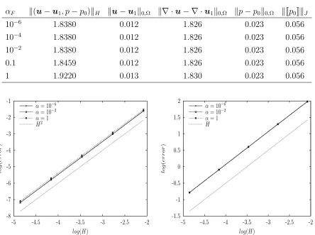
Next, a study of sensitivity of the numerical error with respect toαF is performed in Table
2 for a fixed mesh, where we observe that the errors remain independent of the parameter as long as αF stays of order 1. That agrees with the assumption that τF must be at order
HF, as predicted by the theory. We also perform a convergence study for all the variables
using different values for αF. The results are depicted in Figures 3 and 4 where we can see
that the errors are practically unaffected by the value of αF.
Our next objective is to perform a comparison of the performance of (69) with the lowest order Raviart-Thomas’ mixed finite element methodRT0/QH (cf. [26, 11]). The comparison
[image:27.612.71.540.492.529.2]Table 2. Example I: The sensitivity of the errors with respect to αF.
αF k(u−u1, p−p0)kH ku−u1k0,Ω k∇ ·u− ∇ ·u1k0,Ω kp−p0k0,Ω kJp0KkJ
10−6 1.8380 0.012 1.826 0.023 0.056
10−4 1.8380 0.012 1.826 0.023 0.056
10−2 1.8380 0.012 1.826 0.023 0.056
0.1 1.8459 0.012 1.826 0.023 0.056
1 1.9220 0.013 1.830 0.023 0.056
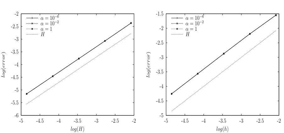
-8 -7 -6 -5 -4 -3 -2 -1
-5 -4.5 -4 -3.5 -3 -2.5 -2
lo
g
(
e
r
r
o
r
)
log(H) α= 10−6
α= 10−2
α= 1 H2
-1.5 -1 -0.5 0 0.5 1 1.5 2
-5 -4.5 -4 -3.5 -3 -2.5 -2
lo
g
(
e
r
r
o
r
)
log(H) α= 10−6
α= 10−2
α= 1 H
Figure 3. Example I: Convergence history for the velocity field (left) and its divergence (right) for different values ofαF.
the mass conservation property foru1+uDe, when the velocity field is updated with uDe, the errors in the divergence are identical. Both methods seem to perform equally good regarding the errors in the pressure field. We want to stress the fact that the solution of (69) involves less degrees of freedom than RT0/QH when the same mesh is used.
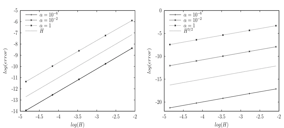
Finally, the unstructured mesh of Figure 7, containing approximately 5000 elements, is adopted. The sensitivity of error in terms of parameter αF presents a different behavior
than before. Nevertheless, since there is a loss of stability whenαF is small, the unexpected
robust error behavior when structured meshes are used is no longer preserved. The results are reported in Table 3 where we observe that the individual norms are not independent of
αF, but the whole k · kH norm of the error seems robust with respect to αF.
-6 -5.5 -5 -4.5 -4 -3.5 -3 -2.5 -2
-5 -4.5 -4 -3.5 -3 -2.5 -2
lo g ( e r r o r )
log(H) α= 10−6
α= 10−2
α= 1 H -5 -4.5 -4 -3.5 -3 -2.5 -2 -1.5
-5 -4.5 -4 -3.5 -3 -2.5 -2
lo g ( e r r o r )
log(h) α= 10−6
α= 10−2
[image:29.612.79.531.83.295.2]α= 1 H
Figure 4. Example I: Convergence history for the pressure (left) and jump
(right) for different values ofαF.
-10 -8 -6 -4 -2 0 2
-6 -5.5 -5 -4.5 -4 -3.5 -3 -2.5 -2
lo g ( e r r o r )
log(H) ku−uRTk0,Ω ku−(u1+uDe)k0,Ω
H2 H -3 -2.5 -2 -1.5 -1 -0.5 0 0.5 1 1.5 2
-6 -5.5 -5 -4.5 -4 -3.5 -3 -2.5 -2
lo g ( e r r o r )
log(H) k∇ ·u− ∇ ·uRTk0,Ω k∇ ·u− ∇ ·(u1+uDe)k0,Ω
H
Figure 5. Example I: Convergence history for the velocity (left) and its
di-vergence (right) for (69) andRT0/QH.
as in the first test, the exact pressure is now p(x, y) =x−x2−1/6 and the velocity field
u= (x2(1−x)2(2y−6y2+ 4y3),−y2(1−y)2(2x−6x2 + 4y3))t.
The source term is then
[image:29.612.83.528.362.556.2]-7 -6.5 -6 -5.5 -5 -4.5 -4 -3.5 -3 -2.5 -2
-6 -5.5 -5 -4.5 -4 -3.5 -3 -2.5 -2
lo
g
(
e
r
r
o
r
)
log(H) kp−pRTk0,Ω kp−p0k0,Ω
H
Figure 6. Example I: Convergence history for the pressure for (69) andRT0/QH.
0 0.1 0.2 0.3 0.4 0.5 0.6 0.7 0.8 0.9 1 0
0.1 0.2 0.3 0.4 0.5 0.6 0.7 0.8 0.9 1
Figure 7. The unstructured mesh.
Table 3. Example I: The sensitivity of the errors with respect to αF using
an unstructured mesh.
αF ku−u1k0,Ω k∇ ·u− ∇ ·u1k0,Ω kp−p0k0,Ω kJp0KkJ k(u−u1, p−p0)kH
10−3 0.6099 1.6741 8.0277 17.6551 1.8843 10−2 0.3017 1.6771 1.8341 2.6921 1.7349 0.1 0.1389 1.6840 0.2585 0.4186 1.6968
1 0.0654 1.7011 0.0373 0.0821 1.7047
10 0.0366 1.8013 0.0228 0.0541 1.8112
and the boundary condition is b = 0. Since the source term f is no longer a constant function in K, we must consider the enhancement of Mu
P
K∈TH(M u
K(−f), σv1)K to the right hand side. From the definition of the operator MuK
we rewrite the right hand side of the equation as
(f,v1)Ω+
X
K∈TH
(σuMe (−f),v1)K = (f,v1)Ω+
X
K∈TH
(−f − ∇pMe (−f),v1)K
= X
K∈TH
(∇pMe (f),v1)K,
werepM
e (f) is solution of the local problem
−∆pMe =−∇ ·f in K, ∂np
M
e =f ·n on ∂K .
(84)
Now, considering the local problems and the conservation mass property, we have∇ ·u1+
∇ ·uDe = 0 at the element level, leading to
∇ ·u1
K =−
1
|K|
X
F∈∂K
αFHF
σ
Z
F
Jp0Kn·nF.
(85)
Hence, we do not expect in general that the error for the divergence of the velocity field to have a good behavior with respect to the parameter αF and we expect a small variation in
the normH since the diverge of the velocity field becomes more important as the parameter
αF is of order one (see Table 5 and Figures 9-10).
The results concerning the errors on velocity and pressure are depicted in Figure 8 using
αF = 0.1. In there we observe a H3/2 convergence for the velocity field in the H(div,Ω)
norm, which is higher than the expected rate of convergence given by the analysis. This is a good thing when we compare to the Raviart-Thomas method, in which the discrete velocity field is exactly divergence-free. Of course, when updated with the enrichment function uD
e ,
then the velocity field becomes exactly divergence-free (see Table 4 for the mass-conservation results). The sensitivity of the error with respect toαF is performed in Table 5, and as before,
we study the convergence of the method for different choices ofαF and we report the results
[image:31.612.71.540.619.655.2]in Figures 9 and 10 where we observe that the errors in divergence are affected by the value of αF, while the rest seem fairly independent ofαF.
Table 4. Example II: Relative local mass conservation error.
H 6.25×10⁻² 3.12×10⁻² 1.56×10⁻² 7.8×10⁻³ 3.9×10⁻³
Me 1.04×10⁻¹⁵ 1.03×10⁻¹⁵ 9.11×10⁻¹⁵ 1.41×10⁻¹⁴ 6.30×10⁻¹⁵
Now we perform a comparison of (69) with the lowest order Raviart-Thomas’ mixed method RT0/QH where we get better precision for the velocity field, as before, and the
-16 -14 -12 -10 -8 -6 -4
-6 -5.5 -5 -4.5 -4 -3.5 -3 -2.5 -2
lo
g
(
e
r
r
o
r
)
log(H) ku−u1k0,Ω
k∇ ·u− ∇ ·u1k0,Ω
H2
H3/2
-9 -8.5 -8 -7.5 -7 -6.5 -6 -5.5 -5 -4.5 -4 -3.5
-6 -5.5 -5 -4.5 -4 -3.5 -3 -2.5 -2
lo
g
(
e
r
r
o
r
)
log(H) kp−p0k0,Ω
kJp0KkJ
[image:32.612.86.526.99.294.2]H
Figure 8. Example II: Convergence history for the velocity field and its
di-vergence(left) and the pressure and jump (right).
Table 5. Example II: The sensitivity of errors with respect to αF.
αF k(u−u1, p−p0)kH ku−u1k0,Ω k∇ ·u− ∇ ·u1k0,Ω kp−p0k0,Ω kJp0KkJ
10−6 0.0090 5.7×10⁻⁵ 4.6×10⁻⁹ 0.003 0.006 10−4 0.0090 5.7×10⁻⁵ 4.6×10⁻⁷ 0.003 0.006 10−2 0.0090 5.7×10⁻⁵ 4.6×10⁻⁵ 0.003 0.006 0.1 0.0094 6×10⁻⁵ 4.6×10⁻⁴ 0.003 0.006 1 0.0013 1.9×10⁻⁴ 4.6×10⁻³ 0.003 0.006
5.3. The five-spot problem. Due to its practical importance in oil recovery, the quarter five spot problem has served as a paradigm to validate stability and accuracy of numerical methods for the Darcy model. This problem is now addressed considering zero source term
f and σ = 1 in a unit square domain, and instead of modeling injection and production
of well by a non-zero source term g, we consider a non-homogeneous boundary condition for the velocity such that its normal component is equal to 4H1F at points (0,0) and (1,1). This delta of Dirac is linearly approached on the edges sharing such points. The solution obtained is depicted in Figures 12-15 where we observe the total absence of oscillations in the solution. The constantαF is again fixed equal to 0.1. In Table 6 we study the local mass
[image:32.612.89.524.396.504.2]-14 -13 -12 -11 -10 -9 -8 -7 -6 -5
-5 -4.5 -4 -3.5 -3 -2.5 -2
lo g ( e r r o r )
log(H) α= 10−6
α= 10−2
α= 1 H -20 -15 -10 -5 0
-5 -4.5 -4 -3.5 -3 -2.5 -2
lo g ( e r r o r )
log(H) α= 10−6
α= 10−2
[image:33.612.76.531.88.294.2]α= 1 H3/2
Figure 9. Example II: Convergence history for the velocity field (left) and
its divergence (right) for different values of αF.
-8 -7.5 -7 -6.5 -6 -5.5 -5 -4.5 -4
-5 -4.5 -4 -3.5 -3 -2.5 -2
lo g ( e r r o r )
log(H) α= 10−6
α= 10−2
α= 1 H -7 -6.5 -6 -5.5 -5 -4.5 -4 -3.5
-5 -4.5 -4 -3.5 -3 -2.5 -2
lo g ( e r r o r )
log(H) α= 10−6
α= 10−2
[image:33.612.82.528.357.548.2]α= 1 H
Figure 10. Example II: Convergence history for the pressure (left) and jump (right) for different values ofαF.
Table 6. Five spot problem: Relative local mass conservation error
h 6.25×10⁻² 3.12×10⁻² 1.56×10⁻² 7.8×10⁻³ 3.9×10⁻³
Me 4.11×10⁻¹² 2.3×10⁻¹² 7.29×10⁻¹² 1.34×10⁻¹¹ 1.32×10⁻⁹
6. conclusion
[image:33.612.80.543.625.661.2]-16 -14 -12 -10 -8 -6 -4
-6 -5.5 -5 -4.5 -4 -3.5 -3 -2.5 -2
lo g ( e r r o r )
log(H) ku−uRTk0,Ω ku−(u1+uDe)k0,Ω
H2 H -9 -8.5 -8 -7.5 -7 -6.5 -6 -5.5 -5 -4.5 -4
-6 -5.5 -5 -4.5 -4 -3.5 -3 -2.5 -2
lo g ( e r r o r )
log(H) kp−pRTk0,Ω kp−p0k0,Ω
[image:34.612.77.531.101.294.2]H
Figure 11. Example II: Convergence history for the velocity (left) and for
the pressure (right) for (69) and RT0/Q0H.
0 0.1 0.2 0.3 0.4 0.5 0.6 0.7 0.8 0.9 1 0 0.1 0.2 0.3 0.4 0.5 0.6 0.7 0.8 0.9 1 −0.6 −0.4 −0.2 0 0.2 0.4 0.6 0.8 −0.4 −0.2 0 0.2 0.4 0.6
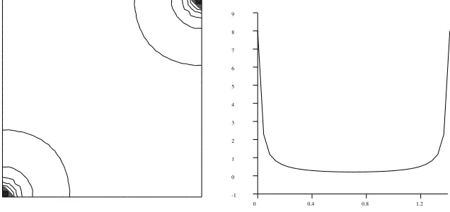
Figure 12. Five spot problem: Profile of pressure.
[image:34.612.150.437.362.520.2]0 0.1 0.2 0.3 0.4 0.5 0.6 0.7 0.8 0.9 1 0
0.1 0.2 0.3 0.4 0.5 0.6 0.7 0.8 0.9 1
−0.4 −0.2 0 0.2 0.4 0.6
Figure 13. Five spot problem: Isovalues of the pressure.
0 0.1
0.2 0.3
0.4 0.5
0.6 0.7
0.8 0.9
1
0 0.1 0.2 0.3 0.4 0.5 0.6 0.7 0.8 0.9 1 0 2 4 6 8 10 12
1 2 3 4 5 6 7 8 9 10 11
Figure 14. Five spot problem: The 2-norm of the velocity.
the boundary condition for the local problems ought to include further control on the gra-dient of the pressure. Finally, enriched methods seem to show an intrinsic relationship with some discontinuous finite element methods. This subject should be enrolled in forthcoming works.
Acknowledgments
0 0.4 0.8 1.2 -1
[image:36.612.147.465.108.258.2]0 1 2 3 4 5 6 7 8 9
Figure 15. Five spot problem: Isovalues for |u1| and a cross-section along
the liney=x.
the NSF/USA Grant No. 0610039. The authors want to thank Leopoldo Franca and Rodolfo Rodr´ıguez for many helpful discussions and comments.
References
[1] R. Araya, G. R. Barrenechea, L. P. Franca, and F. Valentin, Stabilization arising from PGEM: A review and further developments. Applied Numerical Mathematics, to appear, 2008.
[2] R. Araya, G. R. Barrenechea, and F. Valentin, Stabilized finite element methods based on multiscale enrichment for the Stokes problem, SIAM J. Numer. Anal., 44 (2006), pp. 322–348.
[3] T. Arbogast,Analysis of a two-scale locally conservative subgrid upscaling for elliptic problems, SIAM J. Numer. Anal., 42 (2004), pp. 576–598.
[4] C. Baiocchi, F. Brezzi, and L. P. Franca,Virtual bubbles and Galerkin-Least-Squares type methods (Ga.L.S.), Comput. Methods Appl. Mech. Engrg., 105 (1993), pp. 125–141.
[5] G. R. Barrenechea, L. P. Franca, and F. Valentin,A Petrov-Galerkin enriched method: a mass conservative finite element method for the Darcy equation, Computer Methods in Applied Mechanics and Engineering, 196 (2007), pp. 2449–2464.
[6] ,A symmetric nodal conservative finite element method for the Darcy equation. Preprint 2008-07, Department of Mathematics, University of Strathclyde, 2008.
[7] G. R. Barrenechea and F. Valentin,An unusual stabilized finite element method for a generalized Stokes problem, Numer. Math., 92 (2002), pp. 653–677.
[8] , Relationship between multiscale enrichment and stabilized finite element methods for the gener-alized Stokes problem, CRAS, 341 (2005), pp. 635–640.
[9] P. B. Bochev and M. D. Gunzburger,A locally conservative least-squares method for Darcy flows, Comm. Numer. Methods Engrg., 24 (2008), pp. 97–110.
[11] F. Brezzi and M. Fortin, Mixed and Hybrid Finite Element Methods, vol. 15 of Springer Series in Computational Mathematics, Springer-Verlag, Berlin, New-York, 1991.
[12] F. Brezzi, L. Franca, T. J. Hughes, and A. Russo, Stabilization techniques and subgrid scale capturing, in Proceedings of the Conference “The State of the Art in Numerical Analysis”, York, 1–4 April, 1996, I. Duff, ed., IMA Conference, Oxford University Press, 1997.
[13] F. Brezzi, L. P. Franca, and A. Russo, Further considerations on Residual-Free Bubbles for advective-diffusive equations, Comput. Methods Appl. Mech. Engrg., 166 (1998), pp. 25–33.
[14] F. Brezzi and A. Russo, Choosing bubbles for advection-diffusion problems, Math. Models Methods Appl. Sci., 4 (1994), pp. 571–587.
[15] E. Burman and P. Hansbo,A unified stabilized method for Stokes’ and Darcy’s equations, J. Comput. Appl. Math., 198 (2007), pp. 35–51.
[16] Z. Chen and T. Hou,A Mixed Multiscale Finite Element Method for Elliptic Problems with Oscillating Coefficients, Mathematics of Computation, 72 (2003), pp. 541–576.
[17] P. Cl´ement, Approximation by finite element functions using local regularization, RAIRO Anal. Num´er., (1975), pp. 77–84.
[18] W. E and B. Engquist,The heterogeneous multiscale methods, Commun. Math. Sci., 1 (2003), pp. 87– 132.
[19] A. Ern and J.-L. Guermond, Theory and Practice of Finite Elements, Springer-Verlag, 2004. [20] L. P. Franca, A. L. Madureira, L. Tobiska, and F. Valentin, Convergence analysis of a
multiscale finite element method for singularly perturbed problems, SIAM Multiscale Model. and Simul., 4 (2005), pp. 839–866.
[21] L. P. Franca, A. L. Madureira, and F. Valentin,Towards multiscale functions: enriching finite element spaces with local but not bubble–like functions, Comput. Methods Appl. Mech. Engrg., 194 (2005), pp. 3006–3021.
[22] L. P. Franca, A. Nesliturk, and M. Stynes,On the stability of residual-free bubbles for convection-diffusion problems and their approximation by a two-level finite element method, Comput. Methods Appl. Mech. Engrg., 166 (1998), pp. 35–49.
[23] V. Girault and P. A. Raviart, Finite Element Methods for Navier-Stokes Equations: Theory and Algorithms, vol. 5 of Springer Series in Computational Mathematics, Springer-Verlag, Berlin, New-York, 1986.
[24] T. J. R. Hughes, G. R. Feijoo, L. Mazzei, and J. Quincy,The variational multiscale method - a paradigm for computational mechanics, Computer Methods in Applied Mechanics and Engineering, 166 (1998), pp. 3–24.
[25] L. E. Payne and H. F. Weinberger, An optimal Poincar´e inequality for convex domains, Arch. Rational Mech. Anal., 5 (1960), pp. 286–292.