Framework for optimizing intelligence collection requirements

Rochester Institute of Technology

RIT Scholar Works

Theses

Thesis/Dissertation Collections

11-1-2010

Framework for optimizing intelligence collection

requirements

Khiem Tong

Follow this and additional works at:

http://scholarworks.rit.edu/theses

This Thesis is brought to you for free and open access by the Thesis/Dissertation Collections at RIT Scholar Works. It has been accepted for inclusion in Theses by an authorized administrator of RIT Scholar Works. For more information, please [email protected].

Recommended Citation

Framework for Optimizing Intelligence Collection Requirements

by

Khiem Duy Tong

A Thesis Submitted in Partial Fulfillment of the Requirements for the Degree of Master of Science in Computer Engineering

Supervised by

Rochester Institute of Technology Dr. Shancieh Jay Yang Department of Computer Engineering

Kate Gleason College of Engineering Rochester Institute of Technology

Rochester, New York November 2010

Approved By:

Dr. Shancieh Jay Yang

Rochester Institute of Technology Primary Adviser

Dr. Moises Sudit University at Buffalo

Dr. Andres Kwasinski

Thesis Release Permission Form

Rochester Institute of Technology Kate Gleason College of Engineering

Title: Framework for Optimizing Intelligence Collection Requirements

I, Khiem Duy Tong, hereby grant permission to the Wallace Memorial Library to reproduce my

thesis in whole or in part.

Khiem Duy Tong

Dedication

Acknowledgments

I would like to express my gratitude to Dr. Shanchieh Jay Yang for his mentorship, without whose

help and inspiration I would never have finished this work.

I would like to thank Dr. Moises Sudit, Dr. Andres Kwasinski, and Jared Holsopple for their

valuable advice.

Lastly I would like to acknowledge CUBRC and AFRL for providing the financial funding needed

Glossary

A

AOI Area of Interest, p. 7.

C

COA Course of Action, sequence of actions that can be performed, p. 1.

CRAs Collection Requirement Actions, actions that are performed to collect intelligence, p. 2.

D

decision support model, tools, or processes which can aid effective decision making, p. 1.

DM Decision Maker, individual with responsibility of making decisions in an operation or

mission, p. 1.

DSS Decision Support System, systems which model, analyze, or visualize information to

aid effective decision making, p. 1.

G

GUI Graphical User Interface, p. 12.

J

JIPOE Joint Intelligence Preparation of the Operational Environment, analytical process used

P

PF Plausible Future, any event or set of events that could occur in future as anticipated by

Abstract

In the military, typical mission execution goes through cycles of intelligence collection and action

planning phases. For complex operations where many parameters affect the outcomes of the

mis-sion, several steps may be taken for intelligence collection before the optimal Course of Action is

actually carried out. Human analytics suggests the steps of: (1) anticipating plausible futures, (2)

determining information requirements, and (3) optimize the choice of feasible and cost-effective

intelligence requirements. This work formalizes this process by developing a decision support tool

to determine information requirements needed to differentiate critical plausible futures, and

formu-lating a mixed integer programming problem to trade-off the feasibility and benefits of intelligence

collection requirements.

Course of Action planning has been widely studied in the military domain, but mostly in an

abstract fashion. Intelligence collection, while intuitively aiming at reducing uncertainties, should

ultimately produce optimal outcomes for mission success. Building on previous efforts, this work

studies the effect of plausible futures estimated based on current adversary activities. A set of

differentiating event attributes are derived for each set of high impact futures, forming a candidate

collection requirement action. The candidate collection requirement actions are then used as inputs

to a MIP formulation, which optimizes the plausible future mission state subject to timing and

cost constraints. The plausible future mission state is estimated by assuming that the CRAs can

potentially avert the damages adversary future activities might cause. A case study was performed

Contents

Dedication . . . . iii

Acknowledgments . . . . iv

Glossary . . . . v

Abstract . . . . vii

1 Introduction. . . . 1

2 Understanding the Problem . . . . 3

2.1 Generalized Information Flow Model . . . 3

2.2 Analytical Processes . . . 6

2.3 Automated Tools . . . 8

2.3.1 INFERD . . . 8

2.3.2 FuSIA . . . 9

2.4 Subjective Assessments and Hierarchal Modeling of Missions . . . 10

2.5 Problem in Perspective . . . 12

3 Intelligence Collection Framework. . . . 14

3.1 Determining CRAs from Plausible Futures . . . 17

3.1.1 Identification of critical plausible futures . . . 21

3.1.2 Analysis of plausible futures using attributes . . . 24

3.1.3 Ranking plausible futures . . . 24

3.2 Evaluating Mission Impact Using CRA Matrices . . . 26

3.3 Aggregation Functions . . . 28

3.3.1 Ordered Weighted Average . . . 29

3.4 Optimization Formulation . . . 29

3.4.1 Logical Constraints . . . 31

4 Case Study . . . . 36

4.1 Scenario: Hostage Rescue . . . 36

4.2 Results . . . 42

4.3 Limitations . . . 42

5 Conclusion and Future Work. . . . 45

5.1 Future Work . . . 45

5.1.1 Fully integrated decision support system . . . 45

5.1.2 Exploring feedback in collection requirements . . . 45

5.1.3 Generalizing framework to other domains . . . 46

List of Figures

2.1 Generalized informatin flow model [28] . . . 4

2.2 Decision state matrix [27] . . . 6

2.3 Effects Based Planning model . . . 10

2.4 Example cross impact matrix [19] . . . 11

3.1 Intelligence collection framework flow . . . 14

3.2 Example of gathering plausible futures from a database . . . 19

3.3 Plausible futures conversion tool . . . 20

3.4 Configuring and display of important attributes . . . 22

3.5 Determining which attributes affect plausible futures most . . . 23

3.6 Analysis of sets of plausible futures . . . 25

3.7 Ranking of plausible futures based on attributes . . . 26

3.8 Example CRA matrix . . . 26

3.9 Representing current and future asset states . . . 27

3.10 Mission hierarchy tree. . . 28

3.11 Gurobi implementation of logical max constraint . . . 33

4.1 Attribute-based analysis of plausible futures . . . 37

4.2 Future impact matrix . . . 38

List of Tables

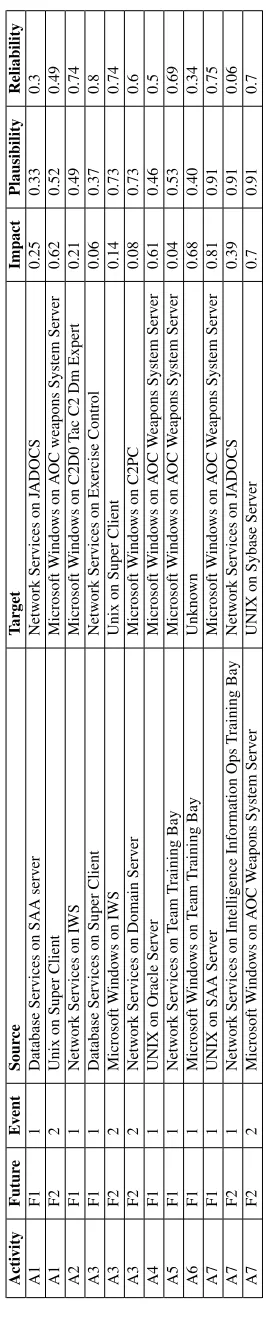
3.1 Example plausible futures . . . 18

Chapter 1

Introduction

In the military domain, missions are defined to accomplish goals which can require complex

de-cisions. As a result decision making has been studied extensively in the military to establish

doc-trine [3, 7, 16]. The fundamental notion in these works is the iterative cycle of Course of Action

(COA) development, determination of which COA(s) to adopt, and implementation of COA(s) [23].

Intelligence collection plays a crucial role in all three fundamental phases; better intelligence

collection improves decision maker’s (DM’s) and analyst’s ability to develop and adopt effective

COAs. In turn, intelligence collection requires its own set of steps: (1) anticipating plausible futures

(PF), (2) determining information requirements, (3) optimizing collection based on feasibility and

cost-effectiveness.

These steps are not trivial and along with the need for intelligence collection at the

strate-gic, tactical, and operational level present a challenging problem for analysts [13]. The number

of parameters and expert knowledge required to effectively carry out intelligence collection

sug-gests the need for decision support. Decision support systems (DSS) are computerized tools which

provide decision support by supplying information that can reinforce and improve a DM’s

effec-tiveness [14, 17, 20]. DSS have been implemented in many different domains such as in supply

chains [2, 5], medicine [6], information fusion [15], and some existing military applications [14].

However, to properly offer decision support an understanding of the intelligence collection

process is required. Intelligence collection has been studied extensively as analytical processes.

Hutchinset al.[10] work on the Tactical Decision Making Under Stress (TADMUS) program cover

the principles that are needed for decision support with regards to navy ships operating in littoral

(coastline) regions of world. Where challenges such as closer proximity to enemies and swiftly

performed by humans in these military operations and subsequently discussed how decision support

and (human-system) interaction design could be used to reduce the cognitive requirement on a

deci-sion maker. It was found that DSS could not adequately replicate expertise gained from experience.

Since all contingencies in a situation cannot be anticipated, a human expert’s intuition is needed.

However, DSS can reduce search time for relevant information through graphical presentations, and

reduce amount of cognitive computation required for certain tasks. This project suggests that the

use of DSS can prove beneficial in a military context.

This research builds off previous works to develop a formal decision support framework for

intelligence collection. The framework is composed a decision support tool that determines

infor-mation requirements needed to differentiate between critical plausible futures and a mixed integer

programming (MIP) optimization formulation that can trade-off between the feasibility and benefits

of different intelligence requirements. In essence the the effort allows for analysts to differentiate

between plausible futures via attributes to craft candidate collection requirement actions (CRAs). A

set of optimal collection requirement actions are produced via the MIP formulation that can guide

Chapter 2

Understanding the Problem

Providing decision support for intelligence collection requires a thorough understanding of the

intel-ligence collection process. Several works were critical in building the foundation needed to properly

interpret the problem.

2.1

Generalized Information Flow Model

Yovitset al. [27, 28] work on the Generalized Information Flow Model acted as a starting point.

As shown in Figure 2.1, Yovits tries to capture the ability of a DM to learn and adapt over time.

Yovits’ model relies on three hypotheses: (1) information is data of value in decision-making, (2)

information gives rise to observable effects, and (3) information feedback exists so that the DM will

adjust his model for later decisions.

A fundamental idea in this model is that the two sources of information come from the

envi-ronment and from feedback based on observations of results from previous decisions (e.g. DM’s

experience). In this model, information is captured from the environment through a process called

Information Acquisition and Dissemination (IAD). This is simply the process by which sensors

capture data and this data is propagated to the analysts and DMs. This information is processed

and provided as input to the decision maker. The decision maker uses the information available

to choose a COA. The COA is executed and the results are observed. These results are compared

against anticipated results and transformed into data that can be used in a feedback loop at the IAD

stage. In this way the DM learns about how decisions and outcomes are related and can adjust

accordingly.

Environment

Information Acquisition and Dissemination (IAD)

Decision-Making Execution (E)

Transformation (T)

Environment

Observables Courses of

Action Information

Data

Figure 2.1: Generalized informatin flow model [28]

from the information available to them (from the environment and experience). These two elements

are representative of the natural elements in human decision making: considering the current

en-vironment and anticipating future events. The generalized decision making process according to

Yovits is given below:

1. DM makes a decision (chooses a COA) on the basis of all information available.

2. DM predicts some probable outcomes.

3. A comparison is made between observed results and anticipated results (feedback).

4. Updates the model of the situation from results observed.

5. Return to step 1.

Yovits asserts that DMs will always try to fulfill two main objectives: choose the best COA

and learn as much as possible about the current situation. Yovits states that while classical decision

making maintains that DMs will always choose to prioritize the former, this is an

or wanting to learn more about the current situation. Thus, intelligence plays a critical role in the

mission planning process and selection of COAs.

Yovits also emphasizes the vital role of uncertainty in decision making and categorizes it into

three categories: (1) state of nature uncertainty, (2) executional uncertainty, and (3) goal

uncer-tainty. State of nature uncertainty is the result of uncontrollable external conditions that could

influence outcomes. Examples of state of nature include: weather, governmental regulation,

econ-omy, etc. Executional uncertainty refers to the unknowns arising from DMs identifying available

COAs (options) and outcomes of the COAs. Yovits asserts that the relationship between COAs and

outcomes are probabilistic and not deterministic (even with known state of nature). Finally goal

uncertainty arises from DMs having to consider outcomes and the influence they have on the end

goal. Intelligence collection can be seen as a way to resolve these uncertainties to reach end goals.

As part of this work, a matrix representation was used capture a DM’s decision state [28].

Figure 2.2 shows an example decision state matrix where am are COAs, on are outcomes, ω_ijk is

a probabilistic measure, andvk(on) are the effective values of the outcomes. Effective values are

defined as the rating of how much an outcome moves the situation towards a desired end goal.

The values of ω are subjective probabilistic measures that relate COAs to outcomes. Using this

representation allows a DM to accomplish their two main tasks of choosing the best COA and

learning about the situation. To choose the best COA a DM tries to maximize the sum of the

effective values of the outcomes. The DM can also use the matrix to learn more about the situation

by reviewing thewij values. This allows the DM to see which COA they are most uncertain about

(i.e.,those with lowwij values).

Llinas [12] builds off Yovits’ work to develop the conceptual idea of a mathematical

program-ming based optimization problem to model the decision making process. Llinas states that when

selecting a COA a DM is basically defining a task to be carried out. The next logical step requires

determining what kind of resources can be used to feasibly perform the tasks. Finally a DM must

select the best or optimal resource to perform the tasks. This leads to the idea of an optimization

problem. The outputs of this optimization problem are the resources that should be employed to

carry out the COA.

In summary, Yovits developed a generalized model for the decision making process and ways

Relative Values vk(o1 vk(o2) . . . vk(oj) . . . vk(on)

Outcomes o1 o2 . . . oj . . . on

Courses of action

a1 w11k wk12 . . . wk1j . . . wk1n a2 w21k wk22 . . . wk2j . . . wk2n

. . . .

. . . .

. . . .

ai w_ik₁ wk_i2 . . . wk_ij . . . wk_in

. . . .

. . . .

. . . .

am wk_m1 w_mk₂ . . . w_mjk . . . w_mnk

Figure 2.2: Decision state matrix [27]

is possible to use a mathematical programming based optimization problem to help achieve mission

success.

2.2

Analytical Processes

There is existing doctrine which define analytical approaches to the creation and selection of COAs

in the military domain. Previous efforts have also created automated tools that generate plausible

futures.

Joint Intelligence Preparation of the Operational Environment [16] (JIPOE) is a systematic

(structured) analytical process employed by the joint intelligence organizations. The operational

environment refers to the set of conditions, circumstances, and factors that can affect a decision

maker. The JIPOE process aims to provide a holistic view of the operational environment by

char-acterizing pertinent information with regards to air, land, maritime, space, and cyberspace domains.

The breadth and diversity of the domains require a large amount of subject matter expertise [16].

The analytical process will usually involve experts from several different agencies and allies

coop-erating together. There are four steps in the JIPOE process:

1. Define the operational environment,

2. Describe the impact of the operational environment,

4. Determine the adversary COAs

JIPOE is cyclical in nature and similar to Yovits’ model reflects how analysts must constantly

learn and adapt.

The first step in the JPIOE process is to define the operational environment [16]. The analysts

identify the operational area and the characteristics of the operational environment that are relevant

to the mission. They must keep the intent of the commander in mind to accomplish this. The analysts

must define the bounds of the areas of interest (AOI), both physical and non-physical. A trade-off

must be considered by analysts to determine what level of detail is needed and the amount of time

that is available to accomplish it. This step also involves the analyst figuring out the intelligence

gaps, priorities and shortfalls. As evidenced there are a large number of factors even within this

initial step. In step two of JPIOE the impact of the operational environment is described. This

involves considering all of the potential factors that could impact operations. For example how will

climate, weather, sociocultural, and other factors impact operations. Also in this step the analyst

must understand the relationships in the operational environment from a systems perspective, how

the elements are connected and what interactions they have.

In the third step of the JPIOE process the adversary must be evaluated [16]. This is a procedure

where the analysts must identify capabilities, limitations, doctrine, patterns of operation, tactics

and techniques of the adversary. This space is constrained by the factors identified in step two of

the process which reduces the possibilities based on the operational environment. Still it can be

seen that the considerations that an analyst must make are significant. An analyst must consider

adversary capabilities and define COAs that they can use to interfere with Blue’s (the friendly)

mission. 2 In the fourth step the adversary COAs are determined [16]. The holistic view that has

been built up through the previous steps is put to use and an understanding of the the adversary’s

intent and strategy is developed. The analysts identify what the adversary’s goal and objectives

are. The analyst must then consider and create the full set of adversary COAs. Once the set of

COAs have been created the analyst goes on to prioritize (rank) the COAs in order of probability

of adoption. Effectively predicting what the likely set of actions the adversary will take. Given the

amount of time that was determined in the previous step the analysts flesh out as much detail for

each COA as possible. Finally the analysts identify initial collection requirements. This is used to

adopted, effectively determining friendly (Blue) COAs.

JIPOE provides a doctrinal approach to mission planning that revolves around establishment

and selection of COAs. Intelligence collection provides the essential ingredient needed for success

in both phases.

Intelligence Preparation of the Battlefield (IPB) is another analytical process for threat

assess-ment, and understanding of the environment in a geographic area [3]. The main purpose of IPB is

similar to that of JPIOE as both are designed to support analyst and commander’s decision

mak-ing [3]. In essence IPB is the description of the effects of the battlefield and determination of the

threat’s COA to determine a friendlies best COA.

The main functions that are performed during IPB are essentially the same as those in JPIOE

except at a finer detail. They differ specifically in their focus, JPIOE is designed to help the

com-mander at the overall mission level whereas IPB and its finer degree of detail supports component

command operations. JPIOE and IPB can be used together however these two processes should not

overlap [16]. IPB can be extremely detailed, for example an individual soldier can informally

per-form IPB when he considers the possible actions of an enemy soldier he is about to engage. JPIOE

will usually be performed at a higher level.

2.3

Automated Tools

2.3.1 INFERD

INformation Fusion Engine for Real-time Decision-making (INFERD) is a stream based processing

system to update track estimates in real time as sensor messages are fed in as input [22]. The tracks

used in INFERD are semantic or contextual and not kinematic and can be viewed a grouping of

correlated events [22]. The system’s architecture was designed to function in different domains.

Two sets of inputs are provided as inputs for INFERD: a priori models, and runtime sensor data

(measurement). These inputs are used in an information flow consisting of:

1. Data Alignment

2. Connotation Elicitation

4. Track Update and Reporting

First sensor data from diverse sources are written to a database which is then read by INFERD.

The data then goes through Data Alignment, a preprocessing step to homogenize the data [22].

This is done through a wrapper which converts each type of sensor message into a common format

used by INFERD. Next in Connotation Elicitation, theSensor Messageis used to create anElicited

Message which is simply a Sensor Message with an additional Model Connotation Layer [22].

This is additional information generated using thea priorimodels provided to add more meaning

to the sensor data. This could be viewed as classifying messages based on their attributes into

categories. In the following step, Data Association, an estimate is made to determine which track

the measurement is a part of. In addition to this, how does the new measurement associate with the

existing track. The cardinality of the set of feasible tracks and elements that are produced by the

data association stage is used to decide which of three kinds of processing the Track Update module

takes [22]:

1. If an Elicited Message is not associated to any track, a new track is created.

2. If it’s associated with a single track, message is added to that track.

3. If associated to multiple tracks, a hyper track will be created and the possible predecessor

tracks are linked.

In essence, INFERD is an automated system which produces estimates of adversary activities

by correlating observations and usinga prioriknowledge.

2.3.2 FuSIA

Future Situation and Impact Awareness (FuSIA) [8] is a generalized threat assessment framework

applied specifically to cyber security that is able to estimate plausible presents and futures in a

de-fined environment. FuSIA is not a predictor of future events; plausible futures are simply generated

and assigned a rating.

FuSIA takes input in the form of attack tracks. The futures are generated using an ontology that

represents the relationships between objects and activities in the attack tracks. Three algorithms

aspects separately and then combines them to generate plausible futures. A plausibility score is

assigned for each generated future. The plausibility score that FuSIA generates is not a probability

[8]. Plausibility scores do not have to sum to one across all the possible generated futures and is

only a rating based on the current available evidence.

JIPOE, FuSIA, and INFERD provide stepping stones for formalizing the intelligence collection

process as a framework. They offer components that are needed to develop a DSS for intelligence

collection.

2.4

Subjective Assessments and Hierarchal Modeling of Missions

A2

A3 A1

A7 A6 A5 A4 SE2

SE3 SE1

SE5 SE4 DC1

DC2 MES

Figure 2.3: Effects Based Planning model relating Military End State (MES), Decisive Conditions (DC), Supporting Effects (SE), and Actions (A) [18]

Schubert et al. [9, 18, 19] formulated a subjective assessment method for mission planning,

specifically in Effects Based Planning [21]. In EBP, a hierarchal plan is constructed relating Military

Figure 2.4: Example cross impact matrix [19]

shown in Figure 2.3. The Military End State is the desired end goal of the plan. A Decisive

Condition is a condition required for a transition between its phases. Supporting Effects are effects

that are associated with one or many DCs. Finally, Actions are activities needed to fulfill one or

many SEs. A CIM, as shown in Figure 2.4, is created in the initial planning process by subject

matter experts (SMEs) as required by the type of operation. These SMEs assess how each element

of the EBP process can affect each other, all the way up to the Military End State. In the CIM

approach only the direct first-order influences for each object (DC, SE, A) are considered. Objects

that are on the same level can influence each other bidirectionally while those on different levels are

limited to unidirectional influence. The idea of influences also leads to the idea of multiplicative

effects (sum of influences is greater than individual influence) which is not modeled in the CIM

approach. The values in the CIM denote the influence ranging from -9 (negative influence) to 9

(positive influence) and are assigned by the aforementioned SMEs. Analysis of the CIM can lead to

discovery of previously unseen synergies, alternatives, and conflicts [19].

A Collaborative Synchronization Management Tool (CSMT) was developed [9] which

by SMEs and display various views of the data via a graphical user interface. This simplifies the

analysis process by presenting the data within a graphical user interface (GUI)allowing easier

ma-nipulation and interaction. The views are displays of the results of processing on the data provided

by the user.

2.5

Problem in Perspective

In the military domain missions are carefully planned out and executed following a process which

revolves around the creation of both adversary and friendly COAs. Existing analytical processes

such as JIPOE [16] and IPB [3] define precise procedures for analysts and commanders to carry

out these tasks. Intelligence collection is vital to both of these activities and requires a prescribed

process itself. Due to the complexity of intelligence collection, decision support is desirable [10,

14, 15]. However, to provide proper decision support an understanding of the intelligence collection

process and its components is required.

Yovits’ [27, 28] and Llinas’ [12] showed that intelligence collection revolves around reducing

uncertainty. This is done by organizing collection requirements and performing collection activities.

Yovits provided a generalized model by which this could be done. The fundamental idea ind Yovits’

model is that information comes from two main sources, the environment and analyst experience.

This information provides DMs with the options available to them. Improved quality of information

provides a DM with more options and an improved ability to make better decisions. Llinas’ builds

off Yovits’ work and suggests that mathematical optimization could be used to find optimal sets of

actions to be performed to gather intelligence.

Thus, to provide decision support information sources that conform to the categories of

envi-ronmental information (collected by sensors) and experiential (analytical) information are needed.

JIPOE and IPB are analytical processes employed by the military and can provide the analytical

components needed. INFERD [22] and FuSIA [8] are automated tools developed previously that

process sensor data and can provide the type of environmental data required.

A model was needed in order to evaluate the influences of the data from the information sources.

Schubert’s work [9, 18, 19] formalized a subjective assessment method for mission planning. This

level factors could influence a mission. The use of a hierarchy required appropriate algebraic

repre-sentation and aggregation functions were found to be appropriate for combining influences as they

were propagated in the hierarchy [1].

This effort ties together these ideas with novel contributions to develop an intelligence collection

Chapter 3

Intelligence Collection Framework

The overall structure of the intelligence collection requirements framework is shown in Figure 3.1.

The framework is composed of two main components: a plausible futures tool, and an optimization

formulation. The plausible futures tool is an application that allows for attribute based analysis of

plausible futures. Candidate CRAs can be derived from such analysis. These CRAs are then used in

an MIP optimization formulation to select the best CRA by trading off feasibility and effectiveness.

The end result is an optimized set of CRAs that can be used to aid DMs in their decision making.

However there are several challenges that first need to be overcome:

• How can collection requirements be determined from plausible futures?

• How can the resulting collection requirements be represented so that they can be optimized?

• Implementing the optimization problem.

Before these challenges can be tackled an understanding of the intuition behind the framework

is required. This starts with understanding what exactly are plausible futures and CRAs.

Candidate CRAs

Optimized CRAs PF Analysis Tool

Plausible Futures

Optimization

Figure 3.1: Intelligence collection framework flow

Plausible futures are likely adversary actions that can come from analytical processes such as

futures and COAs is that plausible futures is a loosely defined term that can refer to individual

actions or a generic set of actions whereas COAs strictly refer to a sequence of actions. Plausible

futures can be represented as a set of characteristic attributes that are domain dependent. For this

work the attributes used include:

1. ID

2. Name

3. Source

4. Target

5. Impact

A mission can be defined as a set of actions with associated assets that are responsible for their

completion [12]. These assets each have a current state which measures the ability of these assets

to complete a task. Consider i assets responsible for carrying out actions in a mission with the

relationship between assets and actions being defined by analysts. Acurrent impact matrix(Sc) can

be defined which associates theiassets with a current state as shown.

Sc=               state

a1 0.0

a2 0.0

a3 0.0

a4 0.0

a5 0.0

             

Analysts can consider plausible futures each of which can impact the assets. The impact value

is a subjective measure ranging from 0.0 (no effect) to 1.0 (maximum effect) conveying how a

plausible future influences the health of assets. Consideriassets andj plausible futures, afuture

futures can be associated with different adversaries. Thus, the j columns can be associated any

combination of adversaries.

Sf =

             

p1 p2 p3 p4 p5

a1 0.1 0.0 0.0 0.3 0.15

a2 0.24 0.2 0.0 0.6 0.0

a3 0.33 0.0 0.0 0.73 0.0

a4 0.05 0.8 0.55 0.0 0.23

a5 0.9 .67 .34 0.8 0.0

             

A Collection Requirement Action (CRA) is an action that can be taken mitigate impact from

plausible futures. These actions are defined by analysts from domain knowledge. A CRA can be

defined as a binaryCRA matrix(CRAn(i, j)) which associates plausible futures to assets that they

affect. This allows for differentiation between candidate actions that can be taken as each action

will correspond to plausible future-asset pairs. There can be overlaps in plausible future-asset pairs

between CRAs. The monitoring state of plausible future-asset pairs across all selected CRAs is

aggregated to form a single matrix (α(i, j)), whereα(i, j) =max(CRAn(i, j)),∀i, j, n.

CRAn(i, j) =

             

p1 p2 p3 p4 p5

a1 0 0 0 0 0

a2 0 1 1 0 0

a3 0 0 0 0 0

a4 0 0 0 0 0

a5 0 0 0 0 0

             

During mission planning there may be a large number of candidate actions that can be taken.

For each asset there are multiple plausible futures that could influence its health. An aggregation

only have one state. If a CRA is taken (i.e. the action is selected and carried out as prescribed by

analysts) the influence on assets from a plausible future is considered mitigated. In effect the impact

from these CRAs are known and are accounted for in the health of the assets. The health of assets

in the future is a function of the aggregate from all plausible futures that have been accounted for

by CRAs as shown in Equation 3.1.

y(i) =AGGj(Sf(i, j)α(i, j)) +Sc(i)(1−maxj(α(i, j))),∀i, j (3.1)

In evaluating which CRA should be selected an analyst should consider which of the candidate

CRAs (if performed) would avert the most impact. Fundamentally the optimal CRA is the one

which can avert the most impact.

The following sections detail the inner workings of overall framework.

3.1

Determining CRAs from Plausible Futures

The overall flow of the framework begins with finding the differentiating attributes using the

plau-sible futures analysis tool. This process can be performed analytically by analysts without the aid

of any tool. However, a support tool is necessitated due to the possibly overwhelming number of

plausible futures. The purpose of the decision support tool is to provide a facility for viewing large

numbers of plausible futures efficiently and simplify the analyst’s task of identifying

differentiat-ing attributes to enable the creation of candidate CRAs. User interaction and insight is heavily

influenced by the GUI components of the tool, careful consideration was made to use appropriate

components and avoid common interface errors [4, 11].

In implementation, plausible futures are stored in a MySQL database. Table 3.1 shows an

example set of plausible futures and how they are stored as rows of attributes in a relational database.

Figure 3.2 shows an example MySQL query for retrieving plausible futures. In essence the data is

gathered based on defined relationships and attributes. The plausible futures were organized using

the following hierarchy:

1. Activities

1 SELECT fact.id,

fact.activityid,

a1.name AS activityname,

fact.futureid, fact.eventid,

6 e1.name AS entityname,

e2.name AS targetentityname, e2.id,

e2.entitytypeid AS targetentitytypeid,

t1.TYPE AS typename,

11 fact.impact,

fact.reliability, fact.fused FROM entities e1,

entities e2,

16 entitytypes t1,

activities a1, (SELECT f.*

FROM futures f

INNER JOIN (SELECT activityid,

21 Max(eventid) AS maxeventid

FROM futures

GROUP BY activityid) groupedactid

ON f.activityid = groupedactid.activityid

AND f.eventid = groupedactid.maxeventid) AS fact

26 WHERE e1.id = fact.entityid

AND e2.id = fact.targetentityid AND a1.id = fact.activityid AND t1.id = e2.entitytypeid

ORDER BY fact.activityid,

31 fact.futureid,

Field(typename, "Mission", "Submission", "Step", "Host", "HostCluster", "Application", "Service", "Version"), e1.name ASC;

Figure 3.2: Example of gathering plausible futures from a database

3. Events

Activities are groupings of related plausible futures, and events are discrete actions within

plau-sible futures.

One of the main design decisions was how to display plausible futures efficiently. A tree table

was the final design choice since the plausible futures were hierarchal in nature. Each of the

plausi-ble futures are associated with an activity which is the likely event that could occur. The individual

plausible futures for each activity are defined for individual targets along with an estimated impact

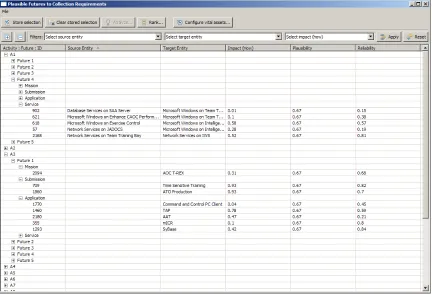
value. Figure 3.3 shows the main window of the tool. Since the plausible futures are stored as rows

in the database it made sense to translate this to the graphical interface as a tree table as well. The

ability to collapse and expand particular activities allows for analysts to focus either on individual

The key features of the decision support tool are: (1) identification of critical futures based on

attributes, (2) allows for analysis of plausible futures based on attributes, and (3) ability to rank of

plausible futures by criteria.

3.1.1 Identification of critical plausible futures

Analysts have insight into assets/entities in a mission which are critical to mission success. Critical

plausible futures are those which have attributes that involve these type of entities. Having these

critical futures emphasized draws an analysts attention and helps them to identify plausible futures.

Thus, the tool allows analysts to configure which assets they consider critical and subsequently

highlights them in the interface.

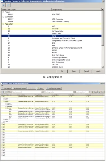
The analyst can configure what attribute (specifically target) they think are critical to the success

of the operation as seen in Figure 3.4a. This results in the plausible futures which involve this

attribute being highlighted in the GUI. This reduces the effort the analyst needs to spend identifying

plausible futures of interest as the number of plausible futures increases. They can spend a minimum

amount of time up front identifying the attributes that they consider vital and allow the tool to

identify the critical plausible futures for them. In implementation, this is accomplished by keeping

a list of vital attributes that are configured by the user in a singleton object. The singleton guarantees

that there is only ever one instance of the list. As the display of the plausible futures occurs each

attribute is checked against the list to determine whether it is critical plausible future or not. Figure

3.4b shows the vital attributes configuration reflected in the main window.

Since the display is tree based, data is also rolled up so that at the highest level the analyst

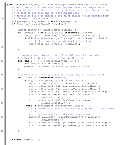
can see vital assets with maximum impact in the display as seen in Figure 3.4b. This functionality

is implemented using the code seen in Figure 3.5. This code recursively traverses the complete

hierarchal tree of all plausible futures in the display and checks to see if each node is one which

involves a critical entity. A RowAggregator object is used to track the maximum values at each

level in the hierarchy. This object stores the current maximum impact value and as the traversal

occurs each node is checked and the maximum value is updated if a new max is found. This results

in the hierarchal rollup which shows the analyst at each level the maximum impact to a critical

asset (Figure 3.4b). The interface draws the analysts attention to certain plausible futures by both

(a) Configuration

(b) Display

1 public static RowAggregator recursivelyUpdateData(TreeItem startingItem) {

// all items in the tree must have children item the length might // just be zero, so this is a safety check to make sure the selection // is part of the tree and not some random item

// default to false to indicate the color should not be changed from

6 // the default background

RowAggregator aggregator = new RowAggregator(); if (startingItem.getItems() != null) {

Object itemData = startingItem.getData();

11 if (itemData != null && itemData instanceof EventRow) { Long curID = ((EventRow) itemData).getTargetEntityID(); if (VitalAssetsManager.getInstance().isVitalAsset(curID)) {

// if this node is a vital asset return true

aggregator.set((EventRow) itemData);

16 }

}

// recurse over the children, if no children the loop stops

TreeItem[] children = startingItem.getItems(); 21 for (int i = 0; i < children.length; i++) {

TreeItem child = children[i];

aggregator.combine(recursivelyUpdateData(child)); }

26 // if there is a max then set the values for it at this point

if (!(itemData instanceof EventRow)) {

if (aggregator.getAggregate().size() == 1) {

EventRow max = aggregator.getAggregate().get(0); startingItem.setText(1, max.getSourceEntityName());

31 startingItem.setText(2, max.getTargetEntityName());

startingItem.setText(3, Double.toString(max.getImpact())); startingItem.setText(4, Double.toString(max

.getPlausibility()));

startingItem.setText(5, Double.toString(max

36 .getReliabililty()));

} else if (aggregator.getAggregate().size() > 1) {

// if there is no max we use a utility method to create some // text

// to reflect this that does not have a max

41 EventRow parsedRow = parseMultiAggregate(aggregator

.getAggregate());

startingItem.setText(1, parsedRow.getSourceEntityName()); startingItem.setText(2, parsedRow.getTargetEntityName()); }

46 }

}

return (aggregator); }

3.1.2 Analysis of plausible futures using attributes

Using the plausible futures tool, the user can also perform analysis for a select set of plausible

futures that they want to consider from the larger overall set. This allows for observations such as

overlaps in attributes between plausible futures. A possible benefit from this is that a single action

might suffice to mitigate the impact of multiple plausible futures if they share attributes.

Figure 3.6a displays the attribute selection screen that is displayed when analysis is performed

on a set of plausible futures. This panel shows all of the attributes related to the selected plausible

futures as well as the activities they belong to. When an analyst looks at the panel they can see which

attributes are shared between plausible futures by the labels beside each attribute. For example, it

can be seen that the target entity attribute‘Microsoft Windows on AOC Weapons System Server’is

involved in two plausible futures (1.5, 3.1). The highlight on‘Network Services on Enhance CAOC

Performance Assessment System Server’denotes that this target entity has previously been marked

as critical by the analyst which helps to draw attention.

The analyst selects attributes they are interested in and can monitor. This brings up a new dialog

as seen in Figure 3.6b, which displays the plausible futures that involve the selected attributes. Rows

highlighted in blue are plausible futures that were part of the initial set selected by the analyst. Gray

highlighted rows are other plausible futures that involve the selected attributes but were not part of

the initial set selected by the analysts. The results pane provides a complete set of plausible futures

that are effectively covered by CRAs performed on the selected attributes.

3.1.3 Ranking plausible futures

A ranking feature was also implemented so that analysts could view the top N ranked plausible

futures based on a specified criteria. The ranking of plausible futures provides another quick way

for analysts to identify important plausible futures. The criteria for the ranking is based on either

subjective assessments or algorithmically. The ranking panel also displays a column which identifies

other plausible futures (that are also ranked or not ranked) that share common attributes with the

ranked plausible future. This allows for analysts to easily identify important CRAs that could cover

multiple plausible futures resulting in more efficient CRAs.

Using the plausible futures tool an analyst can intelligently craft candidate CRAs such as shown

(a) Selection of attributes to compare

(b) Results of analysis

Figure 3.7: Ranking of plausible futures based on attributes

future influences an asset, which implicitly means that an action can be taken to mitigate the impact

from the plausible future.

3.2

Evaluating Mission Impact Using CRA Matrices

As previously state, a current impact matrixand a future impact matrixis used to represent the

state of assets. The current impact matrix is the current state of the assets, and future impact matrix

is the possible state of the assets if plausible futures occur. Actions (candidate actions) can be

       

p1 p2 p3 p4 p5

a1 0 0 0 0 1

a2 0 0 0 1 0

a3 0 1 0 0 0

a4 1 0 1 1 0

a5 1 0 0 1 0

       

      state

a1 0

a2 0

a3 0

a4 0

a5 0

     

(a) Current impact matrix      

p1 p2 p3 p4 p5 a1 0.2 0.0 0.8 0.0 0.64 a2 0.5 0.0 0.0 0.89 0.55 a3 0.0 0.0 0.5 0.26 0.78 a4 0.0 0.98 0.0 0.8 0.0 a5 0.8 0.34 0.0 0.2 0.4

     

(b) Future impact matrix

Figure 3.9: Representing current and future asset states

performed to mitigate the impact from plausible futures, this mitigated impact can be viewed as

the benefit from performing the action. Optimization occurs on the premise of maximizing the

mitigated impact to the mission, not the difference in the states of the assets. The candidate actions

are represented algebraically as CRA matrices as shown in 3.8, which uses a binary value to show

whether a plausible future influences an asset or not.

So in essence, if a CRA is taken (carried out) than the impact from the plausible future is

accounted for and effectively replaces the current impact value in our consideration.

Equation (3.1) selects between the current impact value and a plausible future impact value

(Figure 3.9) based on a decision variable of whether or not a CRA was taken and therefore the impact

was mitigated. A mission model is used to propagate the low level impacts from this evaluation to

the overall mission.

The concept of a mission model has been seen in previous works such as Schubertet al. work

on CIMs and effect-based planning [9, 18, 19]. The framework defines a mission hierarchy (model)

based on an analyst’s expertise as shown in Figure 3.10. The analyst creates the hierarchya priori

to model the relationships and interactions from assets up to the overall mission. The mission

hierarchy defined by the framework does not consider influences by elements at the same level of

the hierarchy. The number of possible combinations of influences as well as their multiplicative

effects are difficult to take into account and thus not within the scope of this work.

The hierarchy is asset based, the assumption is that within any given mission ultimately the

assets allow for the mission to be accomplished by carrying out tasks [12]. The definition of an

asset is purposely loose for generalization purposes. An asset is any entity of value to the mission;

Task 1

+

+ Aggregation function

Task 2

+

Task 3

+

Task 4

+

Asset 1 Asset 2 Asset 3 Asset 4 Asset 5

Mission

+

Figure 3.10: Mission hierarchy tree.

shows an the impact matrices which forms the lowest level of input for the mission hierarchy. Where

the impact values for each asset is a value from [0.0, 1.0] with 1.0 being the maximum impact and

0.0 being no impact. These values are also absolute and not a delta value and can be viewed as the

state of the asset.

3.3

Aggregation Functions

Forward propagation of impacts occurs via aggregation functions such as a weighted average or

Yager’s Ordered Weighted Average [24] [26] [25]. The use of a hierarchy necessitates the use

of functions that can produce representative values from a large number of inputs, aggregation

functions provide this utility. The different levels in a hierarchy can be viewed as progressively

becoming more complex as the number of entities each level encapsulates increases. Aggregation

functions facilitate this representation efficiently and selection of appropriate aggregation functions

to model relationships in a mission is a significant task.

Aggregation functions (operators) are simply functions with special properties [1]:

Definition 3.3.1. An aggregation function is a function of n > 1 arguments that maps the

(i) f(0,0, . . . ,0

| {z }

n times

) = 0andf(1,1, . . . ,1

| {z }

n times ) = 1

(ii) x≤yimpliesf(x)≤f(y)∀x, y∈[0,1]n

3.3.1 Ordered Weighted Average

An aggregation function of particular interest are Ordered Weighted Averages (OWA) [24–26] as

OWA can be used to represent different logical relationships. OWA is exactly the same as a simple

weighted average however the↘subscript indicates that inputs are first sorted in descending order.

This allows OWA to represent different relationships depending on how the weighting vector is

specified. This flexibility is desirable in a model as it simplifies implementation and allows analysts

to create different relationships efficiently.

Definition - Ordered Weighted Average. For a given weighting vector w, wi ≥ 0,∑wi = 1, the OWA function [1, 24] is given by

• OW Aw(x) = n

∑

i=1

wix(i)=⟨w,x↘⟩

wmax =

[

1 0 0 0 0

]

x_↘=

[

5 4 3 2 1

]

wtop2=

[

0.5 0.5 0 0 0

]

x_↘=

[

5 4 3 2 1

]

Since OWA can be used to formulate different relationships analysts can change the weights of

the function as parameters rather than using explicit logical functions.

3.4

Optimization Formulation

The final step in the framework is the ability to optimize the set of CRAs to select the best based on

Equation 3.3 defines a cost constraint which limits the amount of feasible CRAs that can be

taken based on resources available. Equation 3.4 is a timing constraint that limits which CRAs can

be taken based on turnaround time.

Variables

X(n) =

    

1, If CRAnis selected

0, o.w.

Amax(j) =whether plausible future j has maximum impact

Tmax(i) =whether asset i has maximum impact

Mmax(l) =whether task l has maximum impact

α(i, j) =

    

1, assetifor plausible futurejis monitored

0, o.w.

y(i) =aggregated impact on asseti

Dtask(l) =aggregated impact on taskl

Dm =aggregated impact on mission

Parameters

cn=cost of executingXn

tn=time alotted forXnto complete

T =max turnaround time

B =total budget

An(i, j) =monitored stated for asseti, plausible futurej

Sc(i) =current impact for asseti

Sf(i, j) =future impact for asseti, plausible futurej

Objective:

Subject to:

n

∑

i=1

Xn·ci ≤B (3.3)

Xn·tn≤T,∀n (3.4)

α(i, j)≥Xn·CRAn(i, j),∀i, j, n (3.5)

α(i, j)≤ n

∑

i=1

Xn·CRAn(i, j),∀i, j (3.6)

y(i) =maxj(Sf(i, j)α(i, j))

+Sc(i)(1−maxj(α(i, j))),∀i, j

(3.7)

i

∑

k=1

Tmax=i−1 (3.8)

y(i)≤Dtask(l),∀i, l (3.9)

Dtask(l)≤C·Tmax(l, i) +y(i),∀i, l (3.10)

l

∑

k=1

Mmax=l−1 (3.11)

Dtask(l)≤Dm,∀l, m (3.12)

Dm ≤C·Mmax(l) +Dtask(l),∀l, m (3.13)

The optimization formulation incorporates all of the ideas previously mentioned.

3.4.1 Logical Constraints

Logical constraints need to be algebraically formulated to be used in MIP solvers such as Gurobi.

j

∑

k=1

Amax=j−1 (3.14)

y(i, j)≤Dasset(i) (3.15)

Dasset(i)≤C·Amax(i, j) +y(i, j) (3.16)

Constraints 3.14, 3.15, 3.16 enforce a max relationship as the aggregation function for asset

damage. The following example illustrates the logic which create the max relationship.

IfAmaxis a matrix of binary decision variables (i.e.,values are bounded from 0 to 1).

A=

[

0 1 1 1 1

]

y(i, j) =

[

4 3 5 1 2

]

IfAhas a value of zero corresponding with four iny(i, j)then 3.15 is violated since 3.16 forces

Dassetto be four. In fact for all values except five this constraint is violated. WhenAhas a value

of zero corresponding with five, Dasset is bounded on top to be 5 and it is indeed greater than or

equal to all other elements which satisfies constraint 3.15. The constantCis just a sufficiently large

constant that should be much greater than all values iny(i, j). Since the values in the impact matrix

fall between zero and one, a value of one can be used as the constant. Due to computation concerns

the smallest value constant possible should always be used based on analysis of the inputs.

A logical mininum constraint can be constructed in a similar fashion by putting the binary

variable (in 3.16) to the lower bound and changing the addition to subtraction. So that the constraint

forces the minimum value to fixed only when.

j

∑

k=1

Amin =j−1 (3.17)

Dasset(i)≤y(i, j) (3.18)

// Constraint that ensures only one element in aMax // will be zero and all others are 1

//

// : sum(aMax_j) == n - 1

5 for (int i = 0; i < numAssets; i++) {

GRBLinExpr exprLHS = new GRBLinExpr(); for (int j = 0; j < numFutures; j++) {

exprLHS.addTerm(1.0, aMax[i][j]); }

10 model.addConstr(exprLHS, GRB.EQUAL, numFutures - 1, ""); }

// Ensures that the assetImpact is bounded on the bottom

for (int i = 0; i < numAssets; i++) {

15 GRBLinExpr exprRHS = new GRBLinExpr(); exprRHS.addTerm(1.0, assetImpact[i]);

for (int j = 0; j < numFutures; j++) {

GRBLinExpr exprLHS = new GRBLinExpr();

20 exprLHS.addTerm(1.0, y[i][j]);

model.addConstr(exprLHS, GRB.LESS_EQUAL, exprRHS, ""); }

} 25

// Ensures that the assetImpact is bounded from the top

for (int i = 0; i < numAssets; i++) {

GRBLinExpr exprLHS = new GRBLinExpr(); exprLHS.addTerm(1.0, assetImpact[i]); 30

for (int j = 0; j < numFutures; j++) {

GRBLinExpr exprRHS = new GRBLinExpr(); exprRHS.addTerm(1.0, y[i][j]);

exprRHS.addTerm(1000, aMax[i][j]);

35 model.addConstr(exprLHS, GRB.LESS_EQUAL, exprRHS, ""); }

}

Figure 3.11 shows how logical constraints (in this case max) can be written in Gurobi. The

figure shows that writing constraints in a modeling package requires the use of for loops to replicate

the∀(i, j) condition. The model is represented as a single object and all variables are for defined

for this model. The model is solved via amodel.optimize()method call.

3.5

Implementation of Optimization Problem

After the set of CRAs have been determined and the mission hierarchy used to evaluate how these

CRAs impact the overall mission. The next logical step is to optimize and select a subset of the

CRAs based on the tradeoff of feasibility and cost-effectiveness. This problem was formulated as

a mixed integer programming problem based on the requirements of the inputs: the selection of

CRAs is binary and the evaluation of mission impact values is continuous.

There are many different optimization packages available for MIP problems. However, in

im-plementation the most important step is to start at the algebraic formulation to determine the

require-ments needed from the package chosen. From Chapter 3.4 the requirerequire-ments are that the package can

solve MIP type problems, and be able to handle a large number of constraints. The most well known

commercial solvers were considered: Lindo, CPLEX, Microsoft Solver Foundation. The problem

with selecting these packages are that they are expensive. Gurobi is a recently released optimization

package that is available commercially but also offers free academic licenses. These packages each

have different interfaces for creating the model. Lindo uses a modeling language called LINGO,

and CPLEX can be used with OPL. The modeling languages closely reflect algebraic formulations

and simplify the implementation of algebraic expressions. Alternatively, all packages have s which

allows for standard programming with languages such as Java, C++_{, C}#_{, and Python. Gurobi was}

selected as the package of choice due to easy access. Microsoft Excel also includes a Solver which

was used a simple alternative used for prototyping and smaller problems.

Algorithm 1Gurobi optimization problem setup create parameter matrices

model.create()

create and add decision variables to model define constraints

Figure 1 presents the basic flow for setting up an optimization problem in Gurobi. These

Chapter 4

Case Study

A case study was performed to evaluate the frame work. The case study emulated the processes an

analyst would perform using the framework to demonstrate its capabilities.

4.1

Scenario: Hostage Rescue

A hostage rescue scenario was considered involving a special forces team sent to rescue hostages

being held by a terrorist group. A helicopter is to be used for transporting the team and extracting

the team and rescued hostages.

Mission

A special forces team is sent to rescue a group of hostages being held by

terror-ists. The operation uses a helicopter for transport.

In planning the mission an analyst can anticipate the the following plausible futures.

Plausible Futures

The terrorists could acquire weapons to use against the special forces team (p1)

Terrorist scouts perform surveillance on friendly forces (p2)

Terrorist combatants utilize their intelligence on friendlies to lay an ambush (p3)

The terrorists decide to relocate the hostages (p4)

The terrorists decide execute the hostages (p5)

From the friendly analyst’s perspective the following assets are of interest to the overall mission

ID Plausible Future Source Target Impact

1 Acquire weapons Terrorists leadership Special forces 0.9

2 Acquire weapons Terrorists leadership Hostages 0.6

3 Acquire weapons Terrorists leadership Helicopter 0.8

4 Acquire weapons Terrorists leadership Landing site 0.55

5 Acquire weapons Terrorists leadership Friendly base 0.6

6 Surveillance Terrorist scouts Special forces 0.7

7 Surveillance Terrorists scouts Hostages 0.2

8 Surveillance Terrorists scouts Helicopter 0.55

9 Surveillance Terrorists scouts Landing site 0.75

. . . . .

. . . . .

. . . . .

(a) Plausible futures

ID Attribute name

1 Special forces

2 Hostages

3 Helicopter

4 Landing site

5 Friendly base

(b) Assets

Figure 4.1: Attribute-based analysis of plausible futures

Assets

Special forces team (a1)

Hostages (a2)

Helicopter (a3)

Landing site for helicopter (a4)

Friendly base (a5)

Finally, a set of tasks need to be accomplished to successfully complete the hostage rescue.

Tasks

Land safely in drop off zone (t1)

Secure terrorist base (t2)

Capture terrorists (t3)

Rescue hostages (t4)

Return to base (t5)

An analyst can arrive at estimated impacts of plausible futures to assets. These estimates can be

derived from an analyst’s experience, intuition, and with the aid of automated tools.

Figure 4.2 shows the estimated future impacts from plausible futures. An analyst can arrive at

       

Acquire weapons Surveillance Ambush Relocate Execute

Special forces 0.9 0.7 0.85 0.6 0.3

Hostages 0.6 0.2 0.5 0.7 1

Helicopter 0.8 0.55 0.8 0.1 0.05

Landing site 0.55 0.75 0.9 0.15 0.05

Friendly base 0.6 0.5 0.2 0.3 0.05

       

Figure 4.2: Future impact matrix

     

p1 p2 p3 p4 p5

a1 0 0 0 0 0

a2 0 0 0 1 1

a3 0 0 0 0 0

a4 0 0 0 0 0

a5 0 0 0 0 0

      (a)      

p1 p2 p3 p4 p5

a1 1 0 0 0 0

a2 1 0 0 0 0

a3 1 0 0 0 0

a4 0 0 0 0 0

a5 0 0 0 0 0

      (b)      

p1 p2 p3 p4 p5

a1 0 1 0 0 0

a2 0 0 0 0 0

a3 0 0 0 0 0

a4 0 1 0 0 0

a5 0 1 0 0 0

      (c)      

p1 p2 p3 p4 p5

a1 0 0 0 1 0

a2 0 0 0 1 0

a3 0 0 0 0 0

a4 0 0 0 1 0

a5 0 0 0 0 0

      (d)      

p1 p2 p3 p4 p5

a1 0 0 1 0 0

a2 0 0 0 0 0

a3 0 0 1 0 0

a4 0 0 1 0 0

a5 0 0 0 0 0

      (e)

An analyst must then consider a set of collection requirement actions that are derived from

the plausible futures. The developed plausible futures tool facilitates this process. Figure 4.1(a)

shows example plausible futures as well as their corresponding attributes. From the analysts point

of view the friendly assets would be critical to mission success. Analysis can be performed using

the plausible futures tool. If the analyst selects the special forces team and hostages as vital to the

mission. The result would be that the analyst’s attention would be drawn to the plausible futures

which involve these assets. The analyst notice that one of the highest impact plausible futures (i.e.,

terrorists acquire weapons) involves this asset so a CRA that monitors this plausible future would

be advisable.

The collection requirement (CRA 1) that is derived is that the weapons capability of the terrorists

must be monitored. Appropriate actions must be defined by the analyst to determine what weapons

the adversary has access to. A subjective relative cost is assigned to the CRA of 0.5 (with a range

of 0 to 1.0). To differentiate between the different CRAs so cost and time required for each CRA

can be assigned relative to each other. Figure 4.3(a) shows the matrix representation of this CRA.

The values in the matrix reflect the analyst’s intuition regarding which assets could be influenced if

this collection requirement is selected. In this case if the weapons capability of the terrorists is not

determined the weapons could in turn be used against the special forces team, the helicopter, and

possibly hostages. For simplification the time required for all CRAs to be performed in the case

study was set at relative value of 0.5 units. The timing constraint in this case study is used limit

feasible number of actions.

A second CRA (CRA 2) would be to determine the state of the hostages. An analyst can expect

that the terrorists would communicate and give demands which would mean determining this

infor-mation is relatively low cost so a value of 0.10 can be subjectively assigned. Figure 4.3(b) shows

the matrix representation of this CRA. Intuitively if the hostages are executed or relocated then they

would be impacted, the matrix reflects this idea.

The analyst would likely also want to know about the terrorist’s intelligence level on friendlies.

This forms the third CRA (CRA 3) as shown Figure 4.3(c). Due to the complexity of determining

such information the cost of this CRA is rated high relative to the others at 0.75. The matrix shows

that if surveillance has occurred it would likely impact the friendly base as well, special forces team,

Collection requirements could also be related to each other. For example, if the terrorists have

adequate intelligence on friendly forces they might choose to relocate the hostages. This would

require a new CRA (CRA 4) to determine the location of the hostages. Since the operational areas

of the terrorists can be determined from previous