Classification of ordered texture images using regression modelling and granulometric features

(1)

Classification of Ordered Texture Images using

Regression Modelling and Granulometric Features

Mahmuda Khatun

Department of Mathematics

and Statistics University of Strathclyde

Glasgow, UK G1 1XH Email: [email protected]

Alison Gray

Department of Mathematics

and Statistics University of Strathclyde

Glasgow, UK G1 1XH Email: [email protected]

Stephen Marshall

Department of Electronic and Electrical Engineering

University of Strathclyde Glasgow, UK G1 1XW Email: [email protected]

Abstract—Structural information available from the

granu-lometry of an image has been used widely in image texture analysis and classification. In this paper we present a method for classifying texture images which follow an intrinsic ordering of textures, using polynomial regression to express granulometric moments as a function of class label. Separate models are built for each individual moment and combined for back-prediction of the class label of a new image. The methodology was developed on synthetic images of evolving textures and tested using real images of 8 different grades of cut-tear-curl black tea leaves. For comparison, grey level co-occurrence (GLCM) based features were also computed, and both feature types were used in a range of classifiers including the regression approach. Experimental results demonstrate the superiority of the granulometric moments over GLCM-based features for classifying these tea images.

Index Terms—Granulometry, pattern spectrum, structuring

element, ordered texture, tea granule images

I. INTRODUCTION

Many methodologies have been proposed to determine the physical/chemical properties of foods, using chemometrics, pattern recognition and/or image analysis techniques, e.g. [1]– [8]. Applications of digital image processing techniques are expanding rapidly in the food processing industries.

Here we investigate the advantages of granulometric mo-ments over GLCM-based features for classifying 8 different grades of tea images. Granulometries extract shape-based textural information, hence are useful for analysing and classi-fying shape-based images. Originally developed by Matheron [9] in the binary case to characterise the size and shape information of a random set, the granulometric approach was extended to the grey scale case by many others, e.g. [10]– [14]. It has been used extensively in texture analysis and classification. For example, granulometric moments were used to characterise evolution of a dynamic process concerning paint drying in [15]. Binary images of the corneal endothelium were classified as normal or pathological cases in [16] using the granulometric size distribution of the images. The first two granulometric moments were used to classify white blood cells in bone marrow images in [17]. Evolving texture images of corrosion were classified using granulometric moments by means of a parallel evolution function in [18]. A combination of opening granulometry and closing granulometry was

em-ployed in [19] to classify grey scale Brodatz texture images [20].

GLCM is a statistical approach to texture classification which characterises the spatial relationships between the grey levels of pixels, and has proved useful in various texture classification applications because of its ability to extract spatial information. GLCM features were used in a self-organising map in [21] to classify Brodatz texture images with 97% classification accuracy. GLCM features and linear discriminant analysis (LDA) were successfully used to classify colour images of colon cancer in [22]. These features were also found to be useful for classifying colour texture images in [23].

In this work, we consider ordered textures. We define ordered textures as those which can be ranked according to some scale of fineness or coarseness, or by size of texture primitives (shapes) in the images. Building on [18], we de-velop a regression-based classifier by modelling granulometric moments or GLCM features as a function of texture class label. A cubic polynomial regression is fitted for each chosen feature separately, and then a combined cubic polynomial regression is obtained for back-prediction of the class label of a new image using its observed features. Several classifiers, i.e. a support vector machine (SVM), LDA, a feed-forward neural network (FF-NNET) and the regression classifier were employed using the same sets of features to compare their relative classification accuracy.

For testing, we use a sequence of cut-tear-curl (CTC) black tea images (Figure 1) representing 8 different grades of tea of different granule sizes as used in [5]. The images were sorted visually according to their granule size and were labelled as class 1 to 8, from the smallest to the largest granule size, so that the tea granules increase in size between the classes. The next section briefly describes the methods used in [5], with some other work relating to tea images.

A. Related work

(2)

have investigated texture analysis and classification techniques to develop a more automated approach. Some recent work is summarised here.

Indian CTC black tea granules comprising eight grades of tea from different tea gardens in Assam, India were classi-fied according to granule size in [5]. Four-level pyramidal decomposition using Daubechies wavelets was applied to each grey scale image. Initially, energy and entropy from each of four approximation sub-bands were used as features in principal component analysis (PCA) and the self-organising map (SOM) clustering technique, however these were unable to clearly separate the grades. A pair of most similar images from each grade were identified using Mahalanobis distance of their feature vectors, and one of these images was selected as a typical image from that grade. New features were calculated as the Mahalanobis distance of a given image to the chosen typical image in each grade. With the new distance features, PCA and SOM were able to distinguish the grades better. Two different neural networks, a multi-layer perception (MLP) and learning vector quantisation (LVQ), were trained using

700 images and tested on another 150images, and achieved

74.67%and 80%classification accuracy respectively. In this paper, we apply our methodology to some of these same images below, with much improved results.

Hyperspectral images of five grades of roasted green tea leaves were classified in [4]. Four texture descriptors, namely mean, sd, energy and entropy, were computed from 3 optimum waveband images (chosen by PCA), and used as features in a SVM, with 95%correct classification. In [7], six different classes of tea were used. The discrete cosine transform was used on multi-spectral images (red, near-infrared (NIR) and green bands). Using the standard deviation (sd) of each of the original or filtered NIR images with a SVM produced 73.33% or 100% correct classification respectively. Five dif-ferent grades of Chinese green tea brands were classified using multi-spectral colour images in [8]. GLCM features computed from wavelet decomposition of each of the three image colour planes were used with LDA, giving 100% accurate classification. Four different categories of Chinese green tea were distinguished using entropy values calculated from multi-spectral images in [6]. A least squares support vector machine produced 97.5% to 100% classification accuracy.

II. METHODOLOGY

Texture classification involves a step to extract features from the image under study, and a classification step, in which a texture class membership is assigned to the image, based on information provided by the extracted texture features through appropriate machine learning algorithms [24]. This section describes the feature extraction techniques and classifiers used in this work.

A. Opening granulometry

As a texture image can be considered as a collection of grains [13], the concept of opening granulometry is to sieve the grains through filters of increasing size, so that grains

with size smaller than the sieve mesh drop out and only grains with larger sizes remain. The shape of the holes is determined by the shape of the structuring element (SE), which is a geometrical pattern used to extract textural infor-mation from a given digital image [25]. That is, if image f is opened sequentially by a series of SEs of increasing size,

{g1, g2, . . . , gN}, at each stage of opening the finer details

will successively be eliminated and the volume (sum of pixel intensities) of the input image will reduce eventually to zero, i.e. Ω(1) ≥ Ω(2) ≥ . . . ≥ Ω(N), where Ω(j) is the image volume left after thejth_{opening. This decreasing sequence is}

called the size distribution [13].

Normalising the size distribution asΦ(n) = 1−Ω(n)/Ω(0), where Ω(0) is the original image volume, gives a cumu-lative distribution function (cdf) which rises monotonically from 0 to 1 as the size of the SE increases. Its derivative

Φ′₍_n_{) =} _d_Φ(_n₎_/dn _{is a probability density function (pdf),} referred to as the pattern spectrum (PS) [26]. As a pdf, this can be summarised by its statistical moments. In the discrete case, the scaling factor n is an integer, so the mth _{granulometric}

moment may be calculated as

µm= N X

n=1

nmΦ′(n).

We use these moments to compute the mean µ = µ1,

standard deviation (sd) σ = √ν2, skewness and (excess)

kurtosis ofΦ′(n), calculated from the central momentsνm= PN

n=1(n−µ1)mΦ′(n). The skewness is ν3/σ3, and kurtosis

isν4/σ4−3. We refer to these four moments below as the PS

moments. These moments contain useful textural information to characterise the texture images.

B. Grey level co-occurrence matrix (GLCM)

The GLCM is a G×G matrix where Gis the number of grey levels in the original image. The entryC(i, j)of a GLCM is the frequency of grey levelsiandj of pixels separated by inter-pixel distance d and lying on a line at angle φ to the reference direction of the image. To reduce the sparsity of the GLCM, the original image is often quantised first to some lower level, e.g. 8, 32, or 64 [27]. The normalised GLCM p(i, j)can be obtained by dividing C(i, j) by the sum of its entries as

p(i, j) =C(i, j)/

G X

k=1

G X

l=1

C(k, l),

whereGis the number of grey levels after any quantisation. Haralick et al. [28] proposed extracting some features from the GLCM for more compact texture representation, including:

1) Maximum probability :max(i,j)p(i, j)

2) Energy :PG i=1

PG

j=1p(i, j)2

3) Entropy : -PG i=1

PG

j=1p(i, j) logp(i, j)

4) Contrast:PG i=1

PG

j=1(i−j)2p(i, j)

5) Homogeneity:PG i=1

PG j=1

p(i,j)

(3)

6) Correlation : _σ1

iσj

PG i=1

PG

j=1(i−µi)(j −µj)p(i, j),

where µi =P

G i=1i

PG

j=1p(i, j), µj =P G i=1j

PG

j=1p(i, j),

σ2

i = PG

i=1(i−µi)2

PG

j=1p(i, j),andσ2j = PG

j=1(j−

µj)2PG

i=1p(i, j).

We also use these below as texture features for classification.

C. Classifiers

Let Yi(c), i = 1,2, . . . , p, and c = 1,2, . . . , K be the average value of the ith _{feature for the images in the} _cth

class. A regression classifier is built by modelling each average feature separately as a function of class label using a cubic polynomial regression model, written as:

Yi(c) =β0(i)+β

(i)

1 ∗c+β

(i)

2 ∗c2+β

(i)

3 ∗c3+ξi, (1)

where the parametersβterms are estimated using least squares and the ξi are error terms.

For a single feature ithe model is of the form:



  

Yi(1)

Yi(2)

. ..

Yi(K)

    =     

β₀(i)+β₁(i)c1+β₂(i)c21+β(

i₎

3 c31 β₀(i)+β₁(i)c2+β₂(i)c22+β(

i₎

3 c32

.. .

β(₀i)+β₁(i)cK+β( i₎

2 c2K+β

(i₎

3 c3K

     +     ε1 ε2 . .. εK     .

Forpsuch features, a combined fitted model relating each feature to class is formed as:

     ˆ

Y1(c)

ˆ

Y2(c)

.. .

ˆ

Yp(c)      =       ˆ

β₀(1)+ ˆβ(1)₁ c+ ˆβ₂(1)c2_{+ ˆ}_β(1)

3 c3

ˆ

β₀(2)+ ˆβ(2)₁ c+ ˆβ₂(2)c2_{+ ˆ}_β(2)

3 c3

.. .

ˆ

β(0p)+ ˆβ

(p)

1 c+ ˆβ

(p)

2 c2+ ˆβ

(p)

3 c3

      , (2)

or Yˆ _{= ˆ}BC, where

ˆ B₌       ˆ

β0(1) βˆ (1)

1 βˆ

(1)

2 βˆ

(1) 3

ˆ

β0(2) βˆ (2)

1 βˆ

(2)

2 βˆ

(2) 3

..

. ... ... ...

ˆ

β₀(p) βˆ₁(p) βˆ(₂p) βˆ₃(p)

     

is ap×4matrix andC_{= [1}_{, c, c}2_{, c}3_]′is a4×1vector. This combined model is used for prediction.

The above can be re-written as

     ˆ

Y1(c)

ˆ

Y2(c)

.. .

ˆ

Yp(c)      −       ˆ

β₀(1)

ˆ

β₀(2) .. .

ˆ

β(₀p)

      =       ˆ

β₁(1) βˆ₂(1) βˆ₃(1)

ˆ

β₁(2) βˆ₂(2) βˆ₃(2) ..

. ... ...

ˆ

β₁(p) βˆ₂(p) βˆ₃(p)

        c c2 c3  ,

or, using matrix notation, as:

_ˆ

Y₋βˆ₀ = _ˆ

β₁ βˆ₂ βˆ₃

  c c2 c3 

. (3)

Pre-multiplying by(Yˆ ₋βˆ₀)′ _gives

(Yˆ₋βˆ₀)′(Yˆ₋βˆ₀) = (Yˆ₋βˆ₀)′ _ˆ

β₁ βˆ₂ βˆ₃

  c c2 c3  ,

a cubic equation incof the formA1c3+A2c2+A3c+A4= 0.

A positive real root of this equation is used as the predicted class c. Where there is more than one positive real root we choose the smallest one (as was appropriate in all our training examples). If none of the roots are positive and real the method fails to predict the class, and we choose the first class as the prediction.

We employed SVM, LDA and FF-NNET as benchmark methods to compare the performance of this regression ap-proach.

Developed by Vapnik and Cortes [29], SVM is a very powerful classification technique, which is robust in producing high classification accuracy even in high-dimensional data spaces with non-linearly separable classes [30]. Its theoret-ical foundation is based on the structural risk minimisation principle [31]. We used the one-to-one classification approach for this multiple class problem, and tuned the choice of kernel, any associated kernel parameter values and the cost parameter used, in the SVM training for optimum classification results. We also used LDA, which assigns a new feature vector to the class with maximum posterior probability, assuming normality of the class conditional distributions and a common within-class feature covariance matrix [32]. A FF-NNET with single hidden layer is also used [30], with the number of neurons in the hidden layer optimised in training. The R software package was used for SVM, LDA and FF-NNET with libraries e1071,

MASS and nnet respectively.

The prediction abilities of the classifiers are assessed using misclassification rate and mean absolute error (MAE), defined as:

MAE = 1

n

n X

i=1

|ti

pred−tiact|, (4)

where n is the number of images for which the class is to be predicted, andti

pred andtiact are respectively the predicted

class label (rounded if necessary) and the actual class label of imagei.

III. APPLICATION TO TEA IMAGES

A. Data description

(4)

diameters in mm of the granules are 2.0, 1.7, 1.3, 1.0, 0.5,

0.355,0.25and Not specific respectively [5].

We obtained training and test sets by extracting 2562 _size

images from each of the original images and converted them to grey scale. Fifty non-overlapping sub-images were extracted from one image from each class, giving a total of400sample images. One sub-image from each class is shown in Figure 1, to show the progression in size of the tea granules over the classes.

(a) Class 1 (b) Class 2 (c) Class 3 (d) Class 4

[image:4.612.320.555.53.259.2]

(e) Class 5 (f) Class 6 (g) Class 7 (h) Class 8

Fig. 1: Sample grey scale tea images of size 2562_{, one from}

each of the eight tea classes.

B. Feature extraction

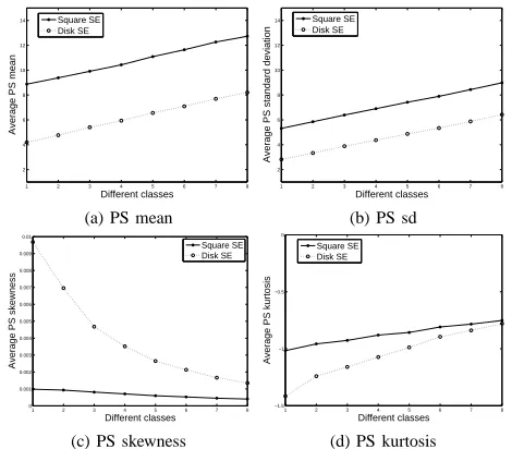
There exists substantial variation of intensity within images. To improve this, top-hat transformation was applied as a pre-processing step in order to suppress dark parts and highlight bright parts of the images. Since granule size increases over classes, a disk SE of increasing size is used in the top-hat transformation. Then we applied granulometry using a square and a disk SE and computed the first four PS moments of the pattern spectrum from each SE. Average PS moments are obtained using all sub-images from each class and are plotted against class in Figure 2. The PS mean and sd using all SEs increase with class, while skewness decreases, though for the disk SE the decrease is very slow. Kurtosis for both square and disk SEs is negative and increases slightly with class.

These PS moments are then used as texture features for predicting the class of a tea image. We implemented the regression approach (REG), SVM, neural network and LDA as classifiers and compared their efficiency.

We then computed the six different GLCM features in Section II from each of the 50 sub-images from each class at quantisation level 8 for four different orientations and separation 1, and averaged these over all sub-images. The average features are plotted against class in Figure 3. Entropy and correlation increase with class. Maximum probability and energy decrease with class, but no trend is clear for contrast or homogeneity as a function of class.

1 2 3 4 5 6 7 8

2 4 6 8 10 12 14

Different classes

Average PS mean

Square SE Disk SE

(a) PS mean

1 2 3 4 5 6 7 8

2 4 6 8 10 12 14

Different classes

Average PS standard deviation

Square SE Disk SE

(b) PS sd

1 2 3 4 5 6 7 8

0 0.001 0.002 0.003 0.004 0.005 0.006 0.007 0.008 0.009 0.01

Different classes

Average PS skewness

Square SE Disk SE

(c) PS skewness

1 2 3 4 5 6 7 8

−1.5 −1 −0.5 0

Different classes

Average PS kurtosis

Square SE Disk SE

[image:4.612.55.294.183.322.2]

(d) PS kurtosis

Fig. 2: Average PS moments, of all50top-hat sub-images from each class, plotted against class, for square and disk SEs.

1 2 3 4 5 6 7 8

2.1 2.15 2.2 2.25 2.3 2.35 2.4 2.45 2.5

Different classes Average Entropy _{0 degree}

45 degree 90 degree 135 degree

(a) Average Entropy

1 2 3 4 5 6 7 8

0.19 0.2 0.21 0.22 0.23 0.24 0.25 0.26 0.27 0.28

Different classes

Average Maximum Probability

0 degree 45 degree 90 degree 135 degree

(b) Average Maximum Probability

1 2 3 4 5 6 7 8

0.24 0.26 0.28 0.3 0.32 0.34 0.36 0.38 0.4 0.42 0.44

Different classes

Average Contrast

(c) Average Contrast

1 2 3 4 5 6 7 8

0.78 0.8 0.82 0.84 0.86 0.88 0.9 0.92

Different classes Average Correlation 0 degree

45 degree 90 degree 135 degree

(d) Average Correlation

1 2 3 4 5 6 7 8

0.11 0.12 0.13 0.14 0.15 0.16 0.17

Different classes

Average Energy

(e) Average Energy

1 2 3 4 5 6 7 8

0.8 0.81 0.82 0.83 0.84 0.85 0.86 0.87 0.88

Different classes

Average Homogeneity

(f) Average Homogeneity

Fig. 3: Average GLCM features against class for the grey scale tea images, using quantisation level 8, a single inter-pixel distance and four orientations (0◦_,₉₀◦_,₄₅◦ _and₁₃₅◦_).

IV. EXPERIMENTAL RESULTS

A. Results for PS moments

[image:4.612.322.554.300.607.2]

(5)

classifiers to classify the tea images according to granule size. For all classifiers, 70% of the sub-images from each class were randomly chosen as a training set and the remaining 30% sub-images were used as a test set. The process was repeated 10 times and the results were averaged over the 10 runs.

Table I shows that the SVM attained 100% correct classi-fication using the 4 PS moments computed from a disk SE, or a square SE, or both (using a linear kernel and cost of 1 or more for optimal results). The other classifiers produce lower error rates using the PS moments from the disk SE than the square SE. We also investigated using the moments from both the square and disk SEs, which gives similar results to the disk SE. (FF-NNET used 4, 10 and 10 hidden neurons respectively in the cases of the square SE, disk SE and both). Selection of an optimal SE depends on the geometric shapes we attempt to extract from the image. Tea granules are more likely to be a disk shape than square, so we would expect better classification using a disk SE.

TABLE I: Overall proportion of test images misclassified by all classifiers, using different sets of PS moments.

SE REG SVM LDA FF-NNET

Square 0.214 0 0.018 0.019

Disk 0.123 0 0.009 0.012

Square+Disk 0.129 0 0.003 0.008

[image:5.612.353.524.219.424.2]

Therefore we computed class-wise proportions of images misclassified, and MAE as in (4), for all classifiers using the 4 PS moments from the disk SE (Table II). The proportions misclassified and the MAEs are identical, as the predicted classes are at most one unit away from the actual class results. The SVM classifies perfectly, LDA is next best (a 0.9% error rate), then FF-NNET (1.3% error rate), and then REG with a 9.9% error rate.

TABLE II: Class-wise and overall proportion of test images misclassified for all classifiers using 4 PS moments from a disk SE.

Class Proportion misclassified

REG SVM LDA FF-NNET

1 0.000 0 0.000 0.000

2 0.000 0 0.000 0.000

3 0.020 0 0.000 0.000

4 0.000 0 0.000 0.000

5 0.100 0 0.000 0.000

6 0.160 0 0.000 0.020

7 0.220 0 0.030 0.046

8 0.290 0 0.040 0.033

Overall 0.099 0 0.009 0.013

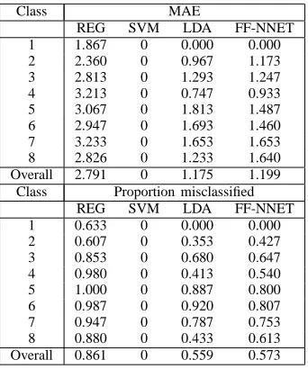
B. Results for GLCM-based features

We also used 4 GLCM features, i.e. entropy, maximum probability, correlation and energy, computed at quantisation 8 and 135◦ _{orientation for classification. The same training} strategy as above was applied for all classifiers (resulting in 8 hidden neurons in FF-NNET, and a linear SVM kernel with a

cost of 1 or higher giving best results). Results are listed in Table III.

The MAE and proportion of test images misclassified are different in this case, as some of the predicted classes are more than one unit away from the actual classes. REG produced the highest MAE, and SVM the lowest. Again SVM is best, with no classification error, compared to 86.1%, 55.9% and 57.3% error rates respectively for REG, LDA and FF-NET. All except SVM are much poorer using the GLCM features than using the PS moments.

TABLE III: MAE and proportion of test images misclassified for all classifiers using 4 GLCM features.

Class MAE

REG SVM LDA FF-NNET

1 1.867 0 0.000 0.000

2 2.360 0 0.967 1.173

3 2.813 0 1.293 1.247

4 3.213 0 0.747 0.933

5 3.067 0 1.813 1.487

6 2.947 0 1.693 1.460

7 3.233 0 1.653 1.653

8 2.826 0 1.233 1.640

Overall 2.791 0 1.175 1.199

Class Proportion misclassified

REG SVM LDA FF-NNET

1 0.633 0 0.000 0.000

2 0.607 0 0.353 0.427

3 0.853 0 0.680 0.647

4 0.980 0 0.413 0.540

5 1.000 0 0.887 0.800

6 0.987 0 0.920 0.807

7 0.947 0 0.787 0.753

8 0.880 0 0.433 0.613

Overall 0.861 0 0.559 0.573

V. SUMMARY AND CONCLUSIONS

This work provides greatly improved results of classifying these tea images compared to the results of [5], for all of the classifiers used. Our highest misclassification rate was for the regression approach (9.9%), and the lowest was 0% for the SVM, using PS moments from the top-hat transformed images, whereas the error rates in [5] for the MLP and LVQ classifiers are25.33%and20%respectively. Their results are not exactly comparable to ours, as we have extracted our own sub-images for algorithm development and testing. Nonetheless we conclude that extracting shape-based information from the tea granule images directly by use of morphological techniques provides very useful features for texture classification in any of a range of classifiers.

[image:5.612.89.261.524.627.2]

(6)

respectively, whereas using increasing disk size in the top-hat transformation most of these classifiers achieved perfect or near perfect classification accuracy.

PS moments provide much better classification than GLCM features for these images. It was also found that a higher level of quantisation does not guarantee better classification results [27], as GLCM features computed at quantisation level 64 produced higher error rates for all classifiers except SVM.

ACKNOWLEDGMENTS

We are very grateful to E. Hines, S. Borah and M. Bhuyan for access to, and use of, the black tea granule images. Mah-muda Khatun was supported by a University of Strathclyde scholarship which made this work possible.

REFERENCES

[1] M.S. Zenoozian and S. Devahastin, Application of wavelet transform

coupled with artificial neural network for predicting physicochemical properties of osmotically dehydrated pumpkin, Journal of Food

Engineer-ing, 90(2) (2009) 219-227.

[2] N. Bhattacharyya, S. Seth, B. Tudu, P. Tamuly, A. Jana, D. Ggosh, R. Bandyopadhyay, M. Bhuyan and S. Sabhapandit, Detection of optimum

fermentation time for black tea manufacturing using electronic nose,

Sensors and Actuators B, 122 (2007) 627-634.

[3] S. Borah and M. Bhuyan, Non-destructive testing of tea fermentation

using image processing, Journal of Insight, 45 (2003) 55-58.

[4] J. Zhao, Q. Chen, J. Cai and Q. Quyang, Automated tea quality

clas-sification by hyper-spectral imaging, Journal of Applied Optics, 48(19)

(2009) 3557-3564.

[5] S. Borah, E.L. Hines and M. Bhuyan, Wavelet transform based image

texture analysis for size estimation applied to the sorting of tea granules,

Journal of Food Engineering, 79(2) (2007) 629-639.

[6] W. Di, H. Yang, X. Chen, Y. He and X. Li, Application of image texture

for the sorting of tea categories using multi-spectral imaging technique and support vector machine, Journal of Food Engineering, 88(4) (2008)

474-483.

[7] X-J. Chen, H-Q. Yang, D. Wu and Y. He, A new method to discriminate

tea categories, Proceedings of the 7th World Congress on Intelligent

Control and Automation, Chongqing, China, (2008) 2236 - 2240. [8] X-L. Li, Y. He and Z-j. Qiu, Textural feature extraction and optimization

wavelet sub-bands for discrimination of green tea brands, Proceedings of

the 7th international Conference on Machine Learning and Cybernetics, Kunming, China, (2008) 1461-1466.

[9] G. Matheron, Random Sets and Integral Geometry, John Wiley and Sons, New York, 1975.

[10] J. Serra, Image Analysis and Mathemetical Morphology, Academic Press, London, 1983.

[11] H.J.A.M. Heijmans, Morphological Image Operators, Academic Press, Boston, 1994.

[12] E.R. Dougherty and J. Astola, An Introduction to Nonlinear Image

Processing, SPIE Press, Washington, USA, 1994.

[13] E.R. Dougherty and R.A. Lotufo, Hands-on Morphological Image

Processing, SPIE Press, Washington, USA, 2003.

[14] J. Goutsias, H.J.A.M. Heijmans and K. Sivakumar, Morphological

operators for image sequences, Journal of Computer Vision and Image

Understanding, 62(3) (1995) 326-346.

[15] A. Mavilio, M. Fern´andez, M. Trivi, H. Rabal and R. Arizaga,

Char-acterization of a paint drying process through granulometric analysis of speckle dynamic patterns, Signal Processing, 90(5) (2010) 1623-1630.

[16] M.E. D´ıaz, G. Ayala, R. Sebastian and L. Mart´ınez-Costa, Granulometric

analysis of corneal endothelium specular images by using a germ and grain model, Computers in Biology and Medicine, 37(3) (2007) 364-375.

[17] N. Theera-Umpon and S. Dhompongsa, Morphological granulometric

features of nucleus in automatic bone marrow white blood cell classi-fication, IEEE Transactions on Information Technology in Biomedicine,

11(3) (2007) 353-359.

[18] A.J. Gray, S. Marshall, and J. McKenzie, Modeling of evolving textures

using granulometries, In Marshall, S. and Sicuranza, G.L. (eds.),

Ad-vances in Nonlinear Signal and Image Processing, EURASIP Series on Signal Processing and Communications, Hindawi Publishing Corporation, New York, 2006.

[19] Y. Chen and E.R. Dougherty, Grey scale morphological granulometric

texture classification, Optical Engineering, 33(8) (1994) 2713-2722.

[20] P. Brodatz, Textures: A Photographic Album for Artists and Designers, Dover, New York, 1966.

[21] W.D. Carlos, M.R.C. Almeida and L.B.C. Ana, Texture classification

based on co-occurrence matrix and self-organizing map, IEEE

Interna-tional Conference on Systems, Man and Cybernatics, Istanbul, (2010) 2487-2491.

[22] J.K. Shuttleworth, A.G. Todman, R.N.G. Naguib, B.M. Newman, and M.K. Bennett, Colour texture analysis using co-occurrence matrices for

classification of colon cancer images, IEEE Canadian Conference on

Electrical and Computer Engineering, Canada, (2002) 1134-1139. [23] C. Palm, Color texture classification by integrative co-occurrence

ma-trices, Pattern Recognition, 37(5) (2004) 965-976.

[24] M. Masotti and R. Campanini, Texture classification using invariant

ranklet features, Pattern Recognition Letters, 29(14) (2002) 1980-1986.

[25] R.C. Gonzalez and R.E. Woods, Digital Image Processing, Third

Edi-tion, Prentice Hall, New Jersey, 2008.

[26] P. Maragos, Pattern spectrum and multiscale shape representation, IEEE Transactions on Pattern Analysis and Machine Intelligence, 11(7) (1989) 701-716.

[27] D.A. Clausi, An analysis of co-occurrence texture statistics as a function

of grey level quantization, Canadian Journal of Remote Sensing, 28(1)

(2002) 45-62.

[28] R.M. Haralick, K. Shanmugan, and I. Dinstein, Textural features for

im-age classification, IEEE Transactions on Systems, Man and Cybernetics,

3(6) (1973) 610-621.

[29] C. Cortes and V. Vapnik, Support-vector networks, Machine Learning, 20(3) (1995) 273-297.

[30] A.J. Izenman, Modern Multivariate Statistical Techniques: Regression,

Classification, and Manifold Learning, Springer, USA, 2008.

[31] B. Zhang, Y. Song, S. Guan and Y. Zhang, Historic Chinese architectures

image retrieval by SVM and pyramid histogram of oriented gradient features, International Journal of Soft Computing, 5(2) (2010) 19-28.