Adaptive inflationary differential evolution

Adaptive Inflationary Differential Evolution

Edmondo Minisci and Massimiliano Vasile

Department of Mechanical and Aerospace Engineering

University of Strathclyde, Glasgow, Scotland, UK

email:

{

edmondo.minisci, massimiliano.vasile

}

@strath.ac.uk)

Abstract— In this paper, an adaptive version of Inflationary Differential Evolution is presented and tested on a set of real case problems taken from the CEC2011 competition on real-world applications. Inflationary Differential Evolution extends standard Differential Evolution with both local and global restart procedures. The proposed adaptive algorithm utilizes a probabilistic kernel based approach to automatically adapt the values of both the crossover and step parameters. In addition the paper presents a sensitivity analysis on the values of the parameters controlling the local restart mechanism and their impact on the solution of one of the hardest problems in the CEC2011 test set.

I. INTRODUCTION

With the continuous progress of technologies, real world design and optimization problems are becoming progres-sively more complex, and there is the clear need to create and implement more effective and efficient search algorithms. An approach used to create new algorithms is to hybridize existing ones by appropriately mixing some of their building blocks. By following this approach, and based on some new theoretical results on the convergence of Differential Evolution (DE)[2], the authors recently proposed Inflationary Differential Evolution Algorithm (IDEA)[1], which com-bines DE with the restarting procedure of Monotonic Basin Hopping (MBH) algorithm [3], [4]. Although IDEA showed very good results when applied to problems with a single or multi-funnel landscape, its performance was found to depend on the parameters parameters controlling both the convergence of DE and MBH, and the inflationary stopping criterion used to terminate the DE search.

Despite its simplicity, the standard DE alone shows good performance on a broad range of problems featuring mul-timodal, separable and non-separable structures, but the performance is strongly influenced by three parameters: the population size, npop , the crossover probability, CR, and the differential weight (or step parameter), F. In addition, it was reckoned that the chosen strategies for mutation and crossover [5] plays an important role.

The need of self-adapting techniques especially for these two parameters has been widely recognized in literature. In [7] the authors introduced a fuzzy adaptive differential evolution algorithm using fuzzy logic controllers to adapt the parameters for the mutation and crossover operators. The Self-Adaptive DE (SADE), described in [8], incorporates a mechanism that self adapts both the parameters CR andF and the trial vector generation strategy. In [9] an adaptation strategy is proposed for parameter F, while CR is kept

constant. In [10] both control parameters are added to each individual of the population and evolve with it.

In this work, an alternative approach is proposed for the on-line adaptation of bothCRandF parameters and is em-bedded into the general framework of IDEA. The proposed approach uses the Parzen kernel method to build a joint probabilistic representation of the most promising region of the bi-variateCR−Fspace. The resulting probability density function (PDF) is updated during the optimization process on the basis of obtained results.

The paper starts with a section that introduces the main characteristics of IDEA and the new adaptive technique. Then the test cases are described and some comparative results are presented, including an analysis of the impact of some key parameters controlling the convergence of IDEA.

II. ADAPTIVEINFLATIONARYDIFFERENTIAL

EVOLUTIONALGORITHM

The new algorithm proposed here is a further development of a previously developed algorithm, IDEA[1], which is based on a synergic hybridization of a standard DE algorithm and the strategy behind the MBH algorithm [3], [4]. The resulting algorithm was shown to outperform both standard DE and MBH on a number of challenging space trajectory design problems, featuring multiple funnel structures.

IDEA works as follows: a DE process is run till the population (xi,k, for i ∈ [1, ..., npop]), contracts below a predefined threshold. When this contraction condition is satisfied, a local search is performed from the best individual in the population. Then, the local minimum is archived and the population is restarted in a bubble around the local minimum. This first restart mechanism was called local restart. Local restart is iterated up to a predefined maximum value. When this value is reached the population is restarted at a distance from the cluster of local minima found thus far. The restarting approach allows the algorithm to escape local optima, thus strongly mitigating the risks of premature convergence, a problem affecting standard DE, due to the use of a strong selection criterion with direct competition between one parent and the related offspring [11].

CR and F. As shown in Algorithm 1, the optimization procedure starts by setting values of (npop, the maximum number of local restarts, iunmax, the size of the conver-gence box, tolconv,ρA,max, and δc) and by initializing the population. Then the joint PDF for CR and F, CRFp, is initialised to be a uniform distribution. At this point, the actual optimization loop starts by sampling the two vectors CRk and Fk, where k is the current iteration. DE is run drawing probabilistically a value forF andCRfromCRFp and CRFp is updated on the basis of the improvement of the individual using the drawn values of F and CR. At this point, if the population contracts below the predefined threshold, a local optimizer from current minimum is run, and at the end of local optimization, if the local optimizer failed to improve the value offminmore thaniunmaxtimes, the population is restarted globally and iun is set to 0, otherwise, the population is restarted within a local bubble and iun = iun+ 1. At this point, if the population is re-initialized, the loop restarts from the initialization ofCRFp, otherwise just the DE loop restarts. As a terminal criterion, the algorithms stops if the maximum number of function evaluations, nf eval,max, has been performed.

First, the initialization of the CRFp to uniform distribu-tion, step (3) of Alg. (1), is done by building a regular mesh with (nD + 1) ×(nD + 1) points (where nD is the dimensionality of the problem) in the space (CR ∈ [0.1,0.99]×F ∈[−1,1]). A Gaussian kernel is then allocated on each node and the PDF is built by Parzen approach [12]. A step change value,ddis linked to each kernel (row ofCRFp) and its initial value is set = 0. At step (4) of Alg. (1)npop values ofCRandFare sampled from the Parzen distribution and each couple of CR and F values is associated to one element of the population and used to create the offspring on the basis of the chosen strategy.

The updating procedure is detailed in Alg. 2. During the optimization, the location of the kernels is updated on the basis of the obtained results. More in details, to update the matrix containing the location of kernel centers (CRFp) after that rows ofCRFp are sorted on the basis of the associated value of dd(step 5 of Alg. 1), if the objective function of the offspring has a value that is strictly lees then the parents (it is supposed a minimization problems) then the element of the sorted CRFp are sequentially evaluated and the first time that the associatedddvalue of the row is less than the difference between the objective function of the parent and that of the offspring then the F value used to operate on the individual xi,k substitutes the element CRFp,2,j,k. The CR value used to operate on the individual xi,k substitutes the elementCRFp,1,j,k only if the difference between parent and offspring is greater than a predefined threshold CRC. The different approach for updating the CR coordinate of the kernels is meant to dump the learning of the crossover to avoid the too fast convergence toward the extremes of the allowed range that can occur in some cases. Note that, as for other self-adaptive schemes, the adaptive version of IDEA has an additional parameter to be adjusted: the threshold on

Algorithm 1 Adaptive Inflationary Differential Evolution Algorithm (AIDEA)

1: Set values for npop, iunmax, tolconv, ρA,max, and δc, setnf eval = 0andk= 1

2: Initialize Population (xi,k for alli∈[1, ..., npop])

3: A regular mesh with (nD + 1)2 points (where nD is the dimensionality of the problem) in the spaceCR ∈ [0.1,0.99]xF ∈[−1,1]; InitializeCRFp with points of the mesh: CRFp,1,j ←CRjFj for all j∈[1, ...,(nD+

1)2_{]; Associate to each row ofCRF}

pand elementddj=

0for allj∈[1, ...,(nD+ 1)2]

4: Sample CRi,k and Fi,k, for all i ∈ [1, ..., npop], from CRFp

5: RowSort(CRFp)is terms ofddvalues

6: for alli∈[1, ..., npop]do

7: xi,k+1←Apply DEStrategy(xi,k,CRi,k,Fi,k)

8: nf eval=nf eval+ 1

9: Update Parzen Distribution (see Alg. (2))

10: end for

11: k=k+ 1

12: ρA= max(∥xi,k−xj,k∥)for ∀xi,k,xj,k∈Psub⊆Pk

13: ifρA< tolconvρA,max then

14: Run a local optimizeralfromxbest and letxlbe the local minimum found byal

15: if f(xl)< f(xbest) thenfbest←f(xl)

16: iff(xbest)< fmin then

17: fmin←f(xbest);iun= 0

18: else

19: iun=iun+ 1 20: end if

21: ifiun≤iunmax then

22: Define a bubble Dl such that xi,k ∈ Dl for

∀xi,k ∈Psub andPsub⊆Pk

23: Ag = Ag + {xbest} where xbest =

arg minif(xi,k)

24: Initialize Population (xi,k for all ∈ [1, ..., npop]) in the bubbleDl⊆D

25: else

26: Define clusters in the archive and compute the

baricenterxc,j of each cluster withj= 1, ..., nc.

27: Initialize Population (xi,kfor alli∈[1, ..., npop]) inD such that∀i, j,||xi,k−xc,j||> δc.

28: end if

29: Termination Unlessnf eval ≥nf eval,max,goto(3)

30: else

31: Termination Unlessnf eval ≥nf evalmax,goto(4)

32: end if

the minimum expected improvement of the cost function. This threshold is used to limit the updating ofCR, a failsafe procedure that has proven to improve the robustness of the algorithm.

III. TEST CASES

Algorithm 2 PDF unptating procedure for AIDEA

1: iff(xi,k+1)< f(xi,k)then

2: for all doj ∈[1, ...,(nD+ 1)2]

3: if ddj <(f(xi,k)−f(xi,k+1))then

4: if(f(xi,k)−f(xi,k+1))> CRC then

5: CRFp,1,j,k←CRi,k

6: end if

7: CRFp,2,j,k ← Fi,k; ddj ← (f(xi,k) − f(xi,k+1));Break For Loop

8: end if

9: end for

10: end if

[6]. The collection of all minima obtained during the testing campaign allowed building a concise graphical representation of the structure of the problem by using the intra-level

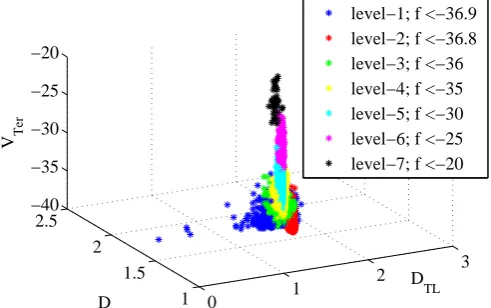
DIL, and trans-level DT L distance graph proposed in [1]. Minima are grouped, according to the value of their objective function, in levels, and for each levelDILis computed as the average value of the relative distance of each local minimum with respect to all other local minima within the same level, while DT L is the average value of the relative distance of each local minimum with respect to all other local minima in the lower level. TheDT Lfor the lowest level is computed as the average distance with respect to the best-known solution. The valuesDIL andDT L give an immediate representation of the diversity of the local minima and the probability of transition from one level to the lower one. Distances are computed by considering all variables normalized in [0,1]. The reader can find more details on the procedure in [1].

First two cases were chosen to demonstrate how the proposed code works on single funnel multimodal functions, which are challenging but usually solved by other codes in literature, but the vast majority of tests were performed on the third test case which is much harder and there were not optimal solutions available yet.

1) Tersoff Potential Function Minimization Problem: It is case 5 in the report [6]. The problem considers 10 silicon atoms, whose relative positions should be optimized to minimize the Tersoff potential, VT er,governing the inter-atomic interaction. The dimensionality of the problem is nD = 30, and bounds are: LB=[ 0, 0, 0, 4, 4, 4, -4.25, --4.25, --4.25, -4.5, -4.5, -4.5, -4.75, -4.75, -4.75, -5, 5, 5, 5.25, 5.25, 5.25, 5.5, 5.5, 5.5, 5.75, 5.75, -5.75, -6, -6, -6]; U B=[4, 4, π, 4, 4, 4, 4.25, 4.25, 4.25, 4.5, 4.5, 4.5, 4.75, 4.75, 4.75, 5, 5, 5, 5.25, 5.25, 5.25, 5.5, 5.5, 5.5, 5.75, 5.75, 5.75, 6, 6, 6]. The best solution found, with f = −36.929, is xopt=[ 1.5169, 0.048489, 0.85633, 0.38885, 1.0413, 0.032398, 0.30653, 2.1271, -0.46709, 1.9542, 2.6998, -0.87986, -0.5422, 0.13309, 2.0235, 0.67688, -1.8953, 1.904, 0.27924, 3.2425, -2.4656, 2.4006, 2.492, -3.1928, 0.91344, 0.98226, -2.1435, -1.6823, -1.9195, 1.7419].

As can be seen in Fig. 1, the search space is characterized by a single, multimodal funnel with a flat and broad low

0 1

2 3

1 1.5 2 2.5 −40 −35 −30 −25 −20

D

TL

D

IL

V Ter

level−1; f <−36.9 level−2; f <−36.8 level−3; f <−36 level−4; f <−35 level−5; f <−30 level−6; f <−25 level−7; f <−20

Fig. 1. Relative distances of the local minima for the Tersoff Potential case

0 0.5 1 1.5 2

2.5 1

1.5 2 0.5

1 1.5

D

TL

D

IL

AC

max

level−1; f <0.51 level−2; f <0.6 level−3; f <0.7 level−4; f <0.8 level−5; f <0.9 level−6; f <1 level−7; f <1.1 level−8; f <1.2

Fig. 2. Relative distances of the local minima for the Radar Polly phase Code Design case

region, f < −36.5, and two distinct basins for solutions with−36.9≤f ≤ −36.8 (red in Fig. 1), and solutions with f <−36.9(blue in Fig. 1). In what follows this problem is referred as Case 1.

2) Spread Spectrum Radar Polyphase Code Design: This test case is the number 7 in the CEC2011 report [6]. It is related to the polyphase pulse compression code synthesis, and is formulated as amin−maxoptimization problem, with nD = 20 design parameter. The objective is to minimize the module of the biggest among the samples of the so-called auto-correlation function, ACmax, which is related to the complex envelope of the compressed radar pulse at the optimal receiver output, while the variables represent sym-metrized phase differences [17] All variables are bounded

∈ [0,2π], and the best solution found, with f = 0.5, is xopt=[ 2.5725, 2.6228, 5.5686, 0.73972, 1.0953, 0.83449, 5.5796, 1.2897, 1.4654, 4.4623, 2.9833, 2.7519, 3.6232, 4.6328, 4.6773, 4.0213, 4.7433, 4.5053, 4.0768, 3.8608].

A. Messenger mission

The third test case is the optimization of a multigrav-ity assist trajectory with deep space manoeuvres (MGA-DSM)[13]: the multi-gravity assist transfer to Mercury, sim-ilar to the Messenger mission. The dimensionality of the problem isnD= 26and bounds and current known optimal solution are reported into Tab. I. In the table the solution vector is organized as in the ESA-ACT formulation [14]. As in the ESA-ACT formulation, the total∆V of the spacecraft is minimized. Note that the optimal solution shown in Tab. I has not been published elsewhere before.

TABLE I

BOUNDS AND OPTIMAL SOLUTION FORMESSENGER MISSION CASE -THE SOLUTION VECTOR IS REARRANGED AS IN THEESA-ACT

FORMULATION

LB U B Optimal

1900 2300 2038.03929616519 2.5 4.05 4.049996292063

0 1 0.556671418496 0 1 0.634280071715 100 500 451.600564550433 100 500 224.694751687357 100 500 221.839034379715 100 500 263.91480200672 100 500 359.354749401042 100 600 444.599274004631 0.01 0.99 0.607007547348 0.01 0.99 0.272048501594 0.01 0.99 0.692428663742 0.01 0.99 0.638908117493 0.01 0.99 0.829095716093 0.01 0.99 0.873723700599 1.1 6 1.774896822334 1.1 6 1.100004754835 1.05 6 1.050148253516 1.05 6 1.079891515997 1.05 6 1.40370492038

−π π 2.758595938641

−π π 1.575027216724

−π π 2.602608233794

−π π 2.272846047293

−π π 1.579719453208

0 0.5

1 1.5

2 2.5

0 1 2

D TL D

IL

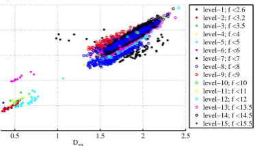
level−1; f <2.6 level−2; f <3.2 level−3; f <3.5 level−4; f <4 level−5; f <5 level−6; f <6 level−7; f <7 level−8; f <8 level−9; f <9 level−10; f <10 level−11; f <11 level−12; f <12 level−13; f <13.5 level−14; f <14.5 level−15; f <15.5

Fig. 3. Relative distances of the local minima for the Messenger mission case

The structure of the search space for the Messenger mission problem, as shown in Figs. (3) and (4), appears to be characterized by two main substructures. Solutions with

0.5 1 1.5 2 2.5 D

TL

level−1; f <2.6 level−2; f <3.2 level−3; f <3.5 level−4; f <4 level−5; f <5 level−6; f <6 level−7; f <7 level−8; f <8 level−9; f <9 level−10; f <10 level−11; f <11 level−12; f <12 level−13; f <13.5 level−14; f <14.5 level−15; f <15.5

Fig. 4. Relative distances of the local minima for the Messenger mission case - Plane view

∆V > 6km/s belong to a macro basin containing a very high number of local minima, characterized by big intra-level and trans-intra-level distances, and is a very large multi-modal funnel. On the other hand, optimal solutions, with ∆V < 6km/s, are located into a secondary basin, have smaller intra-level and trans-level distances, and the local structure is multi-funnel like.

IV. TESTRESULTS

In this Section the results of all test cases are presented and commented. The results on Cases 1 and 2 (see Sections III-.1 and III-.2) are described first, and then the space trajectory problem is used to further analyse the characteristics and critical aspects of the proposed algorithm. For all tests, the adopted DE strategy was DE/best/1/bin, tolconv = 0.2, δc= 0.1,CRC= 3and all reported statistics are computed on the results obtained from 100 independent runs.

A. Results on Cases 1 and 2

Few different settings of AIDEA were used to solve these problems, and the algorithm performed always very well, finding the global optima with high reliability within the limit of 1e5 function evaluations as required for the CEC 2011 competition. The embedded restart mechanism makes AIDEA perfectly suitable for solving problems with funnel like multimodal structures. In Tables (II) and (III) the results obtained by AIDEA on Case 1 and 2 are shown. AIDEA is set with npop = 20,iunmax = 10, δb = 0.1, where ±δb is added to current solution to create the local bubble for local restart (step 24 in Alg. (1)), and is compared to two of the best performing algorithms of the CEC 2011 competition, the Genetic Algorithm with Multi Parent Crossover (GA-MPC) [15] and the Weed Inspired Differential Evolution (WI-DE) [16].

TABLE II

RESULTS OFAIDEAONCASES1COMPARED TOWI-DEANDGA-MPC

Alg. M in M ean M ax Str.Dev.

AIDEA -36.9286 -36.8527 -35.5171 0.2442

W I−DE -36.8 -35.6 -34.2 0.904

TABLE III

RESULTS OFAIDEAONCASES2COMPARED TOWI-DEANDGA-MPC

Alg. M in M ean M ax Str.Dev.

AIDEA 0.5 0.5159 0.6384 0.0340

W I−DE 0.5 0.656 0.993 0.116

GA−M P C 0.5 0.7484 0.9334 0.1249

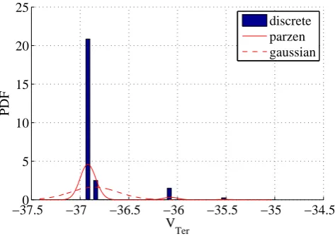
A better understanding of the performance obtained on these test cases can be achieved by looking at Figures (5) and 6), where the distribution of the best results obtained over the 100 runs are plotted for Case 1 and 2, respectively. As it is expected, when the algorithm can find the global optimum with high reliability, the distribution cannot be approximated by a Gaussian (dashed red curve in the figures) and converges to an exponential one. Moreover, due to the fact that the algorithm can stagnate only into certain basins, the distribution is in general multimodal and discontinuous, as it is evident in Fig. (5). In these cases the distribution can be better approximated by other means, such as the Parzen kernel approach used here (continuous red curve in the figures). It should be noted that the global minimum of case 1, fmin = −36.9286 is not generally reached by other algorithms [15], [16] which stagnate on the solution fmin=−36.84(second peak from left in Fig. (5).

−37.50 −37 −36.5 −36 −35.5 −35 −34.5

5 10 15 20 25

V

Ter

PDF

discrete parzen gaussian

Fig. 5. Distributions of best results obtained by AIDEA (npop = 40, iunmax= 20,δb= 0.2) on Case 1

B. Results on Messenger mission

In order to better evaluate the performance and critical aspects of the proposed algorithm on a more difficult and challenging problem, both AIDEA and IDEA were run on the Messenger mission test case with different settings. From the results of the 2011 competition it appeared evident that none of the algorithms achieved near optimal solutions, since none of them was able to jump into the secondary structure of the problem (see Figs. 3 and 4) within the1.5e5function evaluations limit [15], [16]. For this work 5e6 function evaluations were considered and, again, all reported statistics

0.4 0.45 0.5 0.55 0.6 0.65 0.7 0.75

0 50 100 150 200

AC

max

PDF

discrete parzen gaussian

Fig. 6. Distributions of best results obtained by AIDEA (npop = 40, iunmax= 20,δb= 0.2) on Case 2

were computed on the results obtained from 100 independent runs.

First a direct comparison between IDEA and AIDEA with equal values of common parameters was performed. Here the case with npop = 40, iunmax = 20, and δb = 0.2 is reported. Main results for AIDEA and six different instances of IDEA are summarized in Tab. (IV). As it can be expected, IDEA can have optimal performance, if DE is well tuned, as in the case (F, CR) = (0.5,0.9), but performance can get considerably worse, if F and CR are mis-tuned, as in the case (F, CR) = (0.9,0.5). On the other hand, performance of AIDEA for this test benchmark are always just below those obtained by the best tuned IDEA, also when different values of npop,iunmax, andδb are considered.

TABLE IV

COMPARISON BETWEENIDEA (npop= 40,iunmax= 20,δb= 0.2)

ANDAIDEAPERFORMANCE ONMESSENGER CASE OVER100RUNS AFTER5e6FUNCTION EVALUATIONS- THE FIRST COLUMN CONTAINS

THE VALUES OFFANDCRUSED FORIDEA

F, CR M in M ean M ax Str.Dev.

0.1,0.5 3.1792 5.9029 8.4344 0.9158

0.1,0.9 3.1774 6.1825 8.1495 0.9254

0.5,0.5 3.2385 6.2099 13.8993 1.6175

0.5,0.9 2.7784 5.1268 6.3625 1.1023

0.9,0.5 6.2466 10.8371 15.6773 3.2088

0.9,0.9 3.2829 6.1514 7.5227 0.6653

AIDEA 3.1270 5.3790 6.4898 0.9218

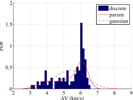
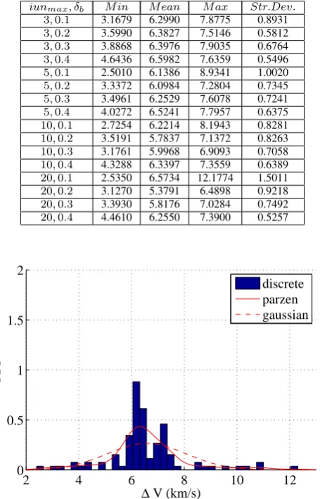
multimodal, with peaks revealing the attraction basins, and a kernel based approach could be better used to approximate the PDF. For the case in hand, histograms confirm that the performance of AIDEA are close to the best IDEA, and for both cases the solutions in the basins with ∆V < 6 are almost equally distributed.

2 3 4 5 6 7 8 9

0 0.5 1 1.5 2

∆V (km/s)

PDF

discrete parzen gaussian

Fig. 7. Distributions of best results obtained by AIDEA (npop = 40, iunmax= 20,δb= 0.2) on Messenger case

2 3 4 5 6 7 8 9

0 0.5 1 1.5 2

∆V (km/s)

PDF

discrete parzen gaussian

Fig. 8. Distributions of best results obtained by IDEA (npop = 40, iunmax= 20,δb= 0.2,F= 0.1,CR= 0.9) on Messenger case

The evolution of performance with the number of function evaluations for AIDEA and the best IDEA is given in Fig. (10). Data are shown from1.5e5function evaluations, which is the maximum value for the CEC 2011 competition, to5e6. In both cases, the performance obtained at1.5e5function evaluations are comparable with the best performance ob-tained by other algorithms during the competition [15], [16], as reported in Tab. V, but, differently from what happens to other algorithms, performance keep improving with the number of function evaluations, mainly due to the restart mechanism preventing stagnation.

2 3 4 5 6 7 8 9

0 0.5 1 1.5 2

∆ V (km/s)

PDF

discrete parzen gaussian

Fig. 9. Distributions of best results obtained by IDEA (npop = 40, iunmax= 20,δb= 0.2,F= 0.5,CR= 0.9) on Messenger case

0 0.5 1 1.5 2 2.5 3 3.5 4 4.5 5

x 106

0 5 10 15 20

Num. of Func. Eval.

Best Sol. (km/s)

AIDEA Min AIDEA Mean AIDEA Max IDEA Min IDEA Mean IDEA Max

Fig. 10. Evolution of best results obtained by AIDEA (npop = 40, iunmax= 20,δb= 0.2) and IDEA (F= 0.5,CR= 0.9) on Messenger case

In Figure 11 the performance of the Genetic Algorithm with Multi-Parent Crossover (GA-MPC) [15] with population size= 200are plotted as function of the function evaluations up to1e6and it can be seen that the algorithm stagnate after 2e5evaluations.

TABLE V

COMPARISON AMONGAIDEA (npop= 40) WI-DEANDGA-MPCON

MESSENGER CASE FOR1.5e5FUNCTION EVALUATIONS

Alg. M in M ean M ax Str.Dev.

AIDEA 4.3008 11.16029 15.7070 2.9550

W I−DE 6.78 11.5 13.2 2.44

GA−M P C 7.0956 1.2818 1.6925 3.2413

0 2 4 6 8 10

x 105

0 10 20 30 40 50

Function evaluations

∆

V (km/s)

Mean Min Max

Fig. 11. Evolution of best results obtained by GA-MPC (npop= 200) on Messenger case

the effect of a too small local bubble, such as in the case (iunmax, δb) = (20,0.1). As can be seen in Fig. (12), the algorithm with this setting can get stuck into zones with high values (∆V >7km/s) of the objective function and is not able to perform the transition to lower levels, or, overall, to the secondary structure containing the global optimum, within the allowed number of function evaluations.

The combinationiunmax, δbhas almost the same influence on the performance also if different population sizes are considered, as can be seen in Tables VII and VIII where the same statistics are reported for tests withnpop= 20and npop = 10, respectively. The comparison of the statistics in the three Tables also demonstrates that the AIDEA is robust against different values of the populations size. It is worth noting that the population size of the embedded DE should be much smaller than the size of a standard DE, to allow a faster convergence and multiple following restarts.

The analysis of the results for this complex test case con-firm the validity of the inflationary approach, which is made more robust by the technique for the on-line adaptation of DE control parameters. On the other hand, tests also make clear that to further enhance the algorithm other critical parameters should be automatically set during the optimization process. The population size is for sure one of them, but a correct combination of number of local restarts and dimension of local bubble is even more critical for a system much relying on restart both to exploit (local restart) and explore (global restart) the search space.

TABLE VI

PARAMETRIC ANALYSIS FORAIDEAPERFORMANCE(npop= 40)ON

MESSENGER CASE- THE FIRST COLUMN CONTAINS THE USED VALUES OFiunmaxANDδb

iunmax, δb M in M ean M ax Str.Dev.

3,0.1 3.1679 6.2990 7.8775 0.8931

3,0.2 3.5990 6.3827 7.5146 0.5812

3,0.3 3.8868 6.3976 7.9035 0.6764

3,0.4 4.6436 6.5982 7.6359 0.5496

5,0.1 2.5010 6.1386 8.9341 1.0020

5,0.2 3.3372 6.0984 7.2804 0.7345

5,0.3 3.4961 6.2529 7.6078 0.7241

5,0.4 4.0272 6.5241 7.7957 0.6375

10,0.1 2.7254 6.2214 8.1943 0.8281

10,0.2 3.5191 5.7837 7.1372 0.8263

10,0.3 3.1761 5.9968 6.9093 0.7058

10,0.4 4.3288 6.3397 7.3559 0.6389

20,0.1 2.5350 6.5734 12.1774 1.5011

20,0.2 3.1270 5.3791 6.4898 0.9218

20,0.3 3.3930 5.8176 7.0284 0.7492

20,0.4 4.4610 6.2550 7.3900 0.5257

2 4 6 8 10 12

0 0.5 1 1.5 2

∆ V (km/s)

PDF

discrete parzen gaussian

Fig. 12. Distributions of best results obtained by AIDEA (npop = 40, iunmax= 20,δb= 0.1) on Messenger case

Another feature that should be embedded into future versions of the code is the on-line learning of the currently best DE strategy. Preliminary tests show that if the algorithm is exploring a near optimal region, strategyDE/rand/1/bin could be beneficial to escape local structures and converge to the optimal point. But, again, if strategyDE/rand/1/binis used when the AIDEA is exploring the big basin with high ∆V’s, many function evaluations are spent to converge into the non optimal basin.

V. CONCLUSIONS

TABLE VII

PARAMETRIC ANALYSIS FORAIDEAPERFORMANCE(npop= 20)ON

MESSENGER CASE- THE FIRST COLUMN CONTAINS THE USED VALUES OFiunmaxANDδb

iunmax, δb M in M ean M ax Str.Dev.

3,0.1 3.0618 6.2296 7.4400 0.7907

3,0.2 4.4258 6.4749 7.4035 0.5033

3,0.3 3.5811 6.3763 8.1853 0.6909

3,0.4 4.9969 6.7633 9.2208 0.6720

5,0.1 2.8336 6.2347 7.5139 0.8904

5,0.2 3.6415 6.2126 7.6438 0.7790

5,0.3 3.6754 6.4785 7.6099 0.5969

5,0.4 4.9621 6.6339 7.8255 0.5207

10,0.1 3.1494 6.2401 10.8552 1.1323

10,0.2 3.0285 6.0034 7.0366 0.8189

10,0.3 3.8668 6.2699 7.4899 0.5861

10,0.4 5.0080 6.5426 7.7897 0.4925

20,0.1 3.0627 6.2828 10.9439 1.4119

20,0.2 3.3786 5.8209 7.1450 0.6697

20,0.3 3.5840 5.9849 7.3529 0.7348

20,0.4 4.8674 6.2601 7.3455 0.4910

TABLE VIII

PARAMETRIC ANALYSIS FORAIDEAPERFORMANCE(npop= 10)ON

MESSENGER CASE- THE FIRST COLUMN CONTAINS THE USED VALUES OFiunmaxANDδb

iunmax, δb M in M ean M ax Str.Dev.

3,0.1 3.0607 6.4858 8.6385 0.8691

3,0.2 3.9232 6.4844 9.2189 0.8424

3,0.3 3.3621 6.7159 9.5182 0.7731

3,0.4 5.4851 6.9356 8.1869 0.5747

5,0.1 4.0149 6.3407 8.7837 0.8755

5,0.2 3.1930 6.3255 8.3996 0.7947

5,0.3 4.0601 6.6772 8.2935 0.7209

5,0.4 4.1606 6.7243 8.2624 0.7036

10,0.1 2.6851 6.0550 7.8807 1.0203

10,0.2 3.4241 6.0912 7.4743 0.7217

10,0.3 4.3824 6.4754 8.1999 0.6169

10,0.4 4.7132 6.7901 7.8223 0.5189

20,0.1 2.5044 6.1944 9.6058 1.4632

20,0.2 3.1834 5.8817 7.0045 0.7866

20,0.3 3.9548 6.1134 7.4883 0.6643

20,0.4 3.7572 6.4462 8.0238 0.6797

on the CEC2011 competition.

The sensitivity analysis on the most difficult problem, the Messenger mission, has shown that the on-line adaptation of the parameters regulating the local restart procedure is a cru-cial aspect. Furthermore, a clever adaptation of DE strategy could better balance convergence and exploration especially in cases, like the Messenger problem, where the structure of the landscape changes radically when approaching lower values of the cost function.

REFERENCES

[1] M. Vasile, E. Minisci, M. Locatelli, “An Inflationary Differential Evolution Algorithm for Space Trajectory Optimization,”IEEE Trans. on Evolutionary Computation, vol. 15, no. 2, pp. 267-281, 2011. [2] K.V. Price, R.M. Storn, J.A. Lampinen, “Differential Evolution. A

Practical Approach to Global Optimization,”Natural Computing Se-ries,Springer, 2005.

[3] D.J. Wales, J.P.K. Doye, “Global optimization by basin-hopping and the lowest energy structures of Lennard-Jones clusters containing up to 110 atoms,”J. Phys. Chem. A, vol. 101, pp. 51115116, 1997. [4] B.Addis, M. Locatelli, F.Schoen, “Local optima smoothing for global

optimization,”Optimization Methods and Software, vol. 20, pp. 417-437, 2005.

[5] S. Das, P.N. Suganthan, “Differential Evolution: A Survey of the State-of-the-Art,”IEEE Trans. on Evolutionary Computation, vol. 15, no. 1, pp. 4-31, 2011.

[6] S. Das, P.N. Suganthan, “Problem Definitions and Evaluation Criteria for CEC 2011 Competition on Testing Evolutionary Algorithms on Real World Optimization Problems,”Technical Report, 2010. [7] J. Liu and J. Lampinen, “A fuzzy adaptive differential evolution

algorithm,”Soft Comput. A Fusion Founda. Methodol. Applicat., vol. 9, no. 6, pp. 448462, 2005.

[8] A.K. Qin, V.L. Huang, P. N. Suganthan, “Differential evolution al-gorithm with strategy adaptation for global numerical optimization,” IEEE Trans. Evol. Comput., vol. 13, no. 2, pp. 398417, 2009. [9] M. M. Ali and A. Trn, “Population set based global optimization

algorithms: Some modifications and numerical studies,”Comput. Oper. Res., vol. 31, no. 10, pp. 17031725, 2004.

[10] J. Brest, S. Greiner, B. Boskovic, M. Mernik, V. Zumer, “Self-adapting control parameters in differential evolution: A comparative study on numerical benchmark problems,”

[11] R. Storn, “Differential evolution research: Trends and open questions,”

InAdvances in Differential Evolution, U.K. Chakraborty, Ed. Berlin,

Germany: Springer, pp. 132, 2008.

[12] K. Fukunaga, “Introduction to Statistical Pattern Recognition,” Aca-demic Press, New York, 1972.

[13] M. Vasile M., P. De Pascale, “Preliminary Design of Multiple Gravity-Assist Trajectories,”J. of Spacecraft and Rockets, vol. 43, no. 4, 2006.

[14] http://www.esa.int/gsp/ACT/inf/op/globopt/MessengerFull.html

[15] S.M. Elsayed, R.A. Sarker, D.L. Essam, “GA with a New Multi-Parent Crossover for Solving IEEE-CEC2011 Competition Problems,” In: IEEE Congress on Evolutionary Computation, pp. 1034-1040, 2011. [16] U. Halder, S. Das, D. Maity, A. Abraham, P. Dasgupta, “Self Adaptive

Cluster Based and Weed Inspired Differential Evolution Algorithm For Real World Optimization”, In:IEEE Congress on Evolutionary Computation, pp. 750-756, 2011.