Cost-sensitive adaboost algorithm for ordinal regression based on extreme learning machine

A Cost-Sensitive AdaBoost algorithm for Ordinal

Regression based on Extreme Learning Machine

Annalisa Riccardi, Francisco Fern´andez-Navarro,

Member IEEE

and Sante Carloni

Abstract—In this paper, the well-known Stagewise Additive

1

Modeling using a Multi-class Exponential (SAMME) boosting

2

algorithm is extended to address problems where there exists a

3

natural order in the targets using a cost-sensitive approach. The

4

proposed ensemble model uses as a base classifier an Extreme

5

Learning Machine (ELM) model, (with the Gaussian kernel and

6

the additional regularization parameter). The closed form of the

7

derived Weighted Least Squares Problem (WLSP) is provided

8

and it is employed to estimate analytically the parameters

9

connecting the hidden layer to the output layer at each iteration

10

of the boosting algorithm. Compared to the state-of-the-art

11

boosting algorithms, in particular those using ELM as base

12

classifier, the suggested technique doesn’t require the generation

13

of a new training dataset at each iteration. The adoption of

14

the weighted least squares formulation of the problem has been

15

presented as an unbiased and alternative approach to the already

16

existing ELM boosting techniques. Moreover, the addition of a

17

cost model for weighting the patterns, according to the order

18

of the targets, extends further the classifier to tackle ordinal

19

regression problems. The proposed method has been validated

20

by an experimental study with comparison to already existing

21

ensemble methods and ELM techniques for ordinal regression,

22

showing competitive results.

23

Index Terms—Ordinal Regression, Boosting, SAMME

algo-24

rithm, Extreme Learning Machine, Neural Networks

25

I. INTRODUCTION 26

Ordinal regression resides between multi-classification and 27

standard regression in the area of supervised learning. In an 28

ordinal regression problem, the patterns are labeled with a set 29

of discrete ranks [1], [2], [3], [4]. It is commonly formulated 30

as a multi-class problem with ordinal constraints [5], [6]. The 31

goal of learning in ordinal regression is to find a model based 32

on training set which can predict the rank of the patterns in 33

the test set. Several approaches for ordinal regression were 34

proposed in recent years from a machine learning perspective. 35

Vast majority of the algorithms are based on the idea of 36

transforming the ordinal scales into numeric values, and then 37

solving the problem as a standard regression problem [5], [7], 38

[8], [9], [10]. This kind of algorithms are called threshold 39

models. Two examples of threshold algorithms are the support 40

vector based formulations [11], [12] and the Gaussian Process 41

for Ordinal Regression (GPOR) [13] method. 42

In the field of Extreme Learning Machines (ELMs), Deng 43

et al. [14] proposed a modification in the encoding scheme 44

to adapt the standard ELM algorithm to the ordinal scenario. 45

They considered three methodologies with its corresponding 46

All the authors are with the Advanced Concepts Team, Euro-pean Space Research and Technology Centre (ESTEC), European Space Agency (ESA), 2201 AZ Noordwijk, Netherlands, e-mail: [email protected], [email protected],[email protected] and [email protected]

encoding schemes: the single multi-output classifier approach, 47

the multiple binary-classifications with one-against-all decom-48

position method and the one-against-one method. After that, 49

the models parameters are trained using the corresponding 50

encoding framework. From another perspective, Becerra et al. 51

[15] proposed an evolutionary approach based on the Evolu-52

tionary ELM (E-ELM) [16] to address the ordinal regression 53

problem. The authors relied on the assumption that the ordinal 54

structure of the set of class labels is also reflected in the 55

topology of the instance space. Under this idea, Becerra et 56

al. [15] proposed an evolutionary algorithm in two stages. 57

The first stage makes a projection of the ordinal structure of 58

the feature space. Next, an evolutionary algorithm tunes the 59

first projection working with the misclassified patterns near 60

the border of their right class. 61

On the other hand, ensembles are a promising machine 62

learning research field, where several models are combined 63

to generate a final output [17], [18], [19]. Two factors must 64

be considered in order to enhance the generalization per-65

formance of a neural network ensemble. One is diversity 66

and the other one is the performance of the models that 67

comprise the ensemble. A trade-off study between the optimal 68

measures of diversity and performance is available in [18]. The 69

approaches for designing neural network ensembles can be 70

divided in two groups: the first one iterates between different 71

architectures and parameters settings while the second one 72

gets diverse models by training them on different training 73

sets. Some approaches on this idea are bagging, boosting or 74

cross-validation [20], [21], [22]. Both groups of methodologies 75

directly generate a group of neural networks which are error 76

uncorrelated. 77

For ordinal regression problems, there are some ensemble-78

related approaches. The main idea of these approaches is 79

to transform the classification problem into a nested binary 80

classification one, and then combine the resulting classifier 81

predictions to obtain the final ensemble model. For example, 82

Frank and Hall [23] proposed a general algorithm that enables 83

binary classifiers to make use of order information in the 84

targets, using as base binary classifier a tree model. Waegeman 85

and Boullart [24] proposed an enhanced method based on 86

an ensemble of Support Vector Machines (SVMs). In their 87

proposal, each binary classifier is trained with specific weights 88

for each pattern of the training set. 89

Recently, two neural network threshold ensemble models for 90

ordinal regression have been proposed in [10], [25]. For the 91

first ensemble method, the thresholds are fixed a priori and 92

are not modified during training. The second one considers 93

the thresholds of each member of the ensemble as free 94

process. This is achieved through a reformulation of the 1

tunable thresholds to avoid the definition of constraints in the 2

ordinal regression problem. During training diversity, existing 3

in the different projections generated by each member, is 4

taken into account for the parameter updating according to the 5

Negative Correlation Learning (NCL) framework [26], [27]. 6

In the NCL framework, an ensemble of M neural networks 7

are trained in parallel using gradient descent techniques. The 8

error function for each neural network, in addition to the usual 9

squared error term, contains a penalty term proportional to the 10

correlation of the network projections with those of all the 11

other networks. The ordinal thresholds ensemble models of 12

[10], [25] were validated using an economic dataset and real 13

benchmark ordinal datasets 14

From another point of view, Perez-Ortiz et al. [28] proposed 15

a projection-based ensemble model where every single model 16

is trained in order to distinguish between one given class (j) 17

and all the remaining ones, while grouping them in those 18

classes with a rank lower than j, and those with a rank 19

higher than j. Actually, the proposal could be considered as 20

a reformulation of the well-known one-versus-all scheme. In 21

the study, the base algorithm for the ensemble could be any 22

threshold (or even probabilistic) model. 23

From a boosting perspective, two algorithms (ORBoost 24

and AdaBoost.OR) [29], [30] were proposed for the ordinal 25

scenario. ORBoost is a thresholded ensemble model for or-26

dinal regression which consists of a weighted ensemble of 27

confidence functions and an ordered vector of thresholds. In 28

[29], the authors also derived novel large margin bounds of 29

common error functions, such as the classification error and 30

the absolute error. Apart from this boosting approach based 31

on binary confidence functions, the same authors proposed 32

an extension of the well-known AdaBoost using the reverse 33

technique to directly improve the performance of existing cost-34

sensitive ordinal ranking algorithms, AdaBoost.OR [30]. 35

In this paper, the Stagewise Additive Modeling using a 36

Multi-class Exponential (SAMME) boosting algorithm [31] is 37

extended to address ordinal problems. The SAMME model 38

is an alternative approach to the multi class boosting algo-39

rithm called AdaBoost.MH [32]. The AdaBoost.MH algorithm 40

addresses the multi class problem performing J one-against-41

all classifications, where J is the number of classes, while 42

SAMME performs directly theJ class classification problem. 43

SAMME only needs weak classifiers better than random guess 44

(e.g. correct probability larger than1_{/J), rather than better than}

45

1_{/2 as the two-class AdaBoost requires.}

46

The proposed ensemble model uses as a base classifier an 47

Extreme Learning Machine (ELM) [33] model. Concretely, in 48

this work the Gaussian kernel version of the ELM with the 49

regularization parameter has been considered. The approach 50

integrates the advantages of variable weighting and the speed 51

of ELM. In each iteration of the SAMME algorithm, non-52

negative weights are assigned to different time steps of the 53

boosting process, reflecting the importance of each pattern in 54

each interval. The parameters corresponding to the linear part 55

of the model are analytically determined in each iteration ac-56

cording to the closed form of the Weighted Least Squares Error 57

(WLSE). Traditionally, the state-of-the-art boosting algorithms 58

using ELM as base classifier generate a new training subset 59

at each iteration. This task is unnecessary if the closed form 60

of the weighted least squares problems is adopted. 61

Summarizing, the main contributions of this paper are: 62

• The adaptation of the multi-class SAMME algorithm 63

to the ordinal scenario considering a cost-sensitive ap-64

proach. 65

• The use of a ELM model with Gaussian kernel and 66

the regularization parameter as base classifier (for its 67

competitive trade-off between efficiency and accuracy). 68

• The WLS closed-form solution of the error function 69

was considered to estimate the linear parameters of the 70

individuals in the final ensemble model. This avoids to 71

generate M different sub-datasets, where M is the size 72

of the ensemble, differently from what has been done 73

traditionally in the ELM community [34], [35], [36]. 74

The remainder of the paper is organised as follows: a brief 75

analysis of the SAMME algorithm for multi-class classifi-76

cation is given in Section II. Section III describes the cost-77

sensitive ensemble model proposed and Section IV draws the 78

way to estimate analytically the parameters of the ELM classi-79

fier based on the WLSE. Section V presents the experimental 80

framework while the results are discussed in Section VI. 81

Finally, Section VII summarises the achievements and outlines 82

some future developments of the proposed methodology. 83

II. MULTI-CLASSADABOOST 84

In this paper, the so-called Stagewise Additive Modeling 85

using a Multi-class Exponential loss function (SAMME) [31], 86

multi-class version of the AdaBoost method, is adopted. 87

SAMME directly handles the J-class problem by building 88

a single J-class classifier, instead of J binary ones. Zhu et 89

al. [31] proves that the solution of SAMME is consistent 90

with the Bayes classification rule, so it is optimal in mini-91

mizing the misclassification error. Given a training set D = 92

{X,C}={xn, cn}Nn=1, wherexn = (x1n, x2n, . . . , xKn)∈RK 93

and cn ∈ {1. . . J} ⊂ N is the n-th input pattern and its

94

corresponding target, the goal is to find a regression function 95

f : _RK _→

RJ, i.e., f(x) = (f1(x), . . . , fJ(x)) such that 96

minimizes the following error function: 97

min

f(x)

N

X

n=1

L(yn,f(xn)) (1)

s.t f1(xn) +. . .+fJ(xn) = 0, ∀n= 1, . . . , N

where 98

L(yn,f(xn)) = exp −1_/J(y1

nf1(xn) +. . .+y J

nfJ(xn))

= exp −1_/JyT

nf(xn)

,

is the exponential loss function for then-th pattern and 99

yn = (y1n, . . . , y J

n), (2)

is theJ-dimensional vector, encoding of the targetcn, defined 100

for allj= 1, . . . J as 101

ynj =

1 ifcn=j,

− 1

J−1 ifcn6=j.

SAMME Algorithm:

Require: Training dataset (D)

Require: Size of the ensemble (M)

Ensure: Ensemble model

1: w(1)n ←1/N,∀n= 1, . . . , N {Initialization of the patterns weights}

2: Initialization of the parameters of the ensemble model 3: form= 1, . . . , M do

4: Fit a classifier to the training set using weightswn(m)

5: e(m)_←PN n=1w

(m)

n I(o(m)(xn)6=cn)/PN_n=1w(nm) {Computation of the error of the weighted ELM model}

6: α(m)_←log1−e(m)

e(m) + log(J−1) 7: w(nm+1)←w

(m)

n exp(α(m)I(o(m)(xn)6=cn)),∀n= 1, . . . , N {Updating the weights}

8: w(nm+1)←w

(m+1)

n /PNn=1w

(m+1)

n ,∀n= 1, . . . , N {Normalization of the weights}

9: end for

10: Output:C(x) = arg max

j

PM m=1α

(m)

I(o(m)(x) =j)

11: return Ensemble model

Fig. 1: SAMME training algorithm framework

The symmetric constraint f1(xn) + . . . +fJ(xn) = 0 is 1

included to guarantee the unicity of the solution f, since 2

adding a constant to all fj(xn) will give the same loss as 3

PJ

j=1y

j

n = 0 for every n ∈ {1, ..., N}. As proved in [31] 4

the formulation of Problem 1 is consistent with the Bayes 5

classification rule. 6

Fig. 1 describes the algorithmic flow of the SAMME 7

algorithm, where w(nm) is the weight of the n-th pattern, at 8

the m-th iteration of the ensemble model, and o(m)_(x

n) is 9

the index of the maximum component of the corresponding 10

predicted values 11

o(m)(xn) = arg maxf(m)(xn), (4)

withf(m)_{(xn)them-th classifier,I(·)is the indicator function}

12

(I(x) = 0 if x is false, 1 otherwise) and C(x) is the class 13

predicted by the ensemble model for the test pattern x. 14

From Fig. 1, it is possible to recognise which is the main 15

difference between SAMME and two-class AdaBoost. This 16

difference resides in Step 6 of Fig. 1. A furtherlog(J−1)term 17

is added to guarantee the positiveness of the exponent α(m)

18

(and hence the increasing of the corresponding weight for the 19

misclassified pattern) when the weighted errore(m)_<(J−1)_/J,

20

at each iteration m of the ensemble model. In the case of 21

J = 2, the SAMME algorithm is equivalent to the original 22

two-class AdaBoost because log(J−1) = 0. 23

III. COSTSENSITIVEADABOOST FORORDINAL 24

REGRESSION 25

In ordinal regression problems exists an order relation 26

between labels, such as C1 ≺ C2 ≺. . .CJ, where ≺denotes 27

the given order between different ranks. To be compliant 28

with the previous notation, a bijection between the labels 29

set{Cj}Jj=1 and integer values{1, . . . , J}is established, that

30

maintains the order, such asCj ↔j. 31

Based on the approach of [37], designed to tackle combi-32

natorial and imbalanced datasets with a cost-sensitive boost-33

ing classifier, a cost model that encodes the penalty of the 34

misclassified patterns for ordinal regression problems is intro-35

duced in the ensemble model here proposed. The cost matrix 36

K ∈RJ×RJ used to encode the penalty of the misclassified

37

patterns is the Absolute cost matrix reported in Table I, for 38

the particular case of a 5-class classification problem, where 39

the element at position(i, j)represents the cost of classifying 40

a pattern of class ias pattern of classj 1. 41

TABLE I: Example of different cost matrices.

Zero-one Absolute cost Quadratic cost 

   

0 1 1 1 1

1 0 1 1 1

1 1 0 1 1

1 1 1 0 1

1 1 1 1 0



   



   

0 1 2 3 4

1 0 1 2 3

2 1 0 1 2

3 2 1 0 1

4 3 2 1 0



   



   

0 1 4 9 16

1 0 1 4 9

4 1 0 1 4

9 4 1 0 1

16 9 4 1 0



   

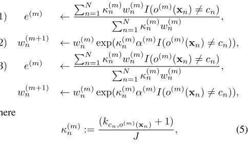
Three cost-sensitive variants of the SAMME algorithm 42

are provided. To guarantee the equivalence to the stagewise 43

additive modeling three different loss functions are used 44

1) L1(yn,f(xn)) =κnexp(−1/JyT_nf(xn)), 45

2) L2(yn,f(xn)) = exp(−κn/JyT_nf(xn)), 46

3) L3(yn,f(xn)) =κnexp(−κn/JyT_nf(xn)), 47

whereκnrepresents the cost of misclassifying then-th pattern. 48

Each formulation affect the update rule of the error estimation 49

and/or of the pattern weights at the m-th iteration of the 50

ensemble model (where the weights used in the following 51

iteration are determined). In particular 52

1) e(m) _←

PN

n=1κ (m)

n w

(m)

n I(o(m)(xn)6=cn)

PN

n=1κ (m)

n w(nm)

,

2) w(nm+1) ←w(nm)exp(κ

(m)

n α

(m)_I(o(m)_(xn)6=cn)),

3) e(m) _←

PN

n=1κ (m)

n w

(m)

n I(o(m)(xn)6=cn)

PN

n=1κ (m)

n w

(m)

n

,

w(nm+1) ←w(nm)exp(κ

(m)

n α

(m)

I(o(m)(xn)6=cn)),

where 53

κ(_nm):= (kcn,o(m)(xn)+ 1)

J , (5)

1_{Please note that all the cost matrices in Table I are symmetric. It is}

with k_cn,o(m)_(xn) the (cn, o(m)(xn))-element of the cost ma-1

trix, hence the cost of misclassifying patternxnof classcn as 2

pattern of the class o(m)_(x

n); J is introduced for robustness 3

as normalization factor and 1 is added to avoid zeroing the 4

equation. If compared with [37], where only one cost value is 5

assigned to the misclassification of each pattern, the proposed 6

model includes a cost schema,κ(nm), whose values depend on 7

the prediction of the m-th model. 8

For the details of the proof of equivalence with the stagewise 9

additive modeling please refer to [31]. 10

IV. WEIGHTEDLEASTSQUARESESTIMATION FOR 11

EXTREMELEARNINGMACHINE 12

Extreme Learning Machine (ELM) is an efficient algorithm 13

that determines the output weights of a Single Layer Feedfor-14

ward Neural Network (SLFNN) using an analytical solution 15

instead of the standard gradient descent algorithm [39]. ELM 16

have been used to solve classification and regression problems 17

in several domains ranging from computer vision [40], credit 18

risk evaluation [41] or bioinformatics [42]. 19

Traditionally, for a SLFNN, all the parameters for the 20

different layers need to be tuned and there is a dependency 21

among the different layers. The gradient descent algorithm is 22

slow and is prone to converge to local minima. Furthermore, to 23

achieve good generalization performance several iterative steps 24

are necessary [33], [43], [44]. The ELM scheme proposed by 25

Huang et. al. [43] overcomes these problems by randomly as-26

signing weights to the input layers and analytically computing 27

the weights for the output layer using a simple generalized 28

inverse operation. The ELM framework has shown comparable 29

classification performance, and faster run times in comparison 30

to support vector machines [45], [46]. 31

Let’s note as vs = (vs1, vs2, . . . , vsK) the weight vector 32

connecting the input nodes to the s-th basis function, for 33

s= 1,2, . . . , S and withβj= (β₁j, . . . , β_Sj)the weight vector 34

connecting the basis functions to the j-th output node for 35

j = 1, . . . , J. 36

During the training process, ELM determines the parameters 37

βj, for all j values, by minimizing the Least Squared Error 38

(LSE) function: 39

LSE = N

X

n=1

J

X

j=1

(fj(xn)−y_nj)2, (6)

wherefj(xn)is the estimated output corresponding to then-th 40

input pattern and thej-th class. It is defined as: 41

fj(xn) = S

X

s=1

βj_sφ(xn;vs), n∈ {1, . . . , N}, (7)

whereφ(xn;vs)is the activation function. According to [47] 42

the concurrent minimization of the training error and the 43

norm of the weight parameters, allows better generalization 44

performance for the network. Hence the minimization problem 45

has the following form 46

min

β∈RS×RJ

kHβ−Yk2_{, kβk}

(8)

wherek·kis the L2 norm,His the hidden layer output matrix of the SLFN:

H= (h1,h2, . . . ,hS) =

=





φ1(x1;v1) . . . φS(x1;vS)

. . . . φ1(xN;v1) . . . φS(xN;vS)



∈R

N

×RS (9)

Y= (y1,y2, . . . ,yN)T ∈RN ×RJ, (10)

and 47

β= (β1,β2, . . . ,βJ)∈RS×RJ. (11)

The ELM algorithm starts choosing the activation function 48

φ(x,v) and the number of basis functions S. Generally, the 49

sigmoidal function is the one selected in the ELM framework 50

although other types of basis functions could be also consid-51

ered [48], [49]. In the first step, arbitrary weights are assigned 52

to the input weight vectors vs. The problem of minimizing 53

the training error reduces to solve the linear system 54

Hβ=Y. (12)

Therefore the output weights β are approximated by the 55

Moore-Penrose generalized inverse [43], [44], to guarantee 56

better generalization performance [50], 57

ˆ

β=H†Y, (13)

where

H†=

(

HT I

C+HH T−1

for N < S, I

C +H T_H−1

HT _otherwise, (14)

and C ∈ R is a user-specified parameter that promotes

58

generalization performance. 59

Traditionally Boosting algorithms proceed by continuously 60

minimizing the Weighted Least Square Error (WLSE) between 61

the estimated outputs and its true target. In the field of ELM, 62

several adaptations of the original AdaBoost algorithm have 63

been proposed for regression and classification problems [34], 64

[35], [36]. These approaches use the AdaBoost algorithm to 65

generate M training subsets from the training set, and then 66

train one ELM regressor/classifier for each of training subsets, 67

henceM regressors/classifiers are finally obtained. 68

In this work, the weights distribution is employed to directly 69

estimate the β parameters instead of using it to generateM

70

different sub-datasets. The generation of theseM sub-datasets 71

is unnecessary if the WLSE is adopted. Therefore, the goal is 72

to find the parameter matrix β which minimizes the WLSE 73

for allnpatterns in the training set with weightwn, i.e.: 74

WLSE = N

X

n=1

J

X

j=1

wn(fj(xn)−y_nj)2. (15)

As before, to improve the generalization performance, the 75

norm of the weights need to be minimized concurrently. 76

Therefore the problem can be formulated as 77

min

β∈RS×RJ

(Hβ−Y)TW(Hβ−Y), kβk

AdaBoost(ELM) Algorithm:

Require: Training dataset (D)

Require: Size of the ensemble (M)

Require: Regularization Parameter (C)

Require: Width Gaussian Kernel (k)

Ensure: ELM Ensemble model

1: w(1)n ←1/N,∀n= 1, . . . , N {Initialization of the patterns weights}

2: Estimation ofΩELM

3: Initialization of the parameters of the ensemble model 4: form= 1, . . . , M do

5: f(m)(x) :=K(x)T_CI +W(m)ΩELM

−1

W(m)Y{Computation of the kernelized output function}

6: e(m)←PN n=1w

(m)

n I(o(m)(xn)6=cn)/PNn=1w (m)

n {Computation of the error of the weighted ELM model}

7: α(m)←log1−e(m)

e(m) + log(J−1)

8: w(nm+1)←wn(m)exp(α(m)I(o(m)(xn)6=cn)),∀n= 1, . . . , N {Updating of the weights}

9: w(nm+1)←w(nm+1)/P_nN₌₁wn(m+1),∀n= 1, . . . , N {Normalization of the weights}

10: end for

11: Output:C(x) = arg max

j

PM m=1α

(m)_I(o(m)_{(x) =j)}

12: return Ensemble model

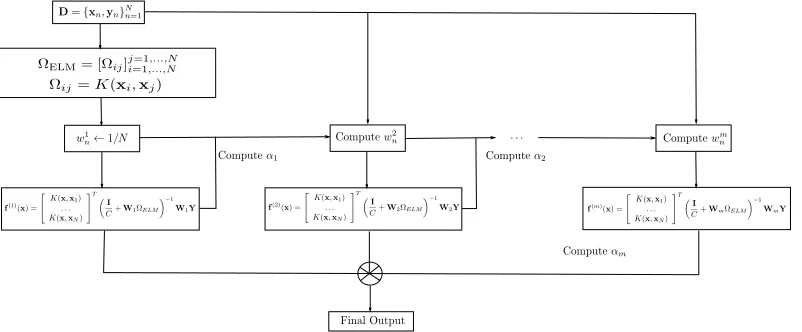
Fig. 2: AdaBoost(ELM) training algorithm framework

Fig. 3: Graphical illustration of the AdaBoost(ELM)

where Wis a diagonal matrix of dimensionN ×N defined 1

as: 2

W =



  

w1 0 . . . 0 0 w2 . . . 0

. . . .

0 . . . 0 wN



  

∈RN ×RN. (17)

The optimalβvalue is computed as critical point of the first order derivative of the weighted error function, hence solution of the following linear system

∂ ∂β

(Hβ−Y)TW(Hβ−Y)

= 0

∂ ∂β

h

(βTHTWHβ−βTHTWY−YTWHβ+

+YTWY)

= 0

(HTWHβ)T+βTHTWH−(HTWY)T −YTWH= 0

2βTHTWH−2YTWH= 0.

Finally, the weighted least squares solution can be approx-3

imate by the generalized form: 4

ˆ

β=

(

HT I

C+WHH

T−1

WY forN < S, I

C +H

T_WH−1_HT_{WY otherwise.} (18)

The output function of them-th ELM classifier is defined as (just for the case N < S)

f(m)(x) =h(x)βˆ

=h(x)HT

_I

C +WHH

T

−1

WY, (19)

where h(x) is a mapping function that corresponds to the basis functions outputs in the neural network literature or it is unknown to users in the kernel machines literature. Therefore, the output function can be kernelized, as suggested in [44], as

f(m)(x) =K(x)T

_I

C +WΩELM

−1

where K(x) : _RK _→

RN is the vector of kernel functions

1

K(x)T _{= [K(x,x}

1), . . . , K(x,xN)]. The Gaussian kernel 2

function here considered is 3

K(x,xi) = exp(−k||x−xi||2), i= 1, . . . , N (21)

where k ∈ R is the kernel parameter. Similarly the kernel

4

matrixΩELM= [Ωi,j]i,j=1,...,N is defined element by element 5

as 6

Ωi,j =K(xi,xj). (22)

The algorithm proposed is named AdaBoost based on ELM 7

(AdaBoost(ELM)) and is described in Fig. 2 and Fig. 3. 8

To tackle Ordinal Regression problems the AdaBoost(ELM) 9

algorithm has been extended to include the cost model intro-10

duced in Section III. In particular three new algorithms are 11

generated, namely AdaBoost for Ordinal Regression based 12

on ELM and Cost model i (AdaBoost(ELM).ORC[i]), with 13

i= 1,2,3. They differ from the algorithm in Figure 2 in the 14

update schema of the error estimation and/or of the patterns 15

weights. In particular the following modifications apply 16

• AdaBoost(ELM).ORC1:

6 :e(m)←

PN

n=1κ (m)

n wn(m)I(o(m)(xn)6=cn)

PN

n=1κ (m)

n w

(m)

n

• AdaBoost(ELM).ORC2:

8 :w(_nm+1)←w_n(m)exp(κ(_nm)α(m)I(o(m)(xn)6=cn))

∀n= 1, . . . , N

• AdaBoost(ELM).ORC3:

6 :e(m)←

PN

n=1κ (m)

n wn(m)I(o(m)(xn)6=cn)

PN

n=1κ (m)

n w

(m)

n

8 :w(_nm+1)←w_n(m)exp(κ_n(m)α(m)I(o(m)(xn)6=cn))

∀n= 1, . . . , N

where κ(nm) is the cost factor computed as described in 17

Section III. 18

V. EXPERIMENTALFRAMEWORK 19

In this section, the experimental study performed to validate 20

the new algorithms is presented. In Section V-A details of the 21

datasets selected for the experimentation are provided. Section 22

V-B gives the measures employed to evaluate the performance 23

of the algorithms. Instead, Section V-C is dedicated to a de-24

scription of the algorithms chosen for the comparison and their 25

relevant parameters. Finally, the description of the statistical 26

tests used to validate the obtained results (see Section V-D) is 27

provided. 28

A. Ordinal regression datasets 29

Sixteen datasets have been selected from the UCI [51] and 30

the mldata.org repositories and one synthetic dataset (the toy 31

dataset) has been included in the test sets. The latter dataset 32

was created as suggested in [52]: 300 example patterns x= 33

(x1, x2)were generated uniformly at random in the unit square

34

[0,1]×[0,1] ⊂ _R2_{. To each pattern a class y from the set}

35

{C1,C2,C3,C4,C5} has been assigned according to:

36

O(y) = min{j:θj−1<10(x1−0.5)(x2−0.5) +ε < θj}

where O(y) represents the rank of the patterns, θj is the threshold for thej-th class, according to the values

(θ0, θ1, θ2, θ3, θ4, θ5) = (−∞,−1,−0.1,0.25,1,∞),

andε∼N(0; 0.1252_{)simulates the possible existence of error}

37

in the assignment of the true class to x. 38

TABLE II: Characteristics of the sixteen datasets used for the experiments: number of patterns (Size), total number of inputs (#In.), number of classes (#Out.), and number of patterns per-class (NPPC)

Dataset Size #In.#Out. NPPC

ERA 1000 4 9 (92,142,181,172,158,118,88,31,18) ELS 488 4 9 (2,12,38,100,116,135,62,19,4) LEV 1000 4 5 (93,280,403,197,27) SWD 1000 10 4 (32,352,399,217) automobile 205 71 6 (3,22,67,54,32,27) balance-scale 625 4 3 (288,49,288)

car 1728 21 4 (1210,384,69,65) contact-lenses 24 6 3 (15,4,4)

eucalyptus 736 91 5 (180,107,130,214,105) newthyroid 215 5 3 (30,150,35)

pasture 36 25 3 (12,12,12) squash-stored 52 51 3 (23,21,8) squash-unstored 52 52 3 (24,24,4)

tae 151 54 3 (49,50,52)

toy 300 2 5 (35,87,79,68,31) winequality-red 1599 11 6 (10,53,681,638,199,19)

Table II summarizes the properties of the selected datasets. 39

It shows, for each dataset, the number of patterns (Size), 40

the total number of inputs (#In.), the number of classes 41

(#Out.) and the number of patterns per-class (NPPC). Their 42

descriptions (available in the web sites) lead to the conclusion 43

that they are ordinal datasets since the class labels show an 44

ordinal nature. 45

The datasets considered are partitioned by using a hold-out 46

cross-validation procedure. Concretely, 30 different stratified 47

random splits of the datasets have been considered, with 48

75% and 25% of the instances in the training and test sets 49

respectively (30 hold-outs). 50

B. Performance measures for Ordinal Regression 51

In this study, ordinal regression datasets are considered. 52

In these domains, two measures are widely used because 53

of their simplicity and successful application. Therefore, 54

two evaluation metrics have been considered which quan-55

tify the accuracy of N predicted ordinal labels for a given 56

dataset {y1,ˆ y2, . . . ,ˆ yˆN}, with respect to the true targets 57

{y1, y2, . . . , yN}. Namely they are: 58

• Accuracy rate (Acc): It is the number of successful hits 59

(correct classifications) relative to the total number of 60

TABLE III: Parameter specification for the methods considered (C: regularization parameter; k: width of the Gaussian functions;M: number of models in the ensemble;S: number of basis functions). The criteria for selecting the best configuration was theM AE performance

Algorithm Ref. Parameters

ASAOR [23] There is no hyperparameters to be considered

MCOSvm [24] C: Best∈ {103_,102_{, . . . ,10}−3_{};k: Best∈ {10}3_,102_{, . . . ,10}−3_{}; Gaussian Kernel} ORBoost-All [29] M= 25;SBest∈ {5,10,15,20,30,40}; Sigmoidal Basis Function

ORBoost-LR [29] M= 25;SBest∈ {5,10,15,20,30,40}; Sigmoidal Basis Function ELMOR [53] SBest∈ {10 +i10},i= 0, . . . ,19; Sigmoidal Basis Function

AdaBoost(ELM) - M= 25;C: Best∈ {103_,102_{, . . . ,10}−3_{};k: Best∈ {10}3_,102_{, . . . ,10}−3_{}; Gaussian Kernel} AdaBoost(ELM).ORC1 - M= 25;C: Best∈ {103_,102_{, . . . ,10}−3_{};k: Best∈ {10}3_,102_{, . . . ,10}−3_{}; Gaussian Kernel} AdaBoost(ELM).ORC2 - M= 25;C: Best∈ {103_,102_{, . . . ,10}−3_{};k: Best∈ {10}3_,102_{, . . . ,10}−3_{}; Gaussian Kernel} AdaBoost(ELM).ORC3 - M= 25;C: Best∈ {103_,102_{, . . . ,10}−3_{};k: Best∈ {10}3_,102_{, . . . ,10}−3_{}; Gaussian Kernel}

used metric to assess the performance of classifiers for 1

years [3]. The mathematical expression ofAcc is: 2

Acc= 1

N

N

X

n=1

I(ˆyn=yn), (23)

where I(·) is the zero-one loss function and N is the 3

number of patterns of the dataset. 4

• Mean Absolute Error (M AE): It is the average devia-5

tion of the prediction from the true targets, i.e.: 6

M AE= 1

N

N

X

n=1

|O(ˆyn)− O(yn)|, (24)

where O(Cj) =j,1≤j ≤J, i.e.O(yn)is the rank of 7

pattern xn according to the encoding scheme used. 8

These measures aim to evaluate different aspects that can 9

be taken into account when an ordinal regression problem is 10

considered: (a)Acc measures that patterns are generally well 11

classified, and (b)M AE measures that the classifier tends to 12

predict a class as closely as possible to the real class without 13

taking into account the relative sizes of the classes. 14

Additionally, the time required to estimate the parameters 15

of each method has been also considered. The time (T) is the 16

simplest way to measure the practical efficiency of a method. 17

The average time elapsed (in seconds) is analyzed by every 18

method, considering cross-validation time, training and test 19

time. 20

C. Comparison Methods 21

The models proposed have been evaluated comparing their 22

results to the results of ensemble models for ordinal regression 23

and one extreme learning approach for ordinal data. All of 24

them have been already mentioned in the Introduction section. 25

• Ensemble approaches for Ordinal regression: 26

– A Simple Approach to Ordinal Regression

27

(ASAOR)[23] is a meta classifier that allows stan-28

dard classification algorithms to be applied to ordinal 29

class problems. In the current work, the C4.5 method 30

available in Weka [54] is used as the underlying 31

classification algorithm, since this is the one initially 32

employed by the authors. 33

– Multi-Class Ordinal Support vector machines

34

(MCOSvm) [24] is an enhanced ensemble method 35

for ordinal regression. As proposed in [24], weighted 36

SVMs are used as base classifiers. Specific weights 37

are assigned to each pattern in such a way that 38

errors of more than one rank are heavier penalized. 39

Therefore the weight of a training pattern differs for 40

each binary SVM. 41

– Ordinal Regression Boosting (ORBoost) [29] is 42

a thresholded ensemble model for ordinal regres-43

sion problems. The model consists of a weighted 44

ensemble of confidence functions and an ordered 45

vector of thresholds. ORBoost can be used with 46

any base learners for confidence functions. In the 47

presented experimental study, a standard feedforward 48

neural network is used as the underlying classifica-49

tion model. Two boosting approaches are considered: 50

∗ ORBoost with all margins (ORBoost-All). 51

∗ ORBoost with left-right margins (ORBoost-LR). 52

• ELM models for Ordinal regression: 53

– Extreme Learning Machine for Ordinal

Regres-54

sion (ELMOR) [53]. For this experimental study 55

the single model proposed in [53] is employed. The 56

other two multiple model approaches have not been 57

considered for efficiency reasons. 58

Table III presents the parameters configuration of the dif-59

ferent models proposed. In the case of ensemble models the 60

same size has been considered for all the methods M = 25. 61

However, for the iterative neural network ensemble algorithms 62

(ORBoost.LR and ORBoost.All), the number of basis func-63

tions S, were selected by considering the following values, 64

S ∈ {5,10,20,30,40} while for the ordinal ELM algorithm 65

(ELMOR), it is necessary to consider a more extensive set of 66

possible number of basis functions, in this caseS ∈ {10+i10}

67

with i = 0, . . . ,19, given that the method relies on random 68

projections. For the ensemble kernel methods (MCOSvm and 69

AdaBoost(ELM) algorithm and its ordinal variants), the regu-70

larization parameter,C, and the width of the Gaussian kernel, 71

k, were selected by considering the following set of values, 72

C andk ∈ {103,102, . . . ,10−3}. The hyperparameters were 73

adjusted using a grid search with a 5-fold cross-validation 74

considering just the training set. Despite this, the optimal 75

number of basis functions for the ELMOR could be also 76

D. Statistical Tests for Performance Comparison 1

In the presented experimental study, the hypothesis testing 2

techniques are used to provide statistical support for the 3

analysis of the results. Concretely, nonparametric tests have 4

been used, due to the fact that the initial conditions that 5

guarantee the reliability of the parametric tests may not be 6

satisfied, causing the statistical analysis to lose credibility [56]. 7

Throughout the study, the Friedman test is used to detect 8

statistical differences among the methods. Holmpost hoc pro-9

cedure will be used to find out which methods are distinctive 10

among the multiple comparisons performed [56]. 11

VI. RESULTS ANDANALYSIS 12

In this section, the different experimental studies carried 13

out with the cost-sensitive boosting proposals are detailed. In 14

particular, the aims are multiple: 15

1) To compare the generalization performance of the ap-16

proaches proposed to recent ensemble and ELM algo-17

rithms for ordinal regression (Section VI-A). 18

2) To test the time complexity of the models proposed 19

compared to the above-mentioned methods (Section 20

VI-B). 21

3) To show the influence of the hyperparameters in the 22

overall performance (Section VI-C) 23

A. Comparison between the models proposed and ensemble 24

and ELM algorithms for ordinal regression 25

For the sake of simplicity, only the graphical and the sum-26

mary of the statistical results achieved are included, whereas 27

the complete results can be found online2_. 28

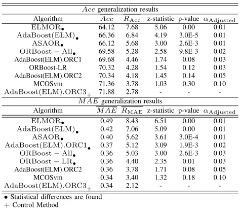
TABLE IV: Summary of results in Acc and M AE for the generalization set: Mean results over all the datasets, mean ranking and Holm statistical test results (using as the control method the one with the best mean ranking) for α= 0.10

Accgeneralization results

Algorithm Acc RAcc z-statistic p-value αAdjusted

ELMOR• 64.12 7.68 5.06 0.00 0.01

AdaBoost(ELM)_• 66.36 6.84 4.19 3.0E-5 0.01

ASAOR• 66.12 5.68 3.00 2.6E-3 0.01

ORBoost−All• 69.58 5.28 2.58 9.8E-3 0.02

AdaBoost(ELM).ORC1 69.68 4.46 1.74 0.08 0.03 ORBoost-LR 70.32 4.28 1.54 0.12 0.03 AdaBoost(ELM).ORC2 70.34 4.18 1.45 0.14 0.05 MCOSvm 71.36 3.78 1.03 0.30 0.10

AdaBoost(ELM).ORC3₊ 71.88 2.78 - - -M AEgeneralization results

Algorithm M AE RMAE z-statistic p-value αAdjusted

ELMOR• 0.49 8.43 6.51 0.00 0.01

AdaBoost(ELM)_• 0.42 7.06 5.09 0.00 0.01

ASAOR• 0.40 5.62 3.61 3.0E-4 0.01

AdaBoost(ELM).ORC1_• 0.37 5.12 3.09 1.9E-3 0.02

ORBoost−All• 0.36 5.03 3.00 2.6E-3 0.03

ORBoost−LR• 0.36 4.40 2.35 0.01 0.03

AdaBoost(ELM).ORC2 0.36 3.78 1.71 0.08 0.05 MCOSvm 0.34 3.40 1.32 0.18 0.10

AdaBoost(ELM).ORC3₊ 0.34 2.12 - -

-•Statistical differences are found

+Control Method

Fig. 4 is the star plot representation of generalization 29

performance of the comparison of the different methodologies. 30

2_{http://www.esa.int/gsp/ACT/cms/projects/ResultsAdaboostELM.zip}

This star plot represents the performance as the distance from 31

the center; hence a higher area determines the best average 32

performance where the goal is to maximize the metric (Acc) 33

and lower area determines the best average performance where 34

the goal is to minimize (M AE). The plot allows to visualize 35

the performance of the algorithms comparatively for each 36

dataset. As can be seen in Fig. 4, the AdaBoost(ELM).ORC3 is 37

the most promising methodology following by the MCOSvm 38

method. From the analysis of the results (Table IV), it can 39

be concluded that the AdaBoost(ELM).ORC3 model produces 40

the best mean ranking in Acc and M AE (RAcc = 2.78 and 41

RMAE = 2.12), reporting also the best mean accuracy and 42

mean absolute error (Acc= 71.88% andM AE = 0.34). 43

To determine the statistical significance of the rank differ-44

ences observed for each method in the different datasets, a 45

non-parametric Friedman test [57] has been completed with 46

the ranking ofAccandM AE in the generalization set of the 47

best models as test variables. The test shows that the effect of 48

the method used for classification is statistically significant at 49

a significance level of10%. 50

Based on this rejection, the Holm post-hoc test was used 51

to compare all classifiers with a control method [58]. For the 52

experiments carried out, the control method selected is the 53

one reporting the best mean ranking in Acc and M AE, the 54

AdaBoost(ELM).ORC3. The results of the Holm test forα= 55

0.10can be seen in Table IV. By using a level of significance 56

α= 0.10, AdaBoost(ELM).ORC3 is significantly better than 57

ELMOR, AdaBoost(ELM), ASAOR and ORBoost-All using 58

Acc as variable test, and significantly better than ELMOR, 59

AdaBoost(ELM), ASAOR, AdaBoost(ELM).ORC1, ORBoost-60

All and ORBoost-LR using M AE as variable test. 61

As can be seen in Table IV, the AdaBoost(ELM).ORC3 62

algorithm is competitive when compared to the most promising 63

ensemble methods for ordinal regression. Furthermore, it is 64

much more efficient than most of them. This justifies its 65

proposal. 66

B. Time complexity analysis 67

In this section, the computational time and complexity of 68

the proposed methods are analyzed and compared to the al-69

ready existing ensemble models for ordinal regression already 70

presented in the experimental section. 71

The computational complexity of the SAMME algorithm is 72

conditioned by the choice of its base classifier. In the proposed 73

ELM model the computation of the kernel matrix has a 74

quadratic complexity inN, whereN is the size of the dataset. 75

However the kernel matrix is initialized at the beginning of 76

the ensemble and not recomputed. In each iteration of model, 77

the most time consuming task is the inversion of a N ×N

78

matrix and the multiplication of it with a matrix of dimension 79

N×J. The computational complexity of the multiplication of 80

the two matrices isO(N2J), while the complexity of inverting 81

the matrix of dimension N is O(N3) (if the Gauss–Jordan 82

elimination algorithm is used), where N is the number of 83

training patterns and J is the number of classes. Hence the 84

computational complexity of the AdaBoost(ELM) algorithm is 85

O((N3_+N2_{J)M), whereM is the size of its ensemble [31].}

0 10 20 30 40 50 60 70 80 90 100 ERA

ESL

LEV

SWD

automobile

balance-scale

car

contact-lenses eucalyptus

newthyroid pasture squash-stored squash-unstored

tae toy

winequality-red AdaBoost(ELM)

AdaBoost(ELM).ORC1 AdaBoost(ELM).ORC2 AdaBoost(ELM).ORC3

(a)Accresults: Comparison to AdaBoost models

0 0.2 0.4 0.6 0.8 1 1.2 1.4 1.6

AdaBoost(ELM) AdaBoost(ELM).ORC1 AdaBoost(ELM).ORC2 AdaBoost(ELM).ORC3

(b)M AEresults: Comparison to AdaBoost models

0 10 20 30 40 50 60 70 80 90 100 ERA

ESL

LEV

SWD

automobile

balance-scale

car

contact-lenses eucalyptus

newthyroid pasture squash-stored squash-unstored

tae toy winequality-red

ASAOR MCOSvm ORBoost-All ORBoost-LR ELMOR AdaBoost(ELM).ORC3

(c)Accresults: AdaBoost(ELM).ORC3 versus state-of-the-art models

0 0.2 0.4 0.6 0.8 1 1.2 1.4 1.6

ERA

ESL

LEV

SWD

automobile

balance-scale

car

contact-lenses eucalyptus

newthyroid pasture squash-stored squash-unstored

tae toy winequality-red

ASAOR MCOSvm ORBoost-All ORBoost-LR ELMOR AdaBoost(ELM).ORC3

(d)M AEresults: AdaBoost(ELM).ORC3 versus state-of-the-art models Fig. 4: Radar illustration of the results onAcc(Figure 4a and 4c) and M AE (Figure 4b and 4d)

The time recorded included cross-validation, training and 1

test, and it is shown in Table V. The number of hyperparam-2

eters of each method is decisive for the final time spent in 3

running the algorithms, given that they have to be adjusted 4

using a time-consuming cross-validation process (see Section 5

V-C for further details). 6

TABLE V: Computational time results in seconds (cross-validation, training and test) for the toy dataset and all the methods: average and standard deviation over the30holdouts.

Computational Time (M eanSD)

ORBoost-All 216.92 (160.54)

ORBoost-LR 215.92 (76.35)

MCOSvm 27.4 (0.90)

AdaBoost(ELM).ORC1 10.6 (0.5)

AdaBoost(ELM).ORC2 10.6 (0.5)

AdaBoost(ELM).ORC3 10.5 (0.3)

AdaBoost(ELM) 10.4 (0.4)

ELMOR 1.2 (0.6)

ASAOR 0.15 (0.04)

As can be seen, the ensemble models proposed are the 7

methods with the lowest computational time, together with 8

MCOSvm, ELMOR and ASAOR. The differences in time 9

of these methods are not significant if they are compared 10

to the differences with the ORBoost-All and ORBoost-LR 11

methods. A simplified version of the proposed ensemble 12

model, with a neural network as base classifier and without the 13

regularization parameter and the kernel functions, has a single 14

hyperparameter to be tuned (the number of hidden nodes) and 15

doesn’t require the computation of the kernel matrix. This 16

results in a more computational efficient model (is gained 17

approximately one order of magnitude) but less performing. 18

For this reason, the base classifier with its kernel version and 19

with the regularization parameter is the one proposed in this 20

paper. 21

Furthermore, note that software implementations can affect 22

these times. For example, the ASAOR Weka implementation 23

was written in Java and the remaining methods were run using 24

a common Matlab framework proposed in Gutierrez et al. [59]. 25

In general, the most efficient algorithms are the ones based 26

on ELM. Both are trained without iterative tuning. Despite 27

this, the lowest computation time is achieved by the ASAOR 28

not any hyperparameters to be optimized by cross-validation 1

unlike ELMOR and AdaBoost(ELM) approaches (they have, 2

respectively, the number of basis functions S, and the kernel 3

and regularization parameters(C, k)as hyperparameters). The 4

efficiency of the models proposed and their good performance 5

justify their proposal. 6

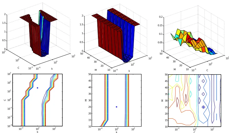
C. Influence of the hyperparameters 7

The proposed algorithms rely on three hypeparameters that 8

need to be set: the size of the ensemble M, the regularization 9

coefficient, C and the width of the Gaussian kernel k. A 10

study has been performed to analyze the sensitivity of the 11

model, in terms of Accuracy and M AE, with respect to the 12

three hyperparameters. The algorithm considered is the one 13

achieving the best results, AdaBoost(ELM).ORC3, on the toy 14

problem. The hyperparameters are compared 2-by-2 fixing the 15

value of the third one to the best value achieved in the cross 16

validation process. In particular the best set of values used in 17

this particular case is 18

(M∗, C∗, k∗) = (25,10,1). (25)

While (C∗, k∗) are result of the cross-validation process,

M∗ = 25 has been considered as competitive trade-off between efficiency, diversity and accuracy [60]. Several runs of the AdaBoost(ELM).ORC3 model have been performed for values of the three hyperparameters ranging in the sets

M ∈ {10, . . . ,50}

C, k∈ {10−3, . . . ,103}. (26)

Results are reported in Fig. 5 and Fig. 6, where also the 19

solution of the cross validation process is drawn in the contour 20

lines plot for comparison. As expected the model is less 21

sensitive to the size of its ensemble: the significant variations 22

in performance are determined by the (C, k)parameters. The 23

most critical parameter is the width of the Gaussian kernelk. 24

The accuracy of the model has a very sensitive behavior with 25

respect to the parameter k, with a drop down up to 80% of 26

the overall model performance. 27

VII. CONCLUSIONS 28

The presented work extends the class of boosting algorithms 29

for ordinal regression. In particular it enlarges the family of 30

models that employ Extreme Learning Machine (ELM) as a 31

base classifier. It differs from the already existing techniques 32

in the way of addressing the training at each iteration of the 33

ensemble. Instead of generating at each step a new training 34

dataset according to the new set of patterns weights, the 35

weights are used into the definition of the training problem, 36

solving the derived Weighted Least Squares Problem (WLSP) 37

in a close form and maintain the original training dataset 38

during all the iterations cycle. Moreover, in order to be 39

applied to Ordinal Regression problems, three cost models 40

have been proposed that affect the way in which the weights 41

are redistributed among the patterns. 42

After introducing the existing boosting algorithms, in par-43

ticular those using ELM as base classifier, more attention has 44

been given to the description of the Stagewise Additive Mod-45

eling using a Multi-class Exponential loss function (SAMME) 46

algorithm, being the version of the AdaBoost method adopted 47

in the proposed algorithms. The SAMME algorithm has been 48

extended, in order to address ordinal regression problems, 49

including three cost models and using an ELM as base classi-50

fier that determines the linear parameters of the kernel ELM 51

method using the analytic solution of the WLSP. This led to 52

the definition of four new algorithms, namely AdaBoost(ELM) 53

for nominal classification and AdaBoost(ELM).ORC1, Ad-54

aBoost(ELM).ORC2 and AdaBoost(ELM).ORC3 for ordinal 55

regression. 56

Ordinal regression datasets available in the community and 57

one synthetic dataset (the toy dataset) have been used as 58

benchmark test sets, four algorithms from the state-of-the-art 59

ensemble models for ordinal regression (ASAOR, MCOSvm, 60

ORBoost-All, ORBoost-LR) and one extreme learning ap-61

proach for ordinal data (ELMOR) have been used for compar-62

ison and the model performance has been evaluated using the 63

Accuracy and Mean Absolute Error (M AE) measures. Finally 64

the models have been compared also in terms of computational 65

efficiency, non parametric statistical tests have been performed 66

to validate the results and an analysis of the influence of 67

the hyperparameters on the selected metrics has also been 68

included. 69

From the results of these tests the AdaBoost(ELM).ORC3 70

algorithm is the method, among the one proposed in this 71

article, with the most effective cost model. The algorithm 72

reaches competitive results in terms of performance with the 73

state of the art ensemble models, achieving the best mean 74

ranking in accuracy and in mean absolute error. Furthermore, 75

the models proposed outperforms in efficiency the selected 76

ensemble models for ordinal regression but the ASAOR algo-77

rithm. It’s comparable performances with the state-of-the-art 78

algorithms and its efficiency justify its proposal. 79

The adaptation of the algorithms proposed to the incre-80

mental learning paradigm will be considered as future work. 81

Indeed the Adaboost algorithm has already been adapted to the 82

incremental learning paradigm [61] for nominal classification 83

[62], [63] but not for ordinal regression problems. 84

REFERENCES 85

[1] A. K. Jain, R. P. Duin, and J. Mao, “Statistical pattern recognition: A re-86

view,”IEEE Transactions on Pattern Analysis and Machine Intelligence, 87

vol. 22, no. 1, pp. 4–37, 2000. 88

[2] R. O. Duda, P. E. Hart, and D. G. Stork,Pattern Classification, 2nd ed. 89

Wiley-Interscience, 2000. 90

[3] I. H. Witten and E. Frank,Data Mining: Practical Machine Learning 91

Tools and Techniques, 2nd ed., ser. Data Management Systems. Morgan 92

Kaufmann (Elsevier), 2005. 93

[4] V. Cherkassky and F. M. Mulier,Learning from Data: Concepts, Theory, 94

and Methods. Wiley-Interscience, 2007. 95

[5] B.-Y. Sun, J. Li, D. D. Wu, X.-M. Zhang, and W.-B. Li, “Kernel 96

discriminant learning for ordinal regression,” IEEE Transactions on 97

Knowledge and Data Engineering, vol. 22, no. 6, pp. 906–910, 2010. 98

[6] C.-W. Seah, I. W. Tsang, and Y.-S. Ong, “Transductive ordinal regres-99

sion,” IEEE Transactions on Neural Networks and Learning Systems, 100

vol. 23, no. 7, pp. 1074–1086, 2012. 101

[7] P. McCullagh, “Regression models for ordinal data,” Journal of the 102

Royal Statistical Society. Series B (Methodological), vol. 42, no. 2, pp. 103

10−5

100

105

10−5

100

1005

20 40 60 80 100

k C

k

C

10−2 ₁₀0 ₁₀2

10−3

10−2

10−1

100

101

102

103

10−5

100

105

10 20 30 40 50

0 20 40 60 80 100

k M

k

M

10−2 ₁₀0 ₁₀2

10 15 20 25 30 35 40 45 50

10−5

100

105

10 20 30 40 50 86 88 90 92 94 96 98 100

C M

AdaBoost.ORC3 Accuracy

C

M

10−2 ₁₀0 ₁₀2

10 15 20 25 30 35 40 45 50

Fig. 5: Hypeparameters study on Acc for the AdaBoost(ELM).ORC3 algorithm and the parameters: M (ensemble size), C

(regularization coefficient), k (width of the Gaussian kernel).

10−5

100

105

10−5

100

1005

0.5 1 1.5 2

k C

k

C

10−2 ₁₀0 ₁₀2

10−3

10−2

10−1

100

101

102

103 10

−5

100

105

10 20 30 40

500

0.5 1 1.5 2

k M

k

M

10−2 ₁₀0 ₁₀2

10 15 20 25 30 35 40 45 50

10−5

100

105

10 20 30 40

500

0.05 0.1 0.15 0.2

C M

AdaBoost.ORC3 Mean Absolute Error

C

M

10−2 ₁₀0 ₁₀2

10 15 20 25 30 35 40 45 50

Fig. 6: Hypeparameters study on M AE for the AdaBoost(ELM).ORC3 algorithm and the parameters:M (ensemble size),C

(regularization coefficient), k (width of the Gaussian kernel).

[8] J. A. Anderson, “Regression and ordered categorical variables,”Journal 1

of the Royal Statistical Society. Series B (Methodological), vol. 46, no. 1, 2

pp. 1–30, 1984. 3

[9] M. J. Mathieson, “Ordinal models for neural networks,” inProceedings 4

of the Third International Conference on Neural Networks in the Capital 5

Markets, ser. Neural Networks in Financial Engineering, J. M. A.-P. 6

N. Refenes, Y. Abu-Mostafa and A. Weigend, Eds. World Scientific, 7

1996, pp. 523–536. 8

[10] F. Fern´andez-Navarro, P. Campoy, M. De la Paz, C. Herv´as-Mart´ınez, 9

and X. Yao, “Addressing the EU sovereign ratings using an ordinal 10

regression approach,”IEEE Transaction on Cybernetics, vol. 43, no. 6, 11

pp. 2228–2240, 2013. 12

[11] R. Herbrich, T. Graepel, and K. Obermayer, “Large margin rank bound-13

aries for ordinal regression,” inAdvances in Large Margin Classifiers, 14

A. Smola, P. Bartlett, B. Sch¨olkopf, and D. Schuurmans, Eds. Cam-15

bridge, MA: MIT Press, 2000, pp. 115–132. 16

[12] W. Chu and S. S. Keerthi, “Support Vector Ordinal Regression,”Neural 17

Computation, vol. 19, no. 3, pp. 792–815, 2007. 18

[13] W. Chu and Z. Ghahramani, “Gaussian processes for ordinal regression,” 19

J. Mach. Learn. Res., vol. 6, pp. 1019–1041, Dec. 2005. 20

[14] W. Deng and L. Chen, “Color image watermarking using regularized 21

extreme learning machine,”Neural Network World, vol. 20, no. 3, pp. 22

317–330, 2010. 23

[15] D. Becerra-Alonso, M. Carbonero-Ruz, F. J. Mart´ınez-Estudillo, and 24

A. C. Mart´ınez-Estudillo, “Evolutionary extreme learning machine for 25

in Computer Science, 2012, vol. 7665, pp. 217–227. 1

[16] Q.-Y. Zhu, A. K. Qin, P. N. Suganthan, and G.-B. Huang, “Evolutionary 2

extreme learning machine,”Pattern Recognition, vol. 38, no. 10, pp. 3

1759–1763, 2005. 4

[17] Y. Liu, X. Yao, and T. Higuchi, “Ensembles with negative correlation 5

learning,” IEEE Transactions on Evolutionary Computation, vol. 4, 6

no. 4, pp. 380–387, 2000. 7

[18] A. Chandra and X. Yao, “Divace: Diverse and accurate ensemble 8

learning algorithm,” inProceedings of the Fifth International Conference 9

on intelligent Data Engineering and Automated learning, vol. 3177. 10

Exeter, UK: Lectures Notes and Computer Science, Springer, Berlin, 11

2005, pp. 619–625. 12

[19] X. Zhu, P. Zhang, X. Lin, and Y. Shi, “Active learning from stream 13

data using optimal weight classifier ensemble,”IEEE Transactions on 14

Systems, Man, and Cybernetics, Part B: Cybernetics, vol. 40, no. 6, pp. 15

1607–1621, 2010. 16

[20] D. Hernandez-Lobato, G. Martinez-Mu??oz, and A. Suarez, “Empirical 17

analysis and evaluation of approximate techniques for pruning regression 18

bagging ensembles,”Neurocomputing, vol. 74, no. 12-13, pp. 2250 – 19

2264, 2011. 20

[21] A. L. Coelho and D. S. Nascimento, “On the evolutionary design of 21

heterogeneous bagging models,” Neurocomputing, vol. 73, no. 16-18, 22

pp. 3319 – 3322, 2010. 23

[22] Z. Qi, Y. Xu, L. Wang, and Y. Song, “Online multiple instance boosting 24

for object detection,”Neurocomputing, vol. 74, no. 10, pp. 1769 – 1775, 25

2011. 26

[23] E. Frank and M. Hall, “A simple approach to ordinal classification,” in 27

ECML’01, 2001, pp. 145–156. 28

[24] W. Waegeman and L. Boullart, “An ensemble of weighted support vector 29

machines for ordinal regression,” International Journal of Computer 30

Systems Science and Engineering, vol. 3, no. 1, pp. 47–51, 2009. 31

[25] F. Fern´andez-Navarro, P. Gutierrez, C. Herv´as-Mart´ınez, and X. Yao, 32

“Negative correlation ensemble learning for ordinal regression,”IEEE 33

Transaction on Neural Networks and Learning Systems, vol. 24, no. 11, 34

pp. 1836–1849, 2013. 35

[26] Y. Liu and X. Yao, “Negatively correlated neural networks can produce 36

best ensembles,”Australian Journal of Intelligent Information Process-37

ing Systems, vol. 4, no. 3, pp. 176–185, 1997. 38

[27] ——, “Ensemble learning via negative correlation,” Neural Networks, 39

vol. 12, no. 10, pp. 1399–1404, 1999. 40

[28] M. P´erez-Ortiz, P. Guti´errez, and C. Herv´as-Mart´ınez, “Projection-41

based ensemble learning for ordinal regression,”IEEE Transactions on 42

Cybernetics, vol. PP, no. 99, pp. 1–1, 2013. 43

[29] H.-T. Lin and L. Li, “Large-margin thresholded ensembles for ordinal 44

regression: theory and practice,” inProceedings of the 17th international 45

conference on Algorithmic Learning Theory, ser. ALT’06. Springer-46

Verlag, 2006, pp. 319–333. 47

[30] ——, “Combining ordinal preferences by boosting,” inProceedings of 48

the ECML/PKDD 2009, ser. Workshop on Preference Learning, 2009, 49

pp. 69–83. 50

[31] J. Zhu, H. Zou, S. Rosset, and T. Hastie, “Multi-class adaboost,” 51

Statistics and Its Interface, vol. 2, no. 1, pp. 349–360, 2009. 52

[32] R. E. Schapire and Y. Singer, “Improved boosting algorithms using 53

confidence-rated predictions,” Machine Learning, vol. 37, no. 3, pp. 54

297–336, 1999. 55

[33] G.-B. Huang, D. Wang, and Y. Lan, “Extreme learning machines: a 56

survey,”International Journal of Machine Learning and Cybernetics, 57

vol. 2, no. 2, pp. 107–122, 2011. 58

[34] G. Wang and P. Li, “Dynamic adaboost ensemble extreme learning 59

machine,” inAdvanced Computer Theory and Engineering (ICACTE), 60

2010 3rd International Conference on, vol. 3, 2010, pp. V3–54–V3–58. 61

[35] H.-X. Tian and Z.-Z. Mao, “An ensemble elm based on modified 62

adaboost.rt algorithm for predicting the temperature of molten steel in 63

ladle furnace,”Automation Science and Engineering, IEEE Transactions 64

on, vol. 7, no. 1, pp. 73–80, 2010. 65

[36] J.-H. Zhai, H.-Y. Xu, and X.-Z. Wang, “Dynamic ensemble extreme 66

learning machine based on sample entropy,”Soft Computing, vol. 16, 67

no. 9, pp. 1493–1502, 2012. 68

[37] Y. Sun, M. S. Kamel, A. K. C. Wong, and Y. Wang, “Cost-sensitive 69

boosting for classification of imbalanced data,” Pattern Recognition, 70

vol. 40, no. 12, pp. 3358–3378, 2007. 71

[38] H.-T. Lin and L. Li, “Reduction from cost-sensitive ordinal ranking to 72

weighted binary classification,”Neural Computation, vol. 24, no. 5, pp. 73

1329–1367, 2012. 74

[39] G. B. Huang, Q. Y. Zhu, and C. K. Siew, “Extreme learning machine: 75

A new learning scheme of feedforward neural networks,” in IEEE 76

International Conference on Neural Networks - Conference Proceedings, 77

vol. 2, 2004, pp. 985–990. 78

[40] C. Zhaohu, R. Xuemei, and C. Qiang, “Camera calibration based on 79

extreme learning machine,” in Proceedings of the 2012 International 80

Conference on Communication, Electronics and Automation Engineer-81

ing, ser. Advances in Intelligent Systems and Computing. Springer 82

Berlin Heidelberg, 2013, vol. 181, pp. 115–120. 83

[41] H. Zhou, Y. Lan, Y. C. Soh, G.-B. Huang, and R. Zhang, “Credit 84

risk evaluation with extreme learning machine,” inSystems, Man, and 85

Cybernetics (SMC), 2012 IEEE International Conference on, 2012, pp. 86

1064–1069. 87

[42] J. S´anchez-Monedero, M. Cruz-Ram´ırez, F. Fern´andez-Navarro, J. C. 88

Fern´andez, P. A. Guti´errez, and C. Herv´as-Mart´ınez, “On the suitability 89

of extreme learning machine for gene classification using feature selec-90

tion,” inISDA ’10: Proceedings of the 2010 International Conference 91

on Intelligent Systems Design and Applications. Cairo, Egypt: IEEE 92

Computer Society, 2010, pp. 507–512. 93

[43] G.-B. Huang, Q.-Y. Zhu, and C.-K. Siew, “Extreme learning machine: 94

Theory and applications,”Neurocomputing, vol. 70, no. 1-3, pp. 489 – 95

501, 2006. 96

[44] G.-B. Huang, H. Zhou, X. Ding, and R. Zhang, “Extreme learning 97

machine for regression and multiclass classification,”IEEE Transactions 98

on Systems, Man, and Cybernetics, Part B: Cybernetics, vol. 42, no. 2, 99

pp. 513–529, 2012. 100

[45] V. N. Vapnik,The Nature of Statistical Learning Theory. Springer, 101

1999. 102

[46] R. Zhang, G.-B. Huang, N. Sundararajan, and P. Saratchandran, “Multi-103

category classification using an extreme learning machine for microarray 104

gene expression cancer diagnosis,”IEEE/ACM Transactions on Compu-105

tational Biology and Bioinformatics, vol. 4, no. 3, pp. 485–495, 2007. 106

[47] P. Bartlett, “The sample complexity of pattern classification with neural 107

networks: the size of the weights is more important than the size of the 108

network,”Information Theory, IEEE Transactions on, vol. 44, no. 2, pp. 109

525–536, 1998. 110

[48] J. Cao, Z. Lin, and G.-b. Huang, “Composite function wavelet neural 111

networks with extreme learning machine,”Neurocomputing, vol. 73, no. 112

7-9, pp. 1405–1416, 2010. 113

[49] F. Fern´andez-Navarro, C. Herv´as-Mart´ınez, J. S´anchez-Monedero, and 114

P. A. Gutierrez, “MELM-GRBF: A modified version of the extreme 115

learning machine for generalized radial basis function neural networks,” 116

Neurocomputing, vol. 74, no. 16, pp. 2502–2510, 2011. 117

[50] A. E. Hoerl and R. W. Kennard, “Ridge regression: Biased estimation 118

for nonorthogonal problems,”Technometrics, vol. 12, no. 1, pp. 55–67, 119

1970. 120

[51] A. Asuncion and D. Newman, “UCI machine learning repository,” 2007. 121

[Online]. Available: http://www.ics.uci.edu/∼_{mlearn/MLRepository.html}

122

[52] J. S. Cardoso and J. F. Pinto da Costa, “Learning to classify ordinal 123

data: The data replication method,” J. Mach. Learn. Res., vol. 8, pp. 124

1393–1429, Dec. 2007. 125

[53] W.-Y. Deng, Q.-H. Zheng, S. Lian, L. Chen, and X. Wang, “Ordinal 126

extreme learning machine,”Neurocomputing, vol. 74, no. 1–3, pp. 447– 127

456, 2010. 128

[54] M. Hall, E. Frank, G. Holmes, B. Pfahringer, P. Reutemann, and I. H. 129

Witten, “The WEKA data mining software: an update,”Special Interest 130

Group on Knowledge Discovery and Data Mining Explorer Newsletter, 131

vol. 11, pp. 10–18, November 2009. 132

[55] A. Casta˜no, F. Fern´andez-Navarro, and C. Herv´as-Mart´ınez, “PCA-133

ELM: A robust and pruned extreme learning machine approach based 134

on principal component analysis,”Neural Processing Letters, vol. 37, 135

no. 3, pp. 377–392, 2013. 136

[56] J. Demˇsar, “Statistical comparisons of classifiers over multiple data sets,” 137

J. Mach. Learn. Res., vol. 7, pp. 1–30, Dec. 2006. 138

[57] M. Friedman, “A comparison of alternative tests of significance for the 139

problem of m rankings,”Annals of Mathematical Statistics, vol. 11, 140

no. 1, pp. 86–92, 1940. 141

[58] Y. Hochberg and A. Tamhane,Multiple Comparison Procedures. John 142

Wiley & Sons, 1987. 143

[59] P. A. Guti´errez, M. P´erez-Ortiz, F. Fern´andez-Navarro, J. S´anchez-144

Monedero, and C. Herv´as-Mart´ınez, “An experimental study of different 145

ordinal regression methods and measures,” inHybrid Artificial Intelli-146

gent Systems, ser. Lecture Notes in Computer Science. Springer Berlin 147

Heidelberg, 2012, vol. 7209, pp. 296–307. 148

[60] G. Brown, J. L. Wyatt, and P. Tiˇno, “Managing diversity in regression 149

ensembles,” J. Mach. Learn. Res., vol. 6, pp. 1621–1650, Dec. 2005. 150