City, University of London Institutional Repository
Citation
:
Child, C. H. T. (2011). Approximate Dynamic Programming with ParallelStochastic Planning Operators. (Unpublished Doctoral thesis, City University London)
This is the unspecified version of the paper.
This version of the publication may differ from the final published
version.
Permanent repository link: http://openaccess.city.ac.uk/1109/
Link to published version
:
Copyright and reuse:
City Research Online aims to make research
outputs of City, University of London available to a wider audience.
Copyright and Moral Rights remain with the author(s) and/or copyright
holders. URLs from City Research Online may be freely distributed and
linked to.
1
Department of Computing
Approximate Dynamic Programming with
Parallel Stochastic Planning Operators
Christopher H. T. Child
A thesis submitted for the degree of
Doctor of Philosophy at City University London
3
Contents
1. INTRODUCTION ... 23
1.1 MOTIVATION ... 27
1.2 AIMS &OBJECTIVES ... 28
1.3 FRAMEWORK... 29
1.4 CONTRIBUTIONS ... 29
1.5 STRUCTURE ... 30
1.6 PREVIOUS PUBLICATIONS ... 30
2. BACKGROUND I: AGENTS, ENVIRONMENTS & MODELS ... 33
2.1 AGENTS ... 33
2.1.1 AGENT:ACTION SELECTION WITHIN AN ENVIRONMENT ... 34
2.1.2 AGENT:PERCEIVE,DELIBERATE AND EXECUTE ... 35
2.1.3 ENVIRONMENT UPDATE FUNCTION:DIRECT ACTION,DISCRETE TIME ... 37
2.1.4 EMBODIED AGENTS ... 38
2.2 ENVIRONMENT MODEL ... 41
2.2.1 MARKOV MODELS ... 42
2.2.2 PERCEPTUAL MODEL ... 43
2.3 MODEL REPRESENTATION ... 45
2.3.1 FACTORED STATE MODELS ... 46
2.3.2 INFLUENCE DIAGRAMS ... 48
2.3.3 PROBABILISTIC STRIPS OPERATORS (PSOS) ... 51
2.3.4 NOISY DEICTIC RULES (NDRS) ... 53
2.4 SUMMARY ... 55
4
3.1 MODEL LEARNING ... 57
3.1.1 LEARNING FACTORED STATE MODELS ... 58
3.1.2 LEARNING PSOS WITH THE MSDDALGORITHM ... 60
3.1.3 FILTER ... 62
3.1.4 THE APRIORI ALGORITHM FOR ASSOCIATION RULE MINING ... 64
3.1.5 LEARNING NOISY DEICTIC RULES (NDRS) ... 65
3.2 PLANNING ... 67
3.2.1 REWARD AND VALUE ... 68
3.2.2 SOLUTION METHODS FOR MARKOV DECISION PROCESSES ... 69
3.2.3 REINFORCEMENT LEARNING ... 70
3.2.4 LEARNING RATE ... 71
3.3 SUMMARY ... 72
4. ENVIRONMENT MODELLING AGENT FRAMEWORK ... 73
4.1 INTEGRATED PLANNING,ACTING AND LEARNING ... 73
4.2 BATCH PROCESSED ENVIRONMENT MODELLING AND PLANNING ... 75
4.2.1 STAGE 1:MODEL ENVIRONMENT ... 76
4.2.2 STAGE 2:FORM POLICY ... 77
4.2.3 STAGE 3:EXECUTE POLICY ... 80
4.3 DISCUSSION OF MODEL-BASED REINFORCEMENT LEARNING ... 80
4.4 PERCEPTUAL ENVIRONMENT MODELLING ... 81
4.5 SUMMARY ... 82
5. PARALLEL STOCHASTIC PLANNING OPERATORS: P-SPOS ... 83
5.1 INTRODUCTION ... 84
5.2 SYNTAX ... 84
5.2.1 PERCEPT AND STATE REPRESENTATION ... 85
5
5.2.3 PARALLEL STOCHASTIC PLANNING OPERATOR REPRESENTATION ... 87
5.2.4 DEPENDENT OUTCOMES ... 90
5.2.5 SINGLE ACTION RESTRICTION ... 91
5.2.6 ACTION PARAMETERS ... 92
5.3 SUCCESSOR PERCEPT GENERATION ... 92
5.3.1 GENERATE A SAMPLE SUCCESSOR PERCEPT ... 93
5.3.2 GENERATE ALL SUCCESSOR PERCEPTS AND PROBABILITIES... 94
5.3.3 FILTER BY PRECEDENCE ... 95
5.4 SUCCESSOR PERCEPT GENERATION EXAMPLES ... 97
5.4.1 GENERATION OF A SUCCESSOR PERCEPT WITH ONE APPLICABLE OPERATOR ... 97
5.4.2 GENERATING SUCCESSOR PERCEPTS WITH MULTIPLE NON-CONFLICTING OPERATORS ... 99
5.4.3 CALCULATING SUCCESSOR PERCEPT PROBABILITIES WITH P-SPOS ... 100
5.4.4 CONFLICTING OPERATOR OUTCOMES ... 101
5.4.5 REMOVE INVALID STATES ... 103
5.5 FRAME ASSUMPTION ... 104
5.6 PURE ENVIRONMENT ACTIONS ... 105
5.7 ENVIRONMENT OPERATORS ... 106
5.8 SUMMARY ... 108
6. LEARNING PARALLEL STOCHASTIC PLANNING OPERATORS ... 109
6.1 ANOTE ON LEARNING PLANNING OPERATORS FROM EXPERIENCE ... 111
6.2 LEARNING P-SPOS WITH ASDD... 112
6.3 ASSUMPTIONS ... 112
6.4 ASDD:APRIORI STOCHASTIC DEPENDENCY DETECTION ... 112
6.4.1 CONVERT SENSOR DATA PERCEPT TO PERCEPTUAL FEATURE AXIOMS ... 114
6.4.2 PERCEPTUAL DATA ITEMS (PDIS) ... 114
6.4.3 RULE ELEMENT SETS ... 114
6
6.4.5 RULE SET DISCOVERY ... 115
6.4.6 DISCOVERING REGULARLY OCCURRING RULE ELEMENT SETS ... 116
6.4.7 THE ASDD ALGORITHM ... 117
6.4.8 THE APRIORIGEN FUNCTION ... 118
6.4.9 APRIORIFILTER ... 122
6.4.10 CONDITIONAL INDEPENDENCE ... 124
6.4.11 EXTRACTING ONE RULE ELEMENT SETS FROM PDIS ... 125
6.4.12 ADD RULE COMPLEMENTS ... 125
6.5 CREATE P-SPOS FROM RULES ... 126
6.6 ESTABLISHING P-SPOPRECEDENCE ... 128
6.6.1 FIRST PSPOSUPERIOR ... 131
6.6.2 OUTCOME SETS OF SIZE GREATER THAN ONE ... 135
6.7 ASDDS:SPEEDING UP ASDD WITH SET OPERATORS... 135
6.8 SUMMARY ... 137
7. TEST ENVIRONMENTS ... 139
7.1 THE SLIPPERY GRIPPER ENVIRONMENT ... 139
7.1.1 NOTES ON THE SLIPPERY GRIPPER ENVIRONMENT ... 144
7.2 THE PREDATOR PREY ENVIRONMENT ... 145
7.2.1 NOTES ON THE PREDATOR-PREY ENVIRONMENT ... 147
7.3 SUMMARY ... 148
8. PERFORMANCE RESULTS: AGENT FRAMEWORK WITH ASDD ... 149
8.1 PERFORMANCE COMPARISONS ... 150
8.1.1 TABULAR METHODS ... 150
8.1.2 MSDD ... 150
8.1.3 LEARNING A POLICY FROM THE MODEL ... 150
7
8.1.5 TIME TAKEN COMPARISON ... 152
8.2 RESULTS:SLIPPERY GRIPPER WITH ADDITIONAL DEPENDENCIES ... 152
8.2.1 MODEL ACCURACY ... 152
8.2.2 SPEED OF P-SPOSET LEARNING ... 155
8.2.3 REWARD GATHERED BY A POLICY LEARNED FROM THE DATA ... 156
8.2.4 GOALS ACHIEVED VS.DISASTER STATES ENCOUNTERED ... 157
8.2.5 COMPARISON OF LEARNED VS.ACTUAL P-SPOSET ... 158
8.2.6 RESULTS DISCUSSION ... 160
8.3 RESULTS:PREDATOR PREY ENVIRONMENT ... 160
8.3.1 MODEL ACCURACY ... 160
8.3.2 SPEED OF P-SPOSET LEARNING ... 163
8.3.3 REWARD GATHERED BY A POLICY LEARNED FROM THE DATA ... 164
8.3.4 INSPECTION OF LEARNED P-SPOSET... 166
8.3.5 RESULTS DISCUSSION ... 167
8.4 SUMMARY ... 168
9. RULE VALUE REINFORCEMENT LEARNING (RVRL) ... 171
9.1 ATTACHING UTILITY TO P-SPOS ... 172
9.1.1 TWO COIN EXAMPLE WITH ENVIRONMENT OPERATORS ... 173
9.2 AVERAGE RULE VALUE UPDATE FUNCTION ... 176
9.3 RULE VALUE ITERATION ... 179
9.4 BEST ACTION ... 180
9.5 VARIANCE-BASED RULE VALUE EVALUATION FUNCTION ... 180
9.6 BIAS AND VARIANCE ... 184
9.7 VARIANCE RULE VALUE ITERATION ... 185
9.8 OPTIMISTIC VALUE INITIALISATION ... 186
8
10. PERFORMANCE RESULTS: AGENT FRAMEWORK WITH ASDD AND RVRL ... 189
10.1 SLIPPERY GRIPPER ENVIRONMENT ... 189
10.1.1 REWARD GATHERED BY A POLICY LEARNED FROM THE DATA ... 189
10.1.2 GOALS ACHIEVED VS.DISASTER STATES ENCOUNTERED ... 191
10.1.3 EXAMINING OPERATOR WEIGHTS FOR RVRL ... 191
10.1.4 DISCUSSION OF SLIPPERY GRIPPER RVRLRESULTS ... 196
10.2 PREDATOR PREY ENVIRONMENT ... 197
10.2.1 REWARD GATHERED BY A POLICY LEARNED FROM THE DATA ... 197
10.2.2 EXAMINING OPERATOR WEIGHTS FOR RVRL ... 198
10.2.3 DISCUSSION OF RVRLPREDATOR PREY RESULTS ... 200
10.3 SUMMARY ... 201
11. CONCLUSIONS ... 203
11.1 REVIEW OF OBJECTIVES ... 203
11.2 COMPARISON WITH RELATED WORK ... 206
11.2.1 PLANNING OPERATORS ... 207
11.2.2 GRAPHICAL MODELS ... 212
11.2.3 LEARNING PLANNING OPERATORS FROM EXPERIENCE ... 212
11.2.4 STATE AGGREGATION METHODS ... 213
11.3 FUTURE WORK ... 215
11.3.1 USE OF APPROXIMATE DYNAMIC PROGRAMMING UPDATE TECHNIQUES ... 215
11.3.2 PARALLELISATION OF ASDD... 216
11.3.3 IN-LINE ASDD ... 216
11.3.4 VARIABLE SUBSTITUTION IN ASDD ... 216
11.3.5 LEARNING P-SPOS WITH DEPENDENCIES IN OUTPUTS ... 217
11.3.6 VARIABLE PERCEPT SIZE ... 218
9
11.4 SUMMARY ... 218
12. GLOSSARY ... 227
10
List of Figures
FIGURE 2.1:AN AGENT AND ITS ENVIRONMENT.THE AGENT PRODUCES ACTIONS IN RESPONSE TO SENSORY INPUT. ... 33 FIGURE 2.2:EMBODIED AGENTS.THE AGENT IS A SEPARATE DECISION MAKING ENTITY WHOSE CONTACT WITH
THE ENVIRONMENT IS MITIGATED THROUGH AN AGENT BODY.THE AGENT SELECTS THE NEXT ACTION TO BE EXECUTED BY THE BODY AND RECEIVES INPUT BY CONVERTING SENSOR INFORMATION INTO PERCEPTS. SENSORS GATHER INFORMATION FROM THE ENVIRONMENT (INCLUDING THE AGENT’S BODY). ... 39 FIGURE 2.3:STATES TRANSITION DIAGRAM FOR A COIN FLIPPING AGENT.STATES ARE REPRESENTED BY OVALS
AND ACTIONS BY ARROWS.ARROWS LEAD FROM THE START STATE TO THE END STATE FOR A PARTICULAR ACTION LABELLED WITH A PROBABILITY. ... 45 FIGURE 2.4:FACTORED STATE TRANSITION DIAGRAM OF A COIN FLIPPING AGENT WITH AN ADDITIONAL
BOOLEAN WIND SPEED COMPONENT THAT CHANGES WITH PROBABILITY 0.1 EACH TIME STEP,
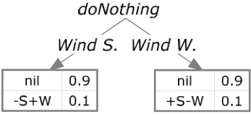
IRRESPECTIVE OF THE AGENT’S ACTION. ... 47 FIGURE 2.5:STATE TRANSITION DIAGRAM FOR THE COIN FLIPPING AGENT WITH AN ADDITIONAL WIND SPEED
FEATURE.THE PROBABILITIES FOR THE “DO NOTHING” ACTION ARE SHOWN.FLIP ACTION PROBABILITIES ARE OMITTED. ... 48 FIGURE 2.6:INFLUENCE DIAGRAM REPRESENTING A FACTORED STATE MODEL FOR A COIN FLIPPING AGENT. 49 FIGURE 2.7:STRUCTURED CPT REPRESENTATION OF CONDITIONAL PROBABILITY TABLES FOR INFLUENCE
DIAGRAMS. ... 49 FIGURE 2.8:PSO REPRESENTATION OF THE FLIP ACTION. ... 52 FIGURE 2.9:PSO REPRESENTATION OF THE DONOTHING ACTION... 52 FIGURE 3.1:A LATTICE SHOWING FREQUENT ITEM-SETS WITH ASSOCIATED OCCURRENCES IN A TRANSACTION
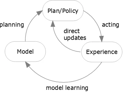
DATABASE.THE OCCURRENCE COUNT OF COMBINED ITEM-SETS IN THE LOWER LEVELS OF THE LATTICE CANNOT BE HIGHER THAN THE MINIMUM OCCURRENCES OF A PARENT ITEM-SET. ... 65 FIGURE 4.1:INTEGRATED PLANNING, ACTING AND LEARNING. ... 73 FIGURE 4.2:BATCHMODELQ.THE PROCESS SEPARATES MODEL LEARNING AND POLICY FORMATION
(PLANNING) STAGES.THE POLICY CAN BE USED TO SELECT ACTIONS IN RESPONSE TO PERCEPTS RECEIVED FROM THE ENVIRONMENT. ... 76 FIGURE 5.1:THE “SLIPPERY GRIPPER” ENVIRONMENT.THE ROBOT’S TASK IS TO PAINT BLOCKS WHICH ARRIVE
11
FIGURE 5.4:UPDATE TO OPERATORS IN THE “SLIPPERY GRIPPER” DOMAIN WITH ADDITIONAL DEPENDENCIES BETWEEN OUTCOMES (THE GRIPPER ALWAYS BECOMES WET IF THE BLOCK IS PAINTED). ... 90 FIGURE 6.1:SUBSET OF THE LEVEL 2 RULE ELEMENT SETS RELATED TO THE DRYER ACTION IN THE “SLIPPERY
GRIPPER” DOMAIN ... 121 FIGURE 7.1:THE “SLIPPERY GRIPPER” ENVIRONMENT. ... 139 FIGURE 7.2:BACKGROUND KNOWLEDGE FOR THE “SLIPPERY GRIPPER” ENVIRONMENT WITH ADDITIONAL
“CLEAN” PERCEPTUAL FEATURE. ... 141 FIGURE 7.3:THE P-SPO SET FOR A “SLIPPERY GRIPPER” ENVIRONMENT WITH EXACTLY ONE BLOCK AND ONE
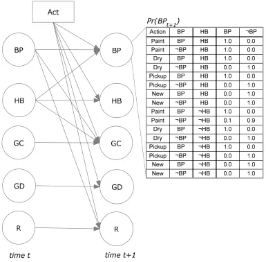
GRIPPER. ... 143 FIGURE 7.4:INFLUENCE DIAGRAM SHOWING DEPENDENCIES BETWEEN VARIABLES FOR THE “SLIPPERY
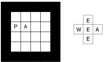
GRIPPER” ENVIRONMENT.THE CONDITIONAL PROBABILITY (CPT) TABLE FOR THE BP VARIABLE HAS BEEN INCLUDED.OTHER CPTS (OMITTED FOR BREVITY) WOULD FOLLOW A SIMILAR FORMAT. ... 144 FIGURE 7.5: PREDATOR AND PREY IN A 4×4 GRID (P= PREDATOR AGENT;A= PREY AGENT).THE SENSOR
INFORMATION FOR THE PREDATOR,P, IS SHOWN TO THE RIGHT (W= WALL.E= EMPTY,A= PREY AGENT). ... 146 FIGURE 8.1:GRAPH OF ERROR MEASURE OF GENERATED STATES GENERATED FROM MODELS GENERATED
FROM DATA COLLECTED OVER 100,1000,5000,10000,20000,50000 AND 100000 RANDOM MOVES. ... 153 FIGURE 8.2:GRAPH OF TIME TAKEN (IN SECONDS) TO LEARN A P-SPO SET OR TABULAR MODEL WITH DATA
COLLECTED FROM 100,1000,5000,10000,20000,50000 AND 100000 RANDOM MOVES. .... 156 FIGURE 8.3:GRAPH OF REWARD GATHERED AFTER FOLLOWING A POLICY DERIVED FROM A MODEL LEARNED
FROM DATA COLLECTED FROM 100,1000,5000,10000,20000,50000 AND 100000 RANDOM MOVES. ... 157 FIGURE 8.4:P-SPOS GENERATED BY ASDD WITH A TRAINING DATA SET OF 100,000 FOR THE “SLIPPERY
GRIPPER” DOMAIN. ... 159 FIGURE 8.5:GRAPH OF ERROR MEASURE OF GENERATED STATES GENERATED FROM MODELS GENERATED
FROM DATA COLLECTED OVER 100,1000,5000,10000,20000,50000 AND 100000 RANDOM MOVES. ... 162 FIGURE 8.6:GRAPH OF TIME TAKEN (IN SECONDS) TO LEARN A P-SPO SET OR TABULAR MODEL WITH DATA
COLLECTED FROM 100,1000,5000,10000,20000,50000 AND 100000 RANDOM MOVES. .... 163 FIGURE 8.7:GRAPH OF REWARD GATHERED AFTER FOLLOWING A POLICY DERIVED FROM A MODEL LEARNED
12
FIGURE 8.8:MATCHING P-SPOS FOR THE MOVE(SOUTH) ACTION IN THE PREDATOR-PREY ENVIRONMENT FOR A SET OF OPERATORS ACQUIRED FROM 50,000PDIS EXPERIENCES. ... 166 FIGURE 10.1:GRAPH OF REWARD GATHERED AFTER FOLLOWING A POLICY DERIVED FROM A MODEL LEARNED
FROM DATA COLLECTED FROM 100,1000,5000,10000,20000,50000 AND 100000 RANDOM MOVES. ... 191 FIGURE 10.2:NEW OPERATOR VALUES AFTER 10,000 ITERATIONS OF RVRL WITH AGGREGATION BY AVERAGE
FUNCTION FOR RULES LEARNED USING ASDD FROM 100,000PDIS IN THE SLIPPERY GRIPPER
ENVIRONMENT... 192 FIGURE 10.3:NEW OPERATOR VALUES AFTER 10,000 ITERATIONS OF RVRL WITH AGGREGATION BY
VARIANCE FUNCTION FOR RULES LEARNED USING ASDD FROM 100,000PDIS IN THE SLIPPERY GRIPPER ENVIRONMENT... 192 FIGURE 10.4:P-SPO SET FOR THE DRYER ACTION WITH VARIANCE WEIGHTED RULE VALUES FOR AN OPERATOR SET LEARNED FROM 20,000PDIS. ... 194 FIGURE 10.5:P-SPO SET FOR THE PICKUP ACTION WITH VARIANCE WEIGHTED RULE VALUES FOR AN
OPERATOR SET LEARNED FROM 20,000PDIS. ... 195 FIGURE 10.6:P-SPO SET FOR THE DRYER ACTION WITH VARIANCE WEIGHTED RULE VALUES FOR AN OPERATOR SET LEARNED FROM 20,000PDIS. ... 195 FIGURE 10.7:P-SPO SET FOR THE PICKUP ACTION WITH VARIANCE WEIGHTED RULE VALUES FOR AN
OPERATOR SET LEARNED FROM 20,000PDIS. ... 196 FIGURE 10.8:GRAPH OF REWARD GATHERED AFTER FLOWING A POLICY DERIVED FROM A MODEL LEARNED
13
List of Tables
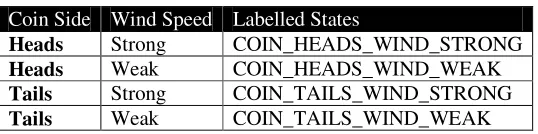
TABLE 2-1:A TABULAR WORLD MODEL BUILT BY LABELLING STATES USING EMPIRICAL EVIDENCE ... 46 TABLE 2-2:COIN SIDE AND WIND SPEED ARE FEATURES IN A FACTORED STATE MODEL.THE STATE OF THE
WORLD CAN BE DESCRIBED BY THE STATES OF EACH OF THE FEATURES THAT DESCRIBE IT, OR BY A LABEL DEFINING THE COMBINED STATES. ... 46 TABLE 3-1:BUILDING A TABULAR WORLD MODEL BY LABELLING STATES USING EMPIRICAL EVIDENCE ... 58 TABLE 6-1:A SAMPLE OF PERCEPTUAL DATA ITEMS FOR THE “SLIPPERY GRIPPER” BLOCK PAINTING AGENT. 110 TABLE 8-1:ERROR MEASURE OF GENERATED STATES GENERATED FROM RULES LEARNED FROM DATA
COLLECTED OVER 100,1000,5000,10000,20000,50000 AND 100000 RANDOM MOVES. ... 153 TABLE 8-2: MISSING STATES VS. EXTRA STATES GENERATED BY EACH MODEL.THE FIRST NUMBER IN EACH
CELL IS THE NUMBER OF STATES MISSING FROM THE MODEL AND THE SECOND NUMBER INDICATES EXTRA STATES GENERATED BY THE MODEL. ... 155 TABLE 8-3: TIME TAKEN (IN SECONDS) TO LEARN A P-SPO SET OR TABULAR MODEL WITH DATA COLLECTED
FROM 100,1000,5000,10000,20000,50000 AND 100000 RANDOM MOVES. ... 156 TABLE 8-4: REWARD GATHERED AFTER FOLLOWING A POLICY DERIVED FROM A MODEL LEARNED FROM DATA
COLLECTED FROM 100,1000,5000,10000,20000,50000 AND 100000 RANDOM MOVES. .... 157 TABLE 8-5: GOALS ACHIEVED VS. DISASTER STATES ENCOUNTERED AFTER FOLLOWING A POLICY DERIVED
FROM A MODEL LEARNED FROM DATA COLLECTED FROM 100,1000,5000,10000,20000,50000 AND 100000 RANDOM MOVES.THE FIRST NUMBER IN EACH CELL IS GOALS ACHIEVED.THE SECOND NUMBER IS DISASTER STATES ENCOUNTERED. ... 158 TABLE 8-6:ERROR MEASURE OF GENERATED STATES GENERATED FROM RULES LEARNED FROM DATA
COLLECTED OVER 100,1000,5000,10000,20000,50000 AND 100000 RANDOM MOVES. ... 161 TABLE 8-7: MISSING STATES VS. EXTRA STATES GENERATED BY EACH MODEL.THE FIRST NUMBER IN EACH
CELL IS THE NUMBER OF STATES MISSING FROM THE MODEL AND THE SECOND NUMBER INDICATES EXTRA STATES GENERATED BY THE MODEL. ... 162 TABLE 8-8: TIME TAKEN (IN SECONDS) TO LEARN A P-SPO SET OR TABULAR MODEL WITH DATA COLLECTED
FROM 100,1000,5000,10000,20000,50000 AND 100000 RANDOM MOVES. ... 163 TABLE 8-9: REWARD GATHERED AFTER FOLLOWING A POLICY DERIVED FROM A MODEL LEARNED FROM DATA
COLLECTED FROM 100,1000,5000,10000,20000,50000 AND 100000 RANDOM MOVES. .... 164 TABLE 10-1: REWARD GATHERED AFTER FOLLOWING A POLICY DERIVED FROM A MODEL LEARNED FROM
14
TABLE 10-2: REWARD GATHERED AFTER FOLLOWING A POLICY DERIVED FROM A MODEL LEARNED FROM DATA COLLECTED FROM 100,1000,5000,10000,20000,50000 AND 100000 RANDOM MOVES. ... 197
15
List of Algorithms
ALGORITHM 2-1: DIRECTENVIRONMENTUPDATE.S= STATE,A= AGENT,E= ENVIRONMENT DEFINITION ... 37 ALGORITHM 2-2: ENVIRONMENT.S= STATE,A= AGENT,E= ENVIRONMENT DEFINITION. ... 40 ALGORITHM 2-3: BODYENVIRONMENTUPDATE.S= ENVIRONMENT,A= AGENT,E= ENVIRONMENT
DEFINITION. ... 40 ALGORITHM 3-1:MULTI-STREAM DEPENDENCY DETECTION (MSDD).D= SET OF PERPETUAL DATA ITEMS, F
= AN EVALUATION FUNCTION, MAXNODES = THE MAXIMUM NODES THAT CAN BE EXPLORED. ... 61 ALGORITHM 3-2: FILTER(R).R= COMPLETE SET OF CANDIDATE RULE ELEMENT SETS. ... 63 ALGORITHM 4-1:THE DYNA-Q ALGORITHM FOR DETERMINISTIC ENVIRONMENTS (ADAPTED FROM [87]).
MODEL(S,A) DENOTES THE CONTENTS OF THE MODEL.THE STEPS BEFORE THE MODEL(S,A) STEP IMPLEMENT STANDARD TABULAR Q-LEARNING.THE REMAINING STEPS IMPLEMENT MODEL BASED LEARNING. ... 75 ALGORITHM 4-2: BATCHMODELQ-MODELENVIRONMENT.THE ALGORITHM REPEATEDLY TAKES RANDOM
ACTIONS IN AN ENVIRONMENT TO BUILD UP A DATABASE OF PERCEPTUAL DATA ITEMS (PDIS).PDIS ARE USED TO LEARN A MODEL VIA A BATCH LEARNING ALGORITHM. ... 77 ALGORITHM 4-3: BATCHMODELQ-FORMSAMPLEPOLICY.M= THE ENVIRONMENT MODEL, P = AN INITIAL
PERCEPT, A = AN INITIAL ACTION.THE ALGORITHM USES REINFORCEMENT LEARNING TO UPDATE VALUES IN THE MODEL FROM SAMPLE SUCCESSOR PERCEPTS AND REWARDS. ... 78 ALGORITHM 4-4: BATCHMODELQ-FORMDISTRIBUTIONPOLICY.M= THE ENVIRONMENT MODEL, P = AN
INITIAL PERCEPT, A = AN INITIAL ACTION.THE ALGORITHM USES DYNAMIC PROGRAMMING TO UPDATE STATE-ACTION VALUES IN THE MODEL FROM THE SET OF SUCCESSOR PERCEPTS AND REWARDS. ... 79 ALGORITHM 4-5: BATCHMODELBELLMAN-FORMDISTRIBUTIONPOLICY.M= THE ENVIRONMENT MODEL, P =
AN INITIAL PERCEPT.THE ALGORITHM USES BELLMAN UPDATES TO UPDATE STATE VALUES IN THE MODEL. ... 79
ALGORITHM 4-6: GREEDYACTION.M= THE ENVIRONMENT MODEL WITH ASSOCIATED VALUES, P = AN INITIAL PERCEPT.THE ALGORITHM RETURNS THE HIGHEST VALUED ACTION AVAILABLE FOR THE PERCEPT. ... 80 ALGORITHM 5-1: GENERATESAMPLEPERCEPT.P= INITIAL PERCEPT,A= ACTION,PSPOS =P-SPO SET.A
SAMPLE PERCEPT IS RETURNED. ... 93 ALGORITHM 5-2: GENERATEPERCEPTSANDPROBS.P= PERCEPT,A= ACTION,PSPOS = PLANNING OPERATOR
16
ALGORITHM 6-2: SUBSET.C= CANDIDATE RULE ELEMENT SETS.PDI= PERCEPTUAL DATA ITEM. ... 118 ALGORITHM 6-3: APRIORIGEN.LK-1= CANDIDATES AT LEVEL K-1 ... 118 ALGORITHM 6-4: JOIN.L= RULE ELEMENT SETS AT PREVIOUS LEVEL. ... 120 ALGORITHM 6-5: APRIORIPRUNE.CK = CANDIDATES AT LEVEL K.LK-1= RULE ELEMENT SETS AT LEVEL K. . 120 ALGORITHM 6-6: APRIORIFILTER.CK = CANDIDATES AT LEVEL K,LK-3= CANDIDATES AT LEVEL K-3, GLEVEL =
G-STATISTIC LEVEL FOR SIGNIFICANCE TESTS. ... 123 ALGORITHM 6-7: EXTRACTONERULEELEMENTSETS.D=DATABASE OF PERCEPTUAL DATA ITEMS. ... 125 ALGORITHM 6-8: ADDRULECOMPLEMENTS.R= COMPLETE RULE SET.D= DATABASE OF PERCEPTUAL DATA
ITEMS. ... 126 ALGORITHM 6-9: CREATEPSPOS.R= COMPLETE RULE SET.A= SET OF POSSIBLE AGENT ACTIONS.THE
ALGORITHM RETURNS P, A SET OF P-SPOS BUILD FROM THE RULE SET. ... 128 ALGORITHM 6-10: PRECEDENCE.PSPOS=THE OPERATOR SET.D= PERCEPTUAL DATA ITEMS.THE ALGORITHM SETS THE PRECEDENCE BETWEEN ALL OPERATORS.PRECEDENCE DEFINES WHICH OPERATOR WILL BE USED IF THERE IS A CONFLICT. ... 130 ALGORITHM 6-11: MATCHING.PSPO= THE PLANNING OPERATOR SET.PDI= A SINGLE PERCEPTUAL DATA
ITEM.THE ALGORITHM RETURNS THE SUBSET OF PLANNING OPERATORS WITH CONTEXT AND ACTION MATCHING THE PDI. ... 130 ALGORITHM 6-12: FIRSTPSPOSUPERIOR.PSPO1 AND PSPO2= THE PLANNING OPERATORS TO BE TESTED.D
= THE SET OF PERCEPTUAL DATA ITEMS.THE ALGORITHM RETURN TRUE IF THE FIRST P-SPO WILL HAVE PRECEDENCE IN SITUATIONS WHERE THE RULES ARE IN CONFLICT. ... 131 ALGORITHM 6-13: APRIORIPRUNE.MODIFIED FOR THE ASDDS OPTIMISATION FOR ASDD. ... 137 ALGORITHM 8-1: FINDMODELERROR.M=MODEL TO BE COMPARED.THE FUNCTION RETURNS THE ERROR
MEASURE FOR THE MODEL TO BE COMPARED AGAINST AN EXHAUSTIVE TABULAR MODEL FOR THE SAME ENVIRONMENT... 152 ALGORITHM 9-1:RVRLUPDATE(PSPOS, P, A). P = PERCEPT, A = ACTION. ... 177 ALGORITHM 9-2: RULEVALUEITERATION.PSPOS=THE PLANNING OPERATOR SET, P=INITIAL PERCEPT,
A=INITIAL ACTION.THE ALGORITHM TAKES A SET OF P-SPOS AND ITERATIVELY IMPROVES THE UTILITY ESTIMATE ASSOCIATED WITH EACH OPERATOR FOR N-STEPS. ... 179 ALGORITHM 9-3: BESTACTION.PSPOS=THE PLANNING OPERATOR SET, P=INITIAL PERCEPT.THE ALGORITHM
RETURNS THE BEST ACTION FOR THE GIVEN PERCEPT. ... 180 ALGORITHM 9-4: VARIANCE RULEVALUEITERATION.PSPOS=THE PLANNING OPERATOR SET, P=INITIAL
17
ALGORITHM 11-1:G STATISTIC. D1= GENERAL RULE, D2= SPECIFIC RULE, SC IS THE SUPPORT COUNT FOR THE RULE IN THE OBSERVED DATA, BS IS THE SUPPORT COUNT FOR THE BODY (CONDITIONS) OF THE RULE IN THE OBSERVED DATA.THE ALGORITHM RETURNS THE G STATISTIC MEASURE OF NON-INDEPENDENCE BETWEEN D1 AND D2. ... 224 ALGORITHM 11-2: APPLYBYSAMPLE(P,PSPO).P= INITIAL PERCEPT,PSPO= THE P-SPO TO APPLY.THE
ALGORITHM RETURNS A SINGLE PERCEPT WITH ONE OF THE OUTCOMES OF THE P-SPO APPLIED USING PROBABILISTIC SAMPLING. ... 225 ALGORITHM 11-3: APPLYALLOUTCOMES(P,PSPO,PROB).P= INPUT PERCEPT.PSPO=P-SPO TO APPLY.
PROB = PROBABILITY ASSOCIATED WITH INITIAL PERCEPTS.THE FUNCTION APPLIES THE OUTCOMES OF EACH OF THE OUTCOME-SETS OF THE P-SPO IN TURN TO THE PERCEPT, AND RETURNS A SET OF
18 ACHNOWLEDGEMENTS:
I’d like to thank my tutor, Dr. Kostas Stathis, for helping me to find both a fascinating research area and a range of techniques to explore within it. Our meetings have been exactly as academic research should be: inspiring, motivating and resulting in the phrase “needs further research”. I have also been fortunate in having a second tutor Dr. Artur Garcez who provided the motivation to help me finish the thesis, guidance on analysis techniques, and the understanding that the life of a part-time student requires a subtle mix of carrot and stick. I’d also like to thank Dr. Andrew Tuson for introducing me to City University and helping to further my career as an academic. Thank you to all the staff of the School of Informatics at City University for your continued support and assistance.
19
Declaration
I hereby declare that:
• my submission as a whole is not substantially the same as any that I have previously
made or am currently making, whether in published or unpublished form, for a
degree, diploma, or similar qualification at any university or similar institution
• the following parts of the work or works now submitted have previously been
submitted for a qualification at a university or similar institution (only brief details
required):
. . .
. . .
. . .
• until the outcome of the current application to this University is known, the work or
works submitted will not be submitted for any qualification at another university or
similar institution.
Date: . . . Signature: . . .
21 ABSTRACT:
This thesis presents an approximate dynamic programming (ADP) technique for environment modelling agents. The agent learns a set of parallel stochastic planning operators (P-SPOs) by evaluating changes in its environment in response to actions, using an association rule mining approach. An approximate policy is then derived by iteratively improving state value aggregation estimates attached to the operators using the P-SPOs as a model in a Dyna-Q-like architecture. Reinforcement learning and dynamic programming are powerful techniques for automated agent decision making in stochastic environments. Dynamic programming is effective when there is a known environment model, while reinforcement learning is effective when a model is not available. The techniques derive a policy: a mapping from each environment state to an action which optimizes the long term reward the agent receives.
The standard methods become less effective as the state space for the environment increases because they require values to be associated with each state, the storage and processing of which is exponential to the number of state variables. Resolving this “curse of dimensionality” is an important topic of research amongst all communities working on this problem. Two key methods are to: (i) derive an estimate of the value (approximate dynamic programming) using function approximation or state aggregation; or (ii) build a model of the environment from experience. This thesis presents a method of combining these approaches by exploiting structure in the state transition and value functions captured in a set of planning operators which are learnt through experience in the environment. Standard planning operators define the deterministic changes that occur in an environment in response to an action. This work presents Parallel Stochastic Planning Operators (P-SPOs), a novel form of planning operator providing a structured model of the state transition function in environments which are both non-deterministic and for which changes can occur outside the influence of actions. Next, an automated method for extracting P-SPOs from observations in an environment is explored using an adaptation of association rule mining. Finally, methods of relating the state transition structure encapsulated in the P-SPOs to state values, using the operators to store state value aggregation estimates, are evaluated.
The framework described provides a method by which approximate dynamic programming can be applied by designers of AI agents and AI planning systems for which they have minimal prior knowledge. The framework and P-SPO based implementations are tested against standard techniques in two bench-mark stochastic environments: a “slippery gripper” block painting robot; and a “predator-prey” agent environment.
23
1.
Introduction
It has been the aim of many AI researchers to create an autonomous agent that can be situated
in an environment and learn to act effectively through discovery of the mechanics of the
world they inhabit. This has been termed “developmental AI” [40] or “constructivist AI”
[28][84] and is discussed as early as 1950 in Turing’s paper “Computing, Machinery &
Intelligence” [92] in which the idea of building a simulation of an infant’s mind that could be
trained through interaction with the world was proposed as one method of constructing a
machine that could pass, what later became known as, the Turing test.
Turing’s motivation for this aim was a practical one of solving issues with adaptability. It was
clear that an artificial intelligence could not be programmed to respond to every eventuality
that it could encounter, and that even if this knowledge could be given, it would soon become
out of date as the environment changed. Some mechanism was therefore needed to adapt to
the changing conditions and the development of knowledge by discovery promised an
approach that required minimal programmer effort if appropriately general principles could be
discovered.
This adaptability motivation is reflected in a number of agent-based applications, and is
particularly apparent in the fields of adversarial AI and non-player character AI (NPC AI) in
computer game applications. Computer games are played by humans, who continually adapt
their strategies to improve their performance. If a weakness is found in an adversarial AI’s
behaviour, then the game will quickly become uninteresting if the AI opponent keeps
re-playing the same losing strategy. A developmental approach could help the AI adapt to these
changing strategies. NPC’s in computer games can be adversaries (e.g. bots in FPS games), in
which case the same argument applies, but they can also be helpers to the main character (e.g.
a war-horse in a role-playing game), or simply background characters aimed at improving the
aesthetics of the environment (e.g. a villager in a town the character travels through). Each of
these agent types could benefit from a developmental approach that allows a designer to
specify the type of behaviour that is required without having to specify the means of
achieving it.
In this context an autonomous agent is considered to be a decision-making entity. It is situated
in some environment or world, and has a number of actions that it can carry out. It has a
method of perceiving its environment, and makes decisions as to which of the available
actions it will select. It is autonomous in the sense that it can actively perform action selection
24
from the environment into a percept, and uses information contained within these percepts to
guide its actions through some form of deliberation [49].
The type of agent studied in this research builds a model of its world by evaluating changes to
the received percepts over time, and models the effects of its available actions by evaluating
the changes in perception in response to the actions selected. The agent is given a reward
mechanism, which indicates a preference that the agent should have for perceiving that it is in
a particular state. The agent then uses its model to make decisions by forming a plan or
policy. A plan is a deterministic set of actions, which lead the agent from its current state to a
reward state. In stochastic (random) environments the agent cannot establish a deterministic
set of actions and must, instead, create a strategy which takes into account every state it could
find itself in. This strategy is called a policy (or universal plan), and is a mapping from every
possible state to an action.
Planning in a stochastic environment in which actions have probabilistic outcomes, the
environment changes outside the agent’s control, or the agent has uncertain knowledge about
the environment state, presents unique challenges which are not present in classical planning
systems, such as STRIPS [31] or the situation calculus [57]. The random nature of the
environment, from the agent’s perspective, means it needs a mechanism for selecting action in
situations or which are unexpected, or which it may not have encountered before. For large
environments an exact definition of such a plan becomes impossible and approximation
techniques are required. Such techniques fall under the categories of approximate dynamic
programming (ADP) [73] and Decision Theoretic Planning [7].
The work presented here investigates the creation of an agent which:
• Builds a planning operator based model of its world through interaction. Planning
operators describe the expected changes to the environment in response to the agent’s
actions.
• Uses the model, to attach utility estimates (estimates of expected future rewards) to
the planning operators.
• Uses the utility estimates to provide a policy. The agent can select an action to
activate the operators with the highest utility estimate. Given an initial percept, the
agent can make a decision by finding the highest valued action available for that
25
The syntax of the planning operators acquired by the agent will be covered in depth in
chapter 5. In order to introduce the concept, a simple example of an operator set for an agent
is given below.
The agent has two actions: flip or doNothing in an environment consisting of a single coin
which can be showing either heads or tails. It receives a reward of 1.0 if the coin is showing
heads and 0.0 otherwise:
{
}
{
}
0.5 : ( , )
( ) :{} (0.5)
0.5 : ( , )
: ( , ) 1.0 : ( , ) (1.0)
: ( , ) 1.0 : ( , ) (0.0)
showing coin heads
flip coin U
showing coin tails
doNothing showing coin heads showing coin heads U
doNothing showing coin tails showing coin tails U
→
→
→
Each operator has:
• An action: e.g. flip(coin).
• A context: e.g. showing(coin, heads).
• An outcome set with associated probabilities. e.g. {0.5:showing(coin, heads),
0.5:showing(coin, tails)}
• A utility: e.g. U(0.5).
The outcome set identifies the expected changes to the environment in response to the action
if the context holds. The utility is an estimate of the expected future rewards if the action is
taken in the given context. The task in this case is episodic (has terminating states). The
episode length is one, with both showing(coin, heads) and showing(coin, tails) being
terminating stares. This means that only immediate rewards affect the utility.
The agent can form a policy by selecting the action with the best available utility in the given
context. If, for example, the coin is currently showing heads, then the flip action can be taken
(because it has no context) or the doNothing action can be taken (with showing(coin, heads)
context). These have utilities of 0.5 and 1.0 respectively, and an agent attempting to maximise
reward gather would, therefore, select the doNothing action, resulting in an immediate reward.
A method of learning operators of this type, along with their more complex parallel
extensions, is defined in chapter 6, and evaluated in chapter 8. Methods of attaching utility
estimates to planning operators are investigated in chapter 9, and evaluated in chapter 10.
Empirical learning of planning operators in stochastic environments is challenging because:
• An action may have uncertain effects inherently (e.g. the result of a “flip” action on a
26
• The effects of an action may be masked by external elements (e.g. multiple coins are
flipped simultaneously by others and the agent wrongly attributes the result of their
others actions to its own).
• The action conditions may be masked by external elements (e.g. the state of the coin
the agent flips may randomly match the state of one of the other coins before the flip
action, and the agent incorrectly concludes that the state of the other coin is an
important condition for the flip action).
Each of these issues can be tackled, to some extent, by performing statistical significance
testing, and the planning operator learning mechanism presented in chapter 6 is based on this
technique.
Standard dynamic programming techniques can build a utility map of a state space by cycling
through each state, taking the best available action (according to the current estimate, or a
random action in order to explore) and, when a reward is encountered in the following state,
feeding this reward back to the previous state. The number or values which must be calculated
is, however, exponential to the number of features present in the state space. This is referred
to as the “curse of dimensionality” [73]. Attaching utilities to the operators removes the need
for storage of these values, but poses a new set of challenges:
• Each planning operator’s conditions represent only a small proportion of all the
possible conditions of each state. The utility estimate attached to the operator is
therefore an aggregation of many states from the full state-space.
• Planning operators are applied in parallel to calculate the following state. The agent
therefore needs a mechanism for deciding the contribution made by each operator to
the utility of taking a particular action.
• Total utility in a reinforcement learning system increases (or decreases) as the
learning progresses. Operators with fewer conditions will increase (or decrease) in
utility as a consequence of being applied more regularly, while those with more
conditions will learn more slowly.
The general framework of utility-based action-selection is provided by dynamic programming
(for model-based approaches), and reinforcement learning (for model-free approaches) [87].
The approach used in this research is initially model-free, learning the model from experience
and can therefore be seen as fitting into both fields. The utilities learned by the agent provide
estimates of the utility of being in a particular state and the approach therefore fits into the
27
A range of model-based learning techniques have been proposed for agent-based planning
mechanisms. The work presented here builds on contributions from several sources:
• Model based reinforcement learning: Dyna-Q [88].
• Planning operator learning: multi-stream dependency detection [64], noisy deictic
rules [67] and association rule mining [1].
• Factored state mode approaches for decision theoretic planning [10].
• Approximate Dynamic Programming [73].
1.1
Motivation
The hypothesis of this thesis is that utility estimates attached to acquired parallel stochastic
planning operators, describing the dynamics of a predictably probabilistic environment, can
be used to compactly model the effectiveness of taking actions in that environment.
The general motivation for the work is to create agents that are both autonomous learners and
who’s behaviour is comprehensible by human designers. The drive comes largely from the
author’s commercial background in computer game agent programming. Games companies
are generally reticent to use black-box techniques (such as a neural network), despite their
obvious ability to deliver complex AI with reduced designer input, because a bug found in a
solution requires a complete re-train. This newly re-trained solution can itself contain errors,
and the risks are perceived as too great when it is considered that the error may only be
discovered a week away from shipping a title with a multi-million dollar budget [12].
The use of rule-based models allows designers to either re-write rules by hand or,
alternatively, interpret the errors by investigation and make adjustments to parameters or
learning conditions when generating new rules.
Attaching values to rules means that the policy itself can be interpreted by designers, because
they can see which actions and rules are favoured by the system in certain situations.
The particular properties of many computer game agent environments that make this
technology applicable are that:
• An accurate model of the dynamics of the environment, from the perspective of an
individual agent, is not known in advance, and often cannot be created due to the
stochastic nature of the environment or the unpredictable actions of agents within it.
• Experience can be gathered through trial runs with negligible cost, as opposed to the
28
Some of the properties of the system that provide an advantage as a computer game agent
controller include:
• Intelligible rules: the system creates rules that can be read and understood by a human
designer.
• The rules can be modified by hand if necessary.
• The system can generalise over unseen states and therefore produce intelligent
behaviour based on knowledge gained in similar situations.
• Limited processing power is required at run-time, with the learning occurring off-line.
• The design of AI agent controllers for computer games is an expensive process, often
requiring highly skilled and experienced developers with extensive domain
knowledge of each game. Automating this process could lead to significant cost
savings and improvements in computer games.
1.2
Aims & Objectives
Techniques exist for creating effective agent controllers which exhibit some of the properties
outlined above, but not all. The overall aim is to produce an effective and practical technology
that inherits aspects of the best of these systems and exhibits each of the above desirable
properties.
• Create a framework for environment modelling agents: the framework should be
adaptable, in that a variety of environment modelling systems and action selection
mechanisms can be incorporated.
• Design a rule-based environment modelling system: the system should have the
expressive power to model the environment from the point of view of the agent. It
must, therefore be able to model events that happen outside the agents control
(environment actions), unpredictable/stochastic action outcomes, outcomes that are
both independent and non-independent, and combinations of these. The rule system
also needs to be in a human readable form and preferably in a form familiar to AI
researchers in order to enable “glass-box” interpretation.
• Design a system for learning the rule-based environment modelling system from
experience: human designers are not adept at creating probabilistic rule systems by
hand. The environment modelling system should be able to acquire a model by
29
operators by discovering patterns in changes to the environment in response to actions
(or when no action is taken).
• Design a system for attaching utility estimates to the rules: allowing compact storage
and human interpretable values to be attached to rules. The system should have the
capacity to build rule utility estimates from successor rule utility estimates, without
the need to enumerate the value of every state, or state-action pair in the environment.
1.3
Framework
The framework for the agent’s learning consists of the following elements:
1) Embodiment: the agent is embodied, and situated in an environment: it can select
actions (behaviours) available through its body and receives percepts, which are a
function of the current environment state.
2) Modelling: the agent builds a model of its perception of the environment using
parallel stochastic planning operators (P-SPOs). These are learnt empirically by
observing the effects of actions through percepts. The percepts before and after each
action are used as training data for a P-SPO learning algorithm. Note that the
environment itself may be deterministic, but viewed through the agent’s percepts, can
appear stochastic.
3) Policy generation: the agent builds a policy by simulating actions using the
environment model encapsulated in the rules. In initial tests, the agent uses standard
dynamic programming to build a policy from simulated experience extracted from the
model. In the full system, value estimates are attached to each operator. The operators
contain actions and are therefore acting as a set of aggregation estimates
encapsulating information in the form: taking action, a, under conditions, c, has
utility, u.
A useful property of the framework is that the policy generation phase is entirely simulated
and can therefore be seen as “free” in terms of cost to the agent in the environment.
Additionally, the agent’s goals can be changed, but the rules describing the environment’s
dynamics remain unchanged. It can therefore be set new tasks or goal without the need to
re-model the environment [90].
1.4
Contributions
30
• A framework for developmental AI is created: a world model learning phase is
followed by a planning phase using approximate dynamic programming. Extensions
for in-line learning are explored.
• Parallel Stochastic Planning Operators (P-SPOs) are defined: an extension of Noisy
Deictic Rules [67] to include provision for independent outcomes.
• Apriori Stochastic Dependency Detection (ASDD) is defined & evaluated: a fast
stochastic rule learning algorithm for construction of P-SPOs from observation data
using statistical significance and data mining methods.
• Rule Value Reinforcement Learning (RVRL) is defined & evaluated: a state
aggregation method for approximate dynamic programming, using P-SPOs as
aggregation estimates for a state aggregation function.
Experimentation is performed to evaluate:
• The performance of P-SPOs as an environment model for a dynamic programming
based policy generator.
• The performance of RVRL in generating policies for agent action.
1.5
Structure
Chapters 2 and 3 provide background for environment modelling techniques from the
perspective of agents, and methods of planning (policy formation) using the model. Chapter 4
provides the overall model-based learning framework used in the research. Chapter 5 defines
parallel stochastic planning operators (P-SPOs). Chapter 6 defines the ASDD algorithm and
associated functions for learning P-SPOs from data. Chapter 7 defines the test environments
used in this research. Chapter 8 provides the results of the ASDD rule learning algorithm in
terms of environment modelling and policy generation using a standard dynamic
programming algorithm. Chapter 9 then defines the RVRL algorithm for attaching rule values
to operators. Chapter 10 shows the results of the complete system, with values attached to
operators learned in the framework and used as a policy. Chapter 11 discusses the
achievements of the system, related work and future improvements to the system.
1.6
Previous Publications
The framework presented in chapter 4 and evaluation technique (chapter 8) have previously
31
technique for planning operator learning in "SMART (Stochastic Model Acquisition with
ReinforcemenT) Learning Agents: A Preliminary Report." [17].
The ASDD method for learning stochastic logic rules (chapter 6) was defined and evaluated
in "The Apriori Stochastic Dependency Detection (ASDD) Algorithm for Learning Stochastic
Logic Rules." [18].
Rule Value Reinforcement Learning (RVRL) for attaching values to planning operators
(chapter 9) was first presented in "Rule Value Reinforcement Learning for Cognitive Agents"
[16] and further evaluation in the context of an embodied agent environment modelling
framework was published in “Learning to Act with RVRL Agents" [15]. Peer review
comments from this and extensions to widen the applicability of the system have been
incorporated in the approximate dynamic programming based update functions for RVRL
33
2.
Background I: Agents, Environments & Models
This chapter introduces the agent and environment definitions which underpin this work.
Embodied agents, with environment interaction mediated through action selection in an agent
body, are defined and presented in the context of both deterministic and stochastic
environments. Techniques for representing an environment model from the perspective of an
agent are presented. The model representations are chosen because they define the evolution
of the environment in response to agent action (allowing planning) and can be can be acquired
from data.
2.1
Agents
The purpose of the system presented in this work is to create effective controllers for
autonomous agents. A broad definition of an agent, as given by Wooldridge [98], is:
“An agent is a computer system that is situated in some environment, and that is capable of
autonomous action in this environment in order to meet its design objectives”.
This definition puts no requirements on the agent to be part of a multi-agent system, to be able
to communicate, or any of the other uses for which agents are employed. It simply defines an
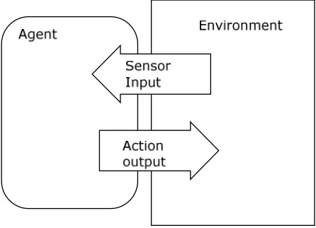
[image:34.612.192.415.407.568.2]agent as a decision maker, situated in an environment.
Figure 2.1: An agent and its environment. The agent produces actions in response to sensory
input.
Figure 2.1 shows that the agent responds to sensor input from the environment with actions.
This definition is broad in that there is no requirement for the agent to respond with intelligent
decisions, and the type of environment is not defined. The agent is situated in an environment,
34
If the agent is treated as a separate decision making entity, outside the environment, then
flexible agent architectures can be produced (as investigated by the EU SOCS project [85]). A
good analogy is to consider a human playing a computer game. The human has a view of the
world and can select actions through the controller, but these actions do not directly change
the environment. Instead, they are stored as the next action that will be taken by the player
when the game-world updates. The human player can easily be replaced by an artificial
intelligence. If we give the AI a view of the world and allow it to trigger the same actions,
then it should require no further change to the game world to integrate the AI. This view of
embodiment is explored further in section 2.1.4.
The following section gives an abstract definition of agents and environments. The term agent
is, in general, somewhat loosely defined and has been used in the definition of complex
environments and interactions. Rather than debate these points, the intention here is to
provide a useful definition of agency based around an embodied “perceive, deliberate,
execute” framework, which will enable definitions from dynamic programming to be set in an
agent context.
2.1.1 Agent: Action Selection within an Environment
A useful starting point for defining agents and environments is given by Wooldridge [98]. An
environment is assumed to have a set of possible world states S, where S = {s1, s2, s3, …, sn}.
At any given time the environment can be in one of these states. Environments can have an
infinite or a discrete number of states. An agent has a set of actions, A, which can influence
this state, where A = {a1, a2, a3, …, an}.
The agent’s purpose is to choose an action (make a decision). An agent can be viewed as a
function, mapping a history of environment states, S*, to an action.
* :
action S →A (2.1)
A reactive agent is an agent with no memory, which can only take account of the current state
of the environment when deciding upon its next action. It is, therefore, defined by the
function:
:
action S→A (2.2)
A deterministic environment can be modelled as a function mapping the current state of the
environment and the agent’s action to a new state:
:
35
Starting from a state s∈S, the execution of the environment function on an action a∈A
produces a new state. A non-deterministic environment can be modelled as a mapping from
state and action to a set of next states:
: ( )
env S× →A
ϑ
S (2.4)This model appears simple but succinctly defines the agent as being a decision making entity,
separate from its environment, but able to influence the environment. The environment
function can be as complex as is required, containing multiple agents or just one single agent.
This abstract definition is simple and can be used to describe almost any agent, but it does not
help in the practical construction of an agent.
Wooldridge provides a next step, which is to add perception to the agent, which captures the
agent’s ability to sense its environment, and that this sensing is an incomplete representation
of the environment state. The see function takes a state and outputs a percept, where P = {p1,
p2, p3, …, pn}.
:
see S→P (2.5)
The action function is then altered to become a function of the history of percepts for a
cognitive agent, or a single percept for a reactive agent:
* :
action P →A (2.6)
Note that the mapping from states to percepts is generally not one-to-one. The number of
possible percepts is less than or equal to the number of possible states, with several different
states may mapping to the same percept. From the agent’s perspective, two states that map to
the same percept are indistinguishable. If each state maps to exactly one percept, then the
environment is said to be fully observable.
The agent architecture employed in this work uses this form, with the additional layer of
separation provided by the agent body, which is part of the environment and is the agent’s
only method of interaction with the environment (see section 2.1.4).
2.1.2 Agent: Perceive, Deliberate and Execute
A second perspective on the basic agent architecture is given by Ferber [30]. The definition,
again, separates the agent’s decision making process from the environment, but is more
explicit in including multiple agents making simultaneous decisions in the environment. The
agent is considered as three functions:
36
• Deliberate
• Execute.
The perceive function is defined separately for each the agent in the system. It associates a
percept with each state of the world and can be defined as a mapping from the state of the
environment to a set of available percepts for an agent. An agent, g, has a perceive function
defined as:
g g
perceive : S→P (2.7)
The deliberate function for a reactive agent is equivalent to that defined by Wooldridge. It
takes a history of percepts and produces an action. Reactive agents have no memory or state
and therefore the deliberate function consists simply of a reaction, modelled here by mapping
a percept directly to action:
:
g g
deliberate P →A (2.8)
Cognitive agents have the ability to retain information, and thus act on the basis of
perceptions and past experiences. Their deliberation process is therefore divided into memory
and decision functions. The agent’s capacity for memory can be characterised by an internal
state sg∈Sg (the set of internal states of agent g). Memorising an experience is defined as
moving from one internal state to another. The memorisation function takes an internal state
and a perceptand produces a new internal state:
:
g g g g
mem P ×S →S (2.9)
The deliberate function of a cognitive agent takes a percept and an internal state and produces
an action to perform:
:
g g g g
deliberate P ×S →A (2.10)
The “execute” function in Ferber’s definition, takes an individual agent’s action and the
current environment state and produces a set of influences, which will be combined by the
environment function to transform the world’s state.
: g g
execute A × → ΓS (2.11)
These influences are intended to resolve issues with ordering of execution in the agent
environment. If execution order is not an issue, then the execute function can be adapted to
directly transform the environment state:
: g g
37
The environment function (action of the environment) can be represented as a special type of
agent producing influences:
:
:
E
e E
environment S A
execute S A →
× → Γ (2.13)
If execution order is not an issue, then the environment function can be mapped as a direct
translation from state to state:
:
environment S→S (2.14)
2.1.3 Environment Update Function: Direct Action, Discrete Time
An environment update function using the direct execution of actions for multiple agents
(adapted from [30]) is presented below. The algorithm updates the state by processing the
action of all agents in the environment, and then updates the state using the environment
function. The environment function in this case could be replaced by a function executee, but
keeping the function explicit will aid explanation in the following sections.
for all (a A) {
p = perceive (S);
a = deliberate (p);
S = execute (S,a);
}
S = environment(S,E);
a a a
∈
directEnvironmentUpdate(S,A,E)
Algorithm 2-1: directEnvironmentUpdate. S = state, A = agent, E = environment definition
A variation on this algorithm forms the update function at the core of almost all current
computer games (see [59] and [38] for examples). Computer games use discrete time updates
so that a predictable performance occurs each time the algorithms are executed (avoiding
differences due to precision errors). These discrete time-steps can be set to varying amounts
for different aspects of the update, such that the agent’s decision process may execute in 100
millisecond steps, while fast moving objects are simulated every 10 milliseconds.
For computer game simulations, the agent decision making processes is required to be
flexible, such that a human could take the place of the agent as decision maker, with minimal
code changes. This can be achieved using the embodied agent concept (below), in that the
agent’s execute function has the effect of changing the agent’s body state, so that a new action
38
2.1.4 Embodied agents
The concept of an agent body is often useful in drawing the boundary between agent and
environment in both robot control [11] and reinforcement learning. Sutton and Barto make the
following observation [87]:
“In particular, the boundary between agent and environment is not often the
same as the physical boundary of a robot’s or animal’s body. Usually, the
boundary is drawn closer to the agent than that. For example the motors and
mechanical linkages of a robot and its sensing hardware should usually be
considered parts of the environment rather than parts of the agent…
Anything which cannot be changed arbitrarily by the agent is considered to
be outside of it and thus part of the environment.”
The agent perceives the world through the sensors of this body and acts in the world by
triggering actions (behaviours) in the body. The agent itself is therefore detached from the
environment in two ways:
• The agent’s actions do not have a direct effect on the environment: the effects of an
agent body on the environment mediate them.
• The agent’s perception of its environment is not a complete picture of the
environment: it is a reflection of the state of that environment as filtered through the
agent body’s sensors.
Embodied agents make explicit the distinction between the agent, its interface with the
environment, and the environment itself. The agent’s only means of gaining input from the
environment is through sensors, which the environment updates. The perceive function maps
these sensors to a percept. The agent’s only means of output to the environment is by
selecting actions. The selected action is stored in the body state. These actions are then
executed by the agent body through its update function. The agent body is, in this respect, no
39
Figure 2.2: Embodied agents. The agent is a separate decision making entity whose contact
with the environment is mitigated through an agent body. The agent selects the next action to
be executed by the body and receives input by converting sensor information into percepts.
Sensors gather information from the environment (including the agent’s body).
The agent itself can be thought of as the mind of the body. If the required interface exists
between the agent and its body, the mind could be considered to be operating outside the
environment. The environment can proceed without intervention from the agent, with the
environment acting as an external control mechanism. The agent body would, of course, be
inactive without the agent’s selection of actions, but its state can still be changed by the
environment.
At a high level, the logical representation of the agent is unchanged from that presented in
section 2.1.1, because the agent’s body is part of the environment, and therefore remains part
of the environment function. It is now possible, however, to be more explicit in modelling the
environment as a set of objects with state, and the agent body as a special object with a set of
available actions and a sensing mechanism.
The environment function below takes as input the current state, S, the set of agents, A, and
40
o
E
a
for all (o S) {
S = update (S);
}
S = update (S);
for all (a A) {
a.body.sensors sense (S);
}
∈
∈
= environment(S,A,E)
Algorithm 2-2: environment. S = state, A = agent, E = environment definition.
The environment (including the agent body) is modelled as a set of objects, which are updated
each time the environment updates. If the environment updates by a uniform amount each
time, this is referred to as a discrete time environment.
:
: o
E update S S
update S S →
→ (2.15)
Initially, all objects update the state of the environment. Next, the environment function
updates all objects. Finally, all agent sensors are updated by mapping the current state of all
environment objects (including the agent body) to the sensors using each agent’s sense
function.
The body based update function can now be defined. The update for all agents is altered to
reflect the fact that the agent can only update its percept based on the contents of its sensors,
and can only influence the environment through the changes to its body state. The execution
of actions is no longer part of the agent, and is instead part of the environment update function
(defined above). The individual agent’s action changes the agent’s body state by selecting
actions.
a a
a
for all (a A) {
p = perceive (a.body.sensors);
a = deliberate (p);
a.body.state = execute (a.body.state,a);
}
S = environment(S,A,E); ∈
bodyEnvironmentUpdate(S,A,E)
Algorithm 2-3: bodyEnvironmentUpdate. S = environment, A = agent, E = environment
41
The agent uses it’s perceive function to receive a percept from the sensors and sends a choice
of action to the agent body each time the environment is updated. The effects of the agent’s
actions are mediated through the agent body and its interactions with other objects in the
environment.
Note that this is an approximate architecture, aimed at showing the interface between the
agent and its body. Simulated environments such as those used in computer games can add
multiple levels of complexity to incorporate factors such as collision detection, event
propagation and network capabilities. The aim here is to provide the simplest environment
definition which demonstrates the separation between the agent and its environment, while
being flexible enough to incorporate more complex architectures.
This distinction between agent body and environment is broadly similar to that defined by the
PROSOCS agent template [86]. The architecture is flexible in that it can be applied equally to
agents embodied in robots, virtual agents (e.g. NPCs) in computer game environments
embodied in avatars, or to any system in which a view and controller separates the agent from
its environment.
Although more sophisticated formal definitions of agency exist, these are mainly geared
toward refinements for individual agent types. The representation used is complete for the
purposes of this research and is compatible with that used by Markov models which form a
key element of the framework presented in chapter 4.
2.2
Environment Model
The term environment model is used to describe a function which can provide simulated
experience of an environment. For a fully observable deterministic environment, this is a
function mapping states and actions to successor states.
An environment model, from the perspective of an agent, can refer to any system that the
agent can use to predict the outcome of its actions. Given an input state, s, and action, a, a
model gives a prediction of the successor state, s’. For a deterministic environment this will
take the same form as a sample model:
: '
sampleModel s a× →s (2.16)
If the environment is stochastic (random) then each state and action can lead to a set of
possible next states, S’, with each member of the set having an associated probability, Pr. A
distribution model is a model that produces all possible successor states and associated