A Variational Approach to Problems in Calibration of Multiple Cameras.

City, University of London Institutional Repository

Citation

:

This is the accepted version of the paper.

This version of the publication may differ from the final published

version.

Permanent repository link: http://openaccess.city.ac.uk/4709/

Link to published version

:

Copyright and reuse:

City Research Online aims to make research

outputs of City, University of London available to a wider audience.

Copyright and Moral Rights remain with the author(s) and/or copyright

holders. URLs from City Research Online may be freely distributed and

linked to.

City Research Online: http://openaccess.city.ac.uk/ [email protected]

A Variational Approach to Problems in Calibration

of Multiple Cameras

Gozde Unal

, Anthony Yezzi

, Stefano Soatto

, and Greg Slabaugh

Abstract

This paper addresses the problem of calibrating camera parameters using variational methods. One problem addressed is the severe lens distortion in low cost cameras. For many computer vision algorithms aiming at reconstructing reliable representations of 3D scenes, the camera distortion effects will lead to inaccurate 3D reconstructions and geometrical measurements if not accounted for. A second problem is the color calibration problem caused by variations in camera responses that result in different color measurements and affects the algorithms that depend on these measurements. We also address the extrinsic camera calibration that estimates relative poses and orientations of multiple cameras in the system, and the intrinsic camera calibration that estimates focal lengths and the skew parameters of the cameras. To address these calibration problems, we present multi-view stereo techniques based on variational methods that utilize partial and ordinary differential equations. Our approach can also be considered as a coordinated refinement of camera calibration parameters. To reduce computational complexity of such algorithms, we utilize prior knowledge on the calibration object, making a piecewise smooth surface assumption, and evolve the pose, orientation, and scale parameters of such a 3D model object without requiring a 2D feature extraction from camera views. We derive the evolution equations for the distortion coefficients, the color calibration parameters, the extrinsic and intrinsic parameters of the cameras, and present experimental results.

Index Terms

calibration, variational methods, color calibration, lens distortion calibration, camera parameters refinement.

1

Siemens Corporate Research, Princeton NJ 08540. Corresponding author: [email protected]

2

School of Electrical Engineering, Georgia Institute of Technology, Atlanta GA 30332.

3

I. INTRODUCTION

The problem of recovering a 3D representation of a scene from multiple 2D images has been one

of the main research interests in computer vision. Many of the existing stereo techniques involve

pre-processing the camera images to extract 2D features such as corners, lines, and contours of objects in the

scene. These features are then used to find correspondences between camera views. In practice, searching

for features and establishing correspondences is not an easy task due to noise and local extrema. Early

variational approaches to the 3D reconstruction problem were pioneered by Faugeras et.al. [1] who also

relied on local feature matching. A more recent variational approach by Yezzi and Soatto [2, 3] proposed

a joint region-based image segmentation and simultaneous 3D stereo reconstruction technique. This paper

addresses camera calibration techniques built on this later stereo reconstruction framework that avoids

searches for local correspondences and is versatile enough to accommodate the new applications to be

shown. A tradeoff is achieved by making a piecewise smooth object assumption and a constant background

assumption, however, extraction of 2D features from given camera views are not required.

Camera calibration refers to the problem of finding the mapping between the 3D world and the camera or

image plane. For most computer vision algorithms aimed at reconstructing reliable digital representations

of 3D scenes, accurate camera calibrations are essential. There has been a great deal of research on

camera calibration problem as early as in 70’s [4]. In most of the previous techniques, some set of

features are extracted from images of a known calibration pattern, and intrinsic camera parameters as

well as camera pose and orientation (extrinsic camera parameters) are estimated by a minimization of an

overall cost functional [5–13]. Many calibration techniques use both nonlinear minimization and closed

form solutions as in [14].

In this paper, we develop a coordinated refinement technique for the extrinsic camera parameters,

calibration parameters in a coupled way within a multiple camera system1_{. For geometrical measurements,}

an intrinsic camera parameter, the camera lens distortion, is an important issue, and will result in inaccurate

3D reconstructions if not taken into account. Another common problem in multi-view stereo techniques

is caused by color miscalibrations between cameras due to different sensor characteristics. Extrinsic

parameters of the cameras on the other hand, determine the relative poses and orientations of cameras,

and their correct estimation is one of the first phases of a camera calibration system.

A. Relation to Previous Work and Contributions

1) Lens Distortion: The ideal pinhole camera model leads to imaging of world lines as lines on the

image plane, and simplifies many computations and considerations [6]. However, for most real cameras

with wide-angle or inexpensive lenses this assumption does not hold, and nonlinearities introduced by a

well-known phenomenon referred to as a lens distortion should be taken into account. The corresponding

distortion parameters should be estimated for each camera.

In many existing calibration techniques, good estimates for extrinsic and intrinsic camera parameters

are first obtained by a pinhole camera model neglecting lens distortion. Then distortion calibration is

performed while holding the other parameters fixed [17–19]. This is possible because the mapping from

3D world coordinates to the 2D image plane can be decomposed into a perspective projection and a

mapping that models the deviations from the ideal pinhole camera.

A popular group of lens distortion calibration methods in the literature, mainly under the category known

as plumb line methods, rely on a first step of extracting edges from the images. Either a user manually

selects the image curves or there must be a way to reliably estimate image edges which correspond to

linear 3D segments in the world. An optimization problem is set up by defining a measure of how much

each detected segment is distorted. The curved lines in the image which do not really correspond to 3D

line segments will constitute outliers in this optimization procedure [17, 20–23]. Other techniques such

1

An initial version of this work that addresses lens distortion and color calibration can be found in [15] and [16], and an initial work

as [24] rely on point correspondences. Given a set of 3D points, the associated epipolar and trilinear

constraints are arranged into a tensor, which is computed with estimated distortion parameters at each

step to minimize a reprojection error in an iterative manner. In another group of methods as in [25–27], a

direct solution strategy is employed to find camera calibration parameters by incorporating lens distortion

as well.

Our contribution is a new distortion calibration technique that does not rely on extraction of edges and

search for point correspondences. The former may not be an easy task due to noise and local extrema.

Instead, we devise an integrated calibration technique in which the distortion parameters of cameras are

computed in a tightly coupled framework. The desired coupling of multiple camera views comes from

estimating a common 3D object (in this case the calibration object). In other words, we minimize the

cost between the reprojection of the 3D calibration object and the image measurements by evolving the

distortion parameters of the cameras. In our distortion calibration algorithm, we use a white bar object,

made from a foam core as shown in Fig.1 on the left. We capture its views before a dark background

with the multi-view stereo rig system, a desktop multi-camera system designed for remote multimedia

collaboration, developed by HP Labs [28]. The images of the calibration object captured from three of

the five cameras in the rig are given in Fig.1. Many desktop multi-camera systems use wide angle and

inexpensive cameras which produce severe distortion effects as can be observed in the given images.

Fig. 1. Three out of five camera views of the real calibration object shown on the left.

As we will show, with this technique we can also incorporate other parameters of calibration into the

same variational framework and get their locally optimal estimates as well.

2) Color Calibration: Another common problem in multi-view stereo techniques is caused by color

characteristics, ambient conditions like temperature, manufacturing differences, and so on. These yield

dif-ferent color measurements between cameras, and affect the algorithms that depend on these measurements.

Camera color calibration refers to the problem of estimating the color calibration parameters of cameras

to overcome these unwanted effects. A common approach taken toward this problem is to calibrate each

camera independently through comparisons with known colors on a color calibration object/environment

[28, 29].

The color calibration object we use, shown in Fig.2 is a color cube with patches of known colors whose

Fig. 2. Photograph of the color calibration object.

images are captured from each camera. Demosaicing coefficients are calculated independently for each

camera based upon the absolute colors of the calibration object and the measured color responses of each

camera. Slight errors and differences that arise from this independent calibration procedure sometimes

lead to noticeable seams or discontinuities in the texture mapping process during the transition of the

texture map between neighboring cameras. Our goal is to help even out these discrepancies by devising

a relative inter-camera color calibration technique in which the demosaicing parameters of cameras are

calculated jointly in a tightly coupled framework rather than just one camera at a time.

Similar to our approach to lens distortion calibration, the desired coupling of the multiple camera

views comes from estimating a common 3D shape, and in addition a common radiance function for the

calibration object (in this case, the color cube). We take advantage of the fact that the object shape is

known up to location and scale to simplify the problem. Hence, we estimate the pose parameters of the

cube, the radiance function on the cube, and the color calibration coefficients for each camera.

3) Extrinsic and Intrinsic Calibration: Following the same philosophy as mentioned in the other two

calibration problems above, extrinsic and intrinsic calibration parameters can be estimated in a variational

It should be noted that due to differential nature of the estimation equations derived, the extrinsic

and intrinsic update equations require rough initial values. This is a well-known feature of almost all of

the recent state-of-the-art energy functionals used in segmentation (e.g., Mumford-Shah energy, geodesic

energy, ...), i.e., the solutions are locally optimal, hence starting far away from the real solution may lead

to solutions that get stuck at local extrema far from the desired solution. Nevertheless, the usefulness of

a refinement stage in extrinsic and intrinsic camera parameters will be demonstrated via the improvement

in the final 3D reconstructions. A nice feature of the methodology presented in this paper is that it can

integrate several different problems in geometric and color calibration into an overall unified system based

on the joint segmentation framework to evolve pose, color, distortion, extrinsics, and intrinsics.

The organization of this paper is as follows. We first present a variant of the Yezzi-Soatto algorithm

in which a 3D object is allowed to move with a semi-affine motion model in Section II. We developed

this scheme for our applications in calibration, where the 3D object shape is roughly known (up to 3

scales and rigidity) to obtain more efficient and faster algorithms. We then present a novel technique for

lens distortion calibration in Section III and a novel technique for relative inter-camera color calibration

in Section IV. We apply the same calibration ideas for intrinsic camera calibration in Section V, and for

extrinsic camera calibration problem in Section VI. Conclusions and discussions are given in Section VII.

II. EVOLUTIONEQUATIONS OF3D OBJECTMOTIONPARAMETERS

The Yezzi-Soatto 3D stereo reconstruction model builds a cost on the discrepancy between the

reprojec-tion of a model surface with a radiance f :R3 −→R, the background (infinitely far away) with radiance

b :_R3 _−→

R, and the actual measurements from multiple camera views. Let gi denote the transformation

from world coordinates to camera coordinates:gi :X−→Xi = (Xi, Yi, Zi)T, andπdenote the perspective

transformation from camera frame to the image plane: π :X_{i −→}x_{i = (xi =} Xi

Zi, yi =

Yi

Zi)

T_.

On the image plane, the cost functional for the Yezzi-Soatto model can be written as a joint segmentation

and with 3 color channels k ∈(R, G, B):

E = X

k=R,G,B n

X

i=1

Z

Ri

[fk((π◦gi)−1(xi))−Iik(xi)]2dΩi+

X

k=R,G,B n

X

i=1

Z

Rc i

[bk−Iik]2dΩi (1)

This energy can be lifted back onto surface S :

E(S) = X

k=R,G,B n

X

i=1

Z

S

[(fk_(X)−Ik

i(π◦gi(X)))2−(bk−Iik) 2_{] X}

i(X)σ(Xi)dA, (2)

where σ is the Jacobian of the change of coordinates from the image plane to the surface, Xi is the

visibility function of a voxel on the surface, and dA is the area measure of surfaceS. The deformation of

the surface S w.r.t. this energy or data fidelity measure is then obtained by finding the partial differential

equation (PDE) that is the gradient descent flow of the energy E. A popular class of numerical techniques

known as Level Sets Methods [30], is utilized to evolve the surface S via the evolution of a 3D function

Ψ : R3 −→ R. Nevertheless, an update of the level set function is required after each iteration of the

associated PDE, and even with more efficient narrowband schemes [31], there is a considerable amount

of computation involved. For our intended applications, in which there is a calibration object whose shape

can be roughly known a priori, rather than deforming the surface of the 3D object, we will evolve its pose

and scale parameters instead. Next, using the energy E in Eq. 2 we will derive the ordinary differential

equations (ODEs) to update the parameters of the surface motion modeled by a semi-affine transformation,

which is more general than a similarity but less general than a fully affine transformation.

Let the original rigid surface be denoted by So, thenS =gs(So), orX=gs(Xo) =RsXo+Ts, and let

λ denote parameters of the rigid motion gs _{of the surface S}

o with rotation Rs and translation Ts. Then

the gradient of the energy E w.r.t. λ is given by:

∂E(λ) ∂λ =

X

k=R,G,B

Z

S

X

i

Fk i (X)<

∂X

∂λ,N> dA+ ∂Fk

i (X)

∂λ dA

= X

k=R,G,B

Z

So

X

i

Fk

i (gs(Xo))<

∂(gs_X o)

∂λ ,RsNo > dAo

+ 2(fk_(gX

o)−Iik)<

∂(gs_X o)

∂λ ,∇f

k

where Fk

i = [(fk(X)−Iik(π◦gi(X)))2−(bk−Iik)2] Xi(X)σ(Xi)is the Mumford-Shah term from Eq. 2

(also in [2]). The derivation follows from shape optimization tools [32] that provide the shape derivatives

in curve and surface evolution framework. N _{denotes the surface normal vector. Note that the visibility}

functionXi(gs(Xo)), included in the data termFik(·)is computed using the original visibility function but

compensated by RT

s(Ci−Ts)), whereCi is a camera center. The second term in Eq.(3) is the region term

corresponding to the foreground object whereas the first one is the boundary term. In our applications,

the background is modeled by a piecewise constant radiance, therefore we omit the background region

term in the equation.

For translation parameters:

< ∂(g

s_X o)

∂λ ,RsNo >=RsNo.

For rotation parameters:

<∂(g

s_X o)

∂λ ,RsNo>=<Rs



      

0 Zo −Yo

−Zo 0 Xo

Yo −Xo 0



      

| {z }

ˆ

X_o

,RsNo>=<−RsXˆo,RsNo>, (4)

where we utilize exponential coordinates (see [33] for details on this representation) for the global rotation

parameters of the surface. We note that a matrix in an inner product expression, when operated on a vector,

will incorporate each of its row vectors in the inner product to result in a vector: <x1,x2, ...,xn,y>= (<

x1,y>, <x2,y>, ..., <x_n,y>).

For further flexibility in initializing a model surface, we add three scaling parameters along the X, Y,

and Z axes. Then the semi-affine transformation for a point X_{o on the surface becomes:} X _=gs₍X_{o) =}

RSX_o+T_{, where} S=



      

sx 0 0

0 sy 0

0 0 sz



      

. The gradient of the energy w.r.t. the scaling parameters λ=sj is

derived similarly to the above:

X

k=R,G,B

Z

So

X

i

Fik(g s

(X_o))< ∂(g

s_X o)

where

<∂(g

s_X o)

∂λ ,RsNo> = <Rs ∂S

∂λXo,RsNo> with e.g. ∂(gs_X

o)

∂s1

= Rs

∂S ∂s1

Xo=Rs

       

1 0 0

0 0 0

0 0 0        

Xo=Rs

       

Xo.x

0 0        

<∂(g

s_X o)

∂λ ,RsNo> = <Rs

                Xo 0 0                 0 Yo 0                 0 0 Zo                

| {z }

RX

s

, RsNo> . (5)

The evolutions for the rigid motion parameters λ are then given by the gradient descent equations:

∂λ ∂t =−

∂E ∂λ =−

X k=R,G,B Z So X i

Fik(g s

(X_o))

| {z }

Fk

R_sN_{o dAo, (for translation). (6)}

∂λ ∂t =−

∂E ∂λ =−

X

k=R,G,B

Z

So

Fk _<−R

sXˆo,RsNo > dAo, (for rotation). (7)

∂λ ∂t =−

∂E ∂λ =−

X

k=R,G,B

Z

So

Fk <RX_{s ,}R_sN_{o > dAo, (for scaling). (8)}

Here note that the visibility function Xi(gs(Xo)) is computed using the original visibility function but

compensated by the S−1RT

s(Ci−Ts) ), where S−1=

       

1/sx 0 0

0 1/sy 0

0 0 1/sz

       

. Note that we can generalize

this idea in a straightforward fashion by considering S _{to be more general than a simple diagonal matrix}

in order to accommodate a fully affine motion of the surface.

We will use equations (6-7-8) in updating the pose of the surface S to estimate its correct placement

III. LENS DISTORTION CALIBRATION

The lens distortion is usually modeled by a function defined from the ideal image plane to the distorted

image plane. One approach is to decompose it into two terms: radial and tangential distortion [17]. The

radial distortion is a deformation along the radial direction from a center of distortion point to an image

point, and the tangential distortion is a deformation in a direction perpendicular to the radial direction,

and is negligible for many cameras. To model the radial distortion effects, a commonly used distortion

function D(r) is given by (1 +k1r2+k2r4+...) where r is the radius from the center of distortion to a

point on the ideal image plane. The principal point (u0, v0) is often used as the center for radial distortion

[6], which we will also adopt. Below xˆ_{i is the distorted image coordinates, and D is the distort function:}

ˆ

x_{i =D}x_{i = (1 +k}i

1r2+k i

2r4+...)xi, (9)

r2 _{= (x}2

i +yi2), and kji is the jth distortion coefficient for camera i. In Eq. 9, we assume that k0 = 1,

which can be changed to an arbitrary k0 value.

A. Calibration of the Lens Distortion Parameters

Notation: World X−→

|{z}

gi

Xi−→

|{z}

π xi=

0 B B B B B

Xi

Zi =xi

Yi

Zi =yi

1

1 C C C C C A

−→

|{z}

Lu 0 u0

0 Lv v0

0 0 1

(u, v) (image coordinates), where D is the

distort function in Eq. 9, and Lu and Lv are the focal lengths. The gradient of the energy (1), assuming

a single image channel over the distorted image plane, w.r.t. distortion parameters ki

j is given by

∂ki j

∂t =− ∂E ∂ki j

=−

Z

ˆ ci

Fi((D◦π◦gi)−1xˆi)<

∂xˆ_i ∂ki j

,nˆ_{i > dˆs (10)}

where Fi = (f−Ii)2−(b−Ii)2, subscript icorresponds to each camera view, and nˆi denotes the normal

vector to the occluding boundary cˆi of region Ri on the distorted image plane. We only consider the

boundary term (sˆ is the arclength of the contour cˆi on the image plane: the distorted or actual image

coordinates) as we assume the foreground and background have constant radiance. We design the lens

We want to lift this integral back onto occluding boundary Ci of the surface. Note that ∂ˆ_∂kxi_j are given

by

∂xˆ_i ∂ki 1

=r2x_i, ∂xˆi

∂ki 2

=r4x_{i, ...} ∂xˆi

∂ki j

=r2jx_i

hence

< ∂ˆxi ∂ki j

,nˆ_{i > dˆs=< r}2j_π(X_{i), J} ∂

∂s(D◦π)Xi > ds=< r

2j_π(X

i), JD′◦π′

∂

∂sXi > ds (11)

where J denotes the 2×2 ninety degree rotation matrix, D′ _{= (1 +k}

1r2 +k2r4+...), and

π′ = 1 Z2 i    

Zi 0 −Xi

0 Zi −Yi



 

 (12)

is the Jacobian of the perspective projection π. We can continue to simplify:

<∂xˆi ∂ki j

,nˆi> dsˆ=r2jD′<[π(Xi)]2×1,

1 Z2 i     0 1

−1 0        

Zi 0 −Xi

0 Zi −Yi

    _∂X i ∂s

3×1

> ds = r 2_j D′ Z2 i <     Xi Yi     1 Zi ,    

0 Zi −Yi

−Zi 0 Xi

    _∂X i ∂s

3×1

> ds

= r

2j_D′

Z3 i <        

0 −Zi

Zi 0

−Yi Xi

            Xi Yi    ,

∂Xi

∂s > ds= r2j_D′

Z3 i <        

−ZiYi

ZiXi

0        

,∂Xi ∂s > ds

Noting that        

−ZiYi

ZiXi

0        

=Xi×

        Xi Yi 0        

, we have < ∂xˆ_i

∂kj,nˆi> dˆs=

r2j_D′ Z3

i <−

        Xi Yi 0        

×Xi,∂

X_i

∂s > ds, and

< ∂xˆi ∂ki j

,nˆ_{i > dˆs=−}r

2j_D′

Z3 i

<X_i× ∂Xi

∂s ,        Xi Yi 0       

> ds=−r

2j_D′

Z3 i

<||X_i||N_i,

       Xi Yi 0       

> ds. (13)

Substituting Eq.(13) into Eq.(10), we get the calibration equation

∂ki j ∂t = Z Ci Fi

r2_j

D′

||Xi||

Z3 i

<N_i,

        Xi Yi 0        

for the lens distortion parameters ki

j. Note that the distortion calibration method we propose can handle

different models of distortion by changing the D function, and related derivatives in Eq.(14).

B. Using Several Poses of the Object

When camera views from multiple poses of the object are available, we can take advantage of the

existence of variously distorted views in calibrating the lens distortion. In the first phase, we estimate

both pose and distortion coefficients from separate experiments. To simplify the explanation, let us assume

that we want to solve for only one distortion coefficient ki

1 for each camera i. Once we obtain rough

estimates for the object pose and distortion coefficients ki

1, we can fuse a “common distortion” ˜k1i from

these separate experiments for each camera i and then jointly evolve k˜i

1’s as follows:

∂˜ki 1

∂t =

Mposes

X

m=1

Z

Ci,m

Fi,m

r2_j

D′

||X_i,m||

Z3 i,m

<Ni,m,



      

Xi,m

Yi,m

0 

      

> ds. (15)

At the same time, we evolve the pose parameters of separate poses of the object as described in Section II,

the only difference being the incorporation of the new “common distortion” in the equations. For instance,

we evolve any of them for a given pose as follows:

∂λ ∂t =−

X

i

Z

So

Fi(gs(Xo))<

∂(gs_X o)

∂λ ,RsNo> dAo (16)

where Fi includes computation of Ii(D·π·gi (gs(Xo)))with the new common distortion coefficients k˜1i

in the multiplying distortion factor D.

C. Experimental Results

For our calibration algorithm, we initialize a surface model of the real calibration object which is shown

from several vantage points in Fig.3. After initializing the surface, the first phase of our algorithm is to

evolve its pose parameters to position the 3D object model roughly in the correct location in 3D space.

For the experiments presented here captured via HP Labs’ stereo rig system, we used three different poses

of the pose parameters are shown in Fig.4, for three different pose captures of the calibration object in

each column (showing only one camera view for each pose). The distortion coefficients are also evolved

at a slower pace. That is, the time step used in the associated ODE is small in the first phase. In the

experiments, the distortion function D in (9) with one distortion coefficient k1 for each camera is used.

After the separate evolutions for each of the poses have converged, common initial distortion coefficients

are computed as the average of the results from phase 1. In the second phase of the algorithm, we evolve

the distortion coefficients for each camera again separately but summed over different poses. We show

sample views of pose 1, 2, and 3 in row 1 of Fig.s 5-6-7. As the distortion coefficients converge to true

values, the reprojection of the surfaces onto the distorted views results in a better match to the image data

and continues to minimize the overall energy. Such images with reprojections are shown on the second

row of Figures 5-6-7. The undistorted views shown as well on the third row. The straightening effect of

this operation on the curved lines can be clearly observed in these images.

IV. COLORCALIBRATION

For color calibration, the differences in absolute colors measured in the response of each camera are

modeled by a simple multiplicative factor in each of color RGB channel measurements and an additive

offset parameter.

The first variation of our energy functional E using this model leads to gradient descent flows:

∂E ∂αi,k

=−

Z

Ri

[fk_−(α

i,kIik+βi,k)]IikdΩi−

Z

Rc i

[bk_−(α

i,kIik+βi,k)]IikdΩi, (17)

∂E ∂βi,k

=−

Z

Ri

[fk_−(α

i,kIik+βi,k)]dΩi−

Z

Rc i

[bk_−(α

i,kIik+βi,k)]dΩi. (18)

for the color calibration parameters αi,k and βi,k for each camera i, and k ∈ {R, G, B}, where Iik, fk,

and bk _{are from one of the three color channels {R, G, B}. Note that one can extend this framework to}

RGGB images in a straightforward fashion.

In our test calibration experiments, we utilized white noise additive offsets and multiplicative scaling

a synthetically created example in Fig.8, where the correct geometry and radiance function are known,

we show such miscalibration effects on the original views, and views during the evolution of αi’s and

βi’s in Eq.s (17-18), and views after these parameters have converged. In addition, in Fig.9, the curves

depict the true α andβ values for all nine camera views, and the convergence of the estimated parameters

towards the real values.

Similarly in Figure 10, the color cube with original colors are shown from some camera views first,

then shown after their color calibration parameters are perturbed. Finally, the convergence of the color

parameters results in a corrected set of colors as shown in the views. Also shown in Figure 11 are the

evolutions of the color calibration parameters for the shown views. We have to note here again that due to

relative calibration framework among cameras, the updated parameters may not always result in absolute

values but still provide useful outputs for the multi-camera systems.

V. INTRINSIC PARAMETER CALIBRATION

We show the evolution of three of the main intrinsic camera parameters: focal lengths, denoted by Lu

and Lv for each of the coordinates on the image plane, and the skew parameter a. Inclusion of the skew

parameter between the two plane coordinates leads to an intrinsics matrix of the form

π=



     

Lu a u0

0 Lv v0

0 0 1



     

,

then the Jacobian of the perspective transformation becomes (compare to Eq. 12):

π′ ₌



  

Lu/Zi a/Zi −LuXi/Zi2−aYi/Zi2

0 Lv/Zi −LvYi/Zi2



  =

1 Z2

i



  

LuZi aZi −LuXi−aYi

0 LvZi −LvYi



  .

The derivatives of the image coordinates w.r.t. each of the intrinsic parameters are computed from the

overall energy functional as before (similar to our derivations of the lens distortion calibration parameters

in Section III):

∂E ∂Lj

= X

k=R,G,B

Z

Ci

[(fk_−Ik i)

2_−(bk_−Ik i)

2_]

| {z }

Fk

∂xi

∂Lj

For the focal length parameter Lu, we have

< ∂xi ∂Lu

,ni> ds =

∂πCi

∂Lu , ∂ ∂sJπ ′ Ci ds = * ∂ ∂Lu    

LuXi/Zi+aYi/Zi

0    , 1 Zi 2    

0 LvZi −LvYi

−LuZi −aZi LuXi+aYi



  

∂Xi

∂s + ds (19) = 1 Z3 i *        

0 −LuZi

LvZi −aZi

−LvYi LuXi+aYi

            Xi 0    ,

∂Xi

∂s > ds=

1

Z3 i

< Lv

        0

ZiXi

−YiXi

       

,∂Xi ∂s + ds. Noting that         0

ZiXi

−YiXi

       

=Xi×

        Xi 0 0        

, then for the focal length parameter Lu we obtain:

< ∂xi ∂Lu

,ni> ds =

1

Z3 i

<−Lv

        Xi 0 0        

×Xi,

∂Xi

∂s > ds

= −Lv

Z3 i

<Xi×

∂Xi

∂s ,         Xi 0 0        

> ds=−Lv||Xi||

Z3 i

<Ni,

        Xi 0 0        

> ds. (20)

Due to the skew parameter, the equations for the second focal length parameterLv will be slightly different.

This time incorporating the derivative w.r.t. Lv in Eq. 19 :

< ∂xi ∂Lv

,ni> ds=

1 Z3 i <        

0 −LuZi

LvZi −aZi

−LvYi LuXi+aYi

            0 Yi    ,

∂Xi

∂s > ds=

1 Z3 i <        

−LuZiYi

−aZiYi

LuXiYi+aYi2

       

,∂Xi ∂s > ds

Again noting that

       

−LuYiZi

−aZiYi

LuXiYi+aYi2

       

=Xi×

       

−aYi

LuYi

0        

, then for the focal length parameter Lv, we have:

< ∂xi ∂Lv

,n_{i > ds=−}||Xi||

Z3 i

<N_i,

      

−aYi

LuYi

0       

Note that when the skew parameter a is 0, which is a widely used convention, the above equation reduces

to a symmetric form of the Eq. 20 derived for Lu.

Finally, we derive similarly the update equations for the skew parameter a:

<∂xi

∂a,ni> ds=

1 Z3 i <        

0 −LuZi

LvZi −aZi

−LvYi LuXi+aYi

            Yi 0    ,

∂Xi

∂s >=

1

Z3 i

< Lv

        0

ZiYi

−Y2 i        

,∂Xi ∂s > ds.

This time noting that

        0

ZiYi

−Y2 i        

=Xi×

        Yi 0 0        

, then for the skew parameter a, we have:

<∂xi

∂a, ~ni > ds = −

Lv||Xi||

Z3 i

<Ni,

        Yi 0 0        

> ds. (22)

The final evolution equations for the three intrinsic parameters for each camera i are then given by:

∂Lu,i

∂t = −

X

k=R,G,B

Z

Ci

FkLv Z3 i

<||X_i||N_i,

        Xi 0 0        

> ds (23)

∂Lv,i

∂t = −

X

k=R,G,B

Z

Ci

Fk 1

Z3 i

<||Xi||Ni,

       

−aYi

LuYi

0        

> ds (24)

∂ai

∂t = −

X

k=_R,G,B

Z

Ci

FkLv

Z3 i

<||Xi||Ni,

        Yi 0 0        

> ds (25)

In Figure 12 a synthetic color cube example is shown. The intrinsic parameters, focal lengths Lu, and

Lv, are initialized to perturbed values and when the intrinsic calibration update equations have converged,

VI. EXTRINSIC CAMERA CALIBRATION

We now consider the same energy functional as a function of the extrinsic calibration parameters

Λi = (λi1, . . . , λi6)for each camera image Ii. Notice that the only term in our energy functionalE which

depends upon Λi is the corresponding fidelity term in Edata (due to the dependence of πi−1), assuming a

constant background radiance in the scene :

Edata,i(S, f, b,Λi) =

X

k=R,G,B

Z

Ri

fk(π−1

i (ˆx))−I k i(ˆx)

2

dΩi+

Z

Rc i

bk−Iik(ˆx)

2

dΩi, (26)

where ˆx_{denotes image coordinates as before (for simplicity of discussion, distortion D= 1).}

A. Initial expression of gradient

If we let ˆci = ∂Ri denote the boundary of Ri then we may express the partial derivative of E with

respect to one of the calibration parameters λij as follows.

∂E ∂λij

= boundary term+foreground term

= X

k=R,G,B

Z

ˆ ci

fk_(π−1

i (ˆx))−I k i(ˆx)

2

− bk_−Ik i(ˆx)

2∂cˆi

∂λij

,nˆ_idˆs

+ X

k=R,G,B

2

Z

Ri

fk(π−1

i (ˆx))−I k i(ˆx)

∇Sf

k

π−1 i (ˆx)

, ∂ ∂λij

π−1 i (ˆx)

dΩi (27)

In the boundary term, dˆs denotes the arclength measure of ˆci, and nˆi denotes its outward unit normal. In

the foreground term, ∇S denotes the natural gradient operator on the surface S.

B. Rewriting the boundary term

Ultimately, we will compute all quantities by integrating along the current estimate of the surface since

that is the actual object represented by our data structures. Thus, it is more convenient to express the

instead, (where πi(Ci) = ˆci and wheres is the arclength parameter of Ci). They may be related as follows.

∂ˆci

∂λij

,nˆ_idsˆ =

_∂

∂λij

πi(Ci),

∂

∂sJπi(Ci)

ds, whereJ = 

  

0 1

−1 0     = * 1 Z2 i    

Zi 0 −Xi

0 Zi −Yi



  

∂xi

∂λij , 1 Z2 i    

0 Zi −Yi

−Zi 0 Xi



  

∂Xi

∂s + ds = 1 Z3 i *

∂Xi

∂s ,        

0 −Zi Yi

Zi 0 −Xi

−Yi Xi 0

       

∂Xi

∂λij + ds = 1 Z3 i

D_∂Xi

∂s , ∂Xi

∂λij

×Xi

E

ds= 1

Z3 i

D_∂Xi

∂λij

,Xi×

∂Xi

∂s

E

ds

= kXik

Z3 i

D_∂Xi

∂λij

,Ni

E

ds (sinceXi and ∂

X_i

∂s are perpendicular tangent vectors toS)

Thus, the boundary term written as an integral on the surface S (along the occluding contour Ci) has

the following form:

∂λij ∂t = X k=R,G,B Z Ci

fk−Iik

2

− bk−Iik

2kXik

Z3 i

D _∂gi

∂λij

,N_i

E

ds, (28)

which is also the update equations for the extrinsic parameter j for camera i with a piecewise constant

assumption on the foreground and the background radiance.

C. Rewriting the foreground term

The first step in rewriting the foreground/background integrals is to re-express the derivative of the

back-projected 3D point X _{= π}−1

i (ˆx,Λi) with respect to the calibration parameter λij in terms of the

derivative of the forward projection πi(x,Λi) = π(gi(X,Λi)), since πi has an analytic form while πi−1

does not. We begin by fixing a 2D image point xˆ _{and note that}

ˆ

x_=πi X_(ˆx_,Λi),Λi

where X_(ˆx_{,Λi) = π}−1

i (ˆx,Λi) =gi−1 π−1(ˆx),Λi

and thus differentiation with respect to λij yields:

0 = ∂ ∂λij

πi X,Λi

= ∂πi ∂X

∂X

∂λij

+ ∂πi ∂λij = 1 Z2 i    

Zi 0 −Xi

0 Zi −Yi

    ∂gi ∂X ∂X ∂λij + 1 Z2 i    

Zi 0 −Xi

0 Zi −Yi

    ∂gi ∂λij    

Zi 0 −Zi

0 Zi −Yi

    ∂gi ∂X ∂X ∂λij =−    

Zi 0 −Xi

0 Zi −Yi

    ∂gi ∂λij (29)

Notice, though, that (29) does not uniquely specify ∂X_{/∂λij but merely gives a necessary condition. We}

must supplement (29) with the additional constraint that ∂X_{/∂λij must be orthogonal to the unit normal}

N _{of S at the point} X _{in order to obtain a unique solution.}

∂X

∂λij

·N_{= 0}

or equivalently ∂gi

∂X

∂X

∂λij

·N_{i = 0}

(30)

Now, combining equations (29) and (30), we have

      

Zi 0 −Xi

0 Zi −Yi

Nix Niy Niz

       ∂gi ∂X ∂X ∂λij =−       

Zi 0 −Xi

0 Zi −Yi

0 0 0

       ∂gi ∂λij ∂X ∂λij =− ∂gi ∂X −1       

Zi 0 −Xi

0 Zi −Yi

Nix Niy Niz

      

−1      

Zi 0 −Xi

0 Zi −Yi

0 0 0

       ∂gi ∂λij ∂X ∂λij = − ∂gi ∂X −1

Zi(Xi·Ni)

      

ZiNiz +YiNiy −XiNiy Xizi

−YiNix ZiNiz+XiNix Yizi

−ZiNix −ZiNiy Zizi

             

Zi 0 −Xi

0 Zi −Yi

0 0 0

       ∂gi ∂λij ∂X ∂λij = − ∂gi ∂X −1

X_i·N_i

      

X_{i·Ni−XiNix −XiNiy −XiNiz}

−YiNix Xi·Ni−YiNiy −YiNiz

−ZiNix −ZiNiy Xi·Ni−ZiNiz

       ∂gi ∂λij ∂X ∂λij =− ∂gi ∂X −1

I₋ Xi⊗Ni

X_i·N_i

∂gi

∂λij

where ⊗ is the Kronecker product, and I_{is the 3×3 identity matrix.}

The second step proceeds in the same manner as outlined earlier in rewriting the data fidelity terms in

Edata by noting that the measure in the image domain dΩi and the area measure on the surface dA are

related by dΩi =σ(xi,Ni)dA where σ(Xi,Ni) = (Xi·Ni)/Zi3. Then the foreground term in Eq.(27) is

given by

X

k=R,G,B

2

Z

Ri

fk_−Ik i

∇Sf

k _π−1

i (ˆx)

, ∂ ∂λij

π−1

i (ˆx)

dΩi

= X

k=R,G,B

2

Z

π−1

i (Ri)

fk−Iik

∇Sf

k

(X_), ∂X

∂λij

_X

i·Ni

Z3 i

dA (32)

Therefore, the following foreground term will be added to the update equation of the extrinsic parameter

in Eq.(28) :

∂λij

∂t =

X

k=R,G,B

−2

Z

π−1

i (Ri)

fk_−Ik i

Z3 i

*

∇Sf

k

(x_),

∂gi

∂X

−1

(X_i·N_i) ∂gi

∂λij

−

∂gi

∂λij

·N_i

X_i

+

dA.(33)

In Figure 13, several photos from a set of 32 images of a toy skater doll are shown. When the initial

extrinsic parameters are off as observed in the projections of the foreground object onto the images (shown

by an orange mask), a visual hull created using the uncorrected extrinsic camera parameters is significantly

away from the real doll surface. After the extrinsic calibration equations (28) plus (33) are evolved to

convergence, visual hull created using the updated extrinsic parameters demonstrates the correction and

true refinement provided by the derived equations. In Figure 14, we depict the extrinsic refinement stability

by showing the uncertainty ellipsoids drawn around each camera center. Parameters were perturbed in

x, y, z directions randomly several times, and converged properly for variations up to 8%.

VII. RESULTS ANDCONCLUSIONS

The toy skater example shown in Figure 15 demonstrates the simultaneous evolution of the extrinsic and

intrinsic parameters for the 32 cameras, along with the projections of the foreground surface. The visual

hulls created with again the initial set of camera parameters and the evolved set of camera parameters

For most of the experiments we utilized a 1283 _{volume, and a 140×150×360 volume for the Bust}

dataset. With a volumetric signed distance representation in our C++ implementation without any code

optimization on a Pentium 2.40 GHz processor, each single iteration to compute all calibration gradients

takes on the order of 10 seconds depending on the number of camera views as well, and convergence

takes about 50-400 iterations depending on the initialization, hence a computation time of about 8-60

minutes. However, a mesh representation on the object may be easier to work with since the parameter

update equations we derived are ordinary differential equations.

A common issue for any calibration procedure is that when there are shape symmetries or constant

radiance on the object, camera pose parameter estimation is not stable, however, these do not affect the

3D reconstruction (e.g. multiple views on a sphere do not allow estimating camera pose, but they still

allow estimating the shape of the sphere). Regarding the radiance assumptions, because our algorithm

integrates information globally on the entire collection of images, it is far less sensitive to this accident

than algorithms based on local statistics, such as point feature correspondences. Therefore, symmetries are

not an obstacle since our goal is not to obtain the absolute calibration parameters (ground truth) but to help

refine 3D reconstruction. From this perspective, the only criterion of concern is the re-projection error.

We experimented with a full turn head sequence using Intel’s Vang Gogh Bust data for testing the issue of

shape complexity. We utilized only 16 camera views from the available 330 camera images for ease and

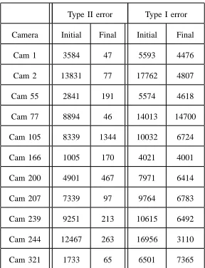
speed of computations. We computed re-projection errors: a Type II error (error of omission) and Type

I error (error of commission) by counts of voxels for several camera views used during our experiments

both after perturbation of the camera parameters and after evolution of the parameters as shown in Table 1.

After refinement stage, the Type I error dropped by 95%, and Type II error dropped by40%. As remarked

above, our goal is not to obtain absolute camera parameters but to help 3D reconstruction algorithm to

obtain objects correctly, which is achieved.

The Bust data comprises of numerous views, and this facilitated the following experiment to show the

used wrong camera calibration parameters, which belong to that of the neighbor views in the sequence in

Figure 16. This represents a possible perturbation in a real life scenario, i.e. the cameras are accidentally

moved a little bit after the calibration and the views that are captured afterwards are a little bit off. The

3D reconstruction of the Bust object on the top right shows the erroneous surfaces obtained in this case.

With our coordinated refinement of the extrinsic parameters using Eq.(28) and (33), the improvements in

the reprojection errors and the 3D reconstruction are observed in Figure 16.

A real color calibration experiment is carried out using HP Labs stereo rig system. We captured images,

shown in Fig.17, of the color calibration object from five cameras. Notice that the first picture is somewhat

darker than the others, second and third pictures appear lighter, and there is a color mismatch. A cube

surface is rigidly registered with the scene, also the radiance function on the cube is estimated as shown in

bottom row of Fig.17. The second row shows views after the evolution of color calibration coefficients are

completed. The third row shows the projections of the model surface onto the views. It can be visually

assessed that color responses of the cameras have achieved a balancing effect, and helped to obtain a

better texture mapping as well.

Next we demonstrate a calibration experiment using pictures from a handheld camera with no camera

calibration information available. In this scenario, the variational calibration techniques we presented

require some rough initial values that we obtained through a self calibration software currently under

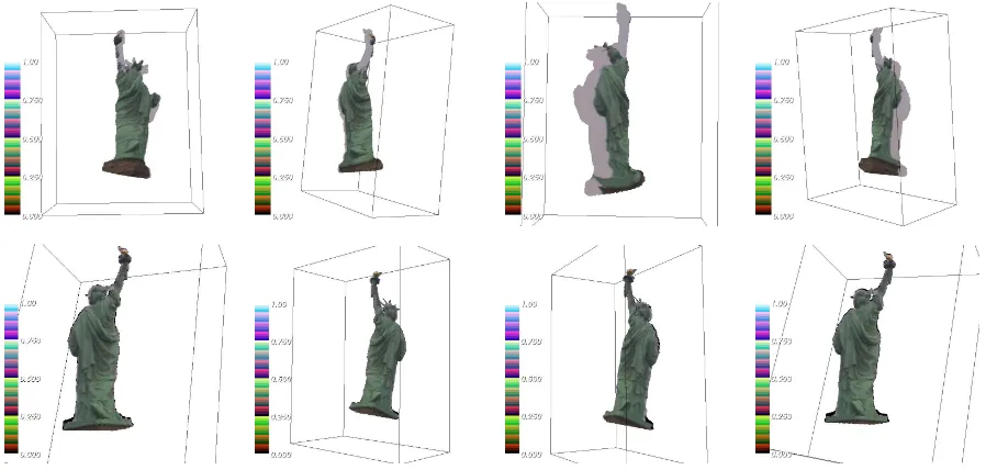
development. We have a 13 set of pictures taken around the Statue of Liberty, covering about 220/360

degrees of a circle around the statue, a few of the views shown in Figure 18.2 _{We obtained initial camera}

parameters: extrinsics and intrinsics including the skew parameter. A rough calibration results in the

projections shown in Figure 18. After evolution of the camera parameters: extrinsics, intrinsics including

the skew parameter, and color parameters, the comparison is done with the visual hulls of before and

after evolution camera parameters in Figure 19. One can observe the correction in the Statue of Liberty

surface with a better set of camera parameters obtained with the derived update equations throughout the

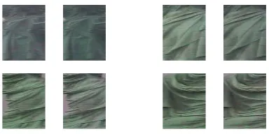
paper. We also show blow-up regions in Figure 20 from some of the camera views before and after the

evolution of the color camera parameters, and the colors are modified towards achieving some relative

agreement among the cameras which can however only be subjectively judged.

A. Discussions

One may argue that the requirement of some rough initial extrinsic and intrinsic camera parameters

limits the usability of this technique. However, the refinement or correction of camera parameters from a

perturbed state of a previous calibration is a real world problem that constantly presents obstacles to the

usage of multiple camera systems. After a very good initial calibration, the cameras over time may see

small changes in their parameters. For instance, extrinsic parameters will often be changed particularly

due to unwanted accidental motion. Similarly, the intrinsics and color parameters of the cameras may

go through small variations due to ambient conditions and wear-off. Therefore, the presented camera

calibration framework proves to be a useful tool for multi-camera systems.

B. Conclusions

In this paper, we employed the 3D stereo techniques based on variational ideas to various camera

calibration refinement problems. We have presented new multi-view stereo techniques to:

• evolve pose parameters of a 3D model object to take advantage of the known shape of calibration

object, and to reduce computational complexity,

• evolve distortion parameters of cameras given a 3D model shape,

• evolve color calibration parameters of cameras given a 3D model shape,

• evolve intrinsic parameters of cameras,

• evolve extrinsic parameters of cameras.

Pros and cons of this technique are discussed as follows:

• A nice feature of the methodology presented in this paper is that it can integrate several small and

different problems such as distortion calibration, color calibration into an overall unified system based

on the joint segmentation framework, and simultaneously evolve pose, color, distortion, extrinsic, and

• We make piecewise smooth object assumption and a constant background assumption, which may

be a limitation if the background is to be modeled as well. However, a background model may be

added to this framework if needed.

• The presented methods eliminate the need for search of image edges, point correspondences from

images, which can be very sensitive to pixel-level noise whereas our approach being based on image

regions for comparisons, is not as sensitive to noise.

• Another advantage of our framework is that it easily accommodates additional data. In the more

classical approaches to stereo, bringing in more data, or adding more images to the algorithm might

not help all the time, that is if something goes wrong in the independent segmentation phase of

even one image, it destroys the whole process of reconstructions and geometry. On the other hand,

adding more data to this joint segmentation framework will only improve robustness, providing more

tolerance towards errors.

• For the distortion calibration method, more improvements may be obtained with utilizing more poses,

hence many more camera images of the calibration object, and more than one distortion coefficient in

the model selected. One can also utilize more general/complicated distortion models than the simple

polynomial D function.

• Currently, we have an implicit representation of the calibration objects, i.e. the cube or the rectangular

bar. Computing surface normals, visibility functions for the surface occluding boundary from this

implicit representation is not perfectly exact, and the quantities are slightly smeared. A future direction

towards more efficient algorithms, is to use an explicit representation of the calibration object to more

accurately describe the occluding boundaries. With this approach, 3D grids are not needed for the

data structures, resulting in increased accuracy, speed and decreased memory requirements.

• Camera calibration is particularly suited to our framework, since it does not have to be done in

real-time, and also the environmental conditions may be allowed to vary to a degree (e.g. our choice

ACKNOWLEDGEMENTS

We acknowledge HP Labs, Palo Alto, CA, for their support to G. Unal and A. Yezzi through grants to Georgia Tech. for funding of this work. We thank our colleagues at HP Labs: Bruce Culbertson, Harlyn Baker, Irwin Sobel, Tom Malzbender, and Donald Tanguay for fruitful discussions and their support. We also thank Hailin Jin for providing us the Intel’s Bust dataset.

Fig. 3. Initialized surface model shown from three different vantage points.

Fig. 4. Column 1: Pose1. Row 1: one camera image shown, Row2: with projection of initialized surface (orange mask), Rows 3-5: during

evolution of the pose parameters of the surface, Row 6: with converged pose parameters. Columns 2-3: same as column 1 for poses 2 and

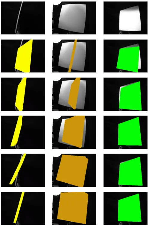
Fig. 5. Pose 1. Row 1: Three out of five captured views. Row 2: Projected surface after distortion parameters have converged. Row 3:

Undistorted with the obtained distortion coefficients.

Fig. 6. Pose 2. Row 1: Three out of five captured views. Row 2: Projected surface after distortion parameters have converged. Row 3:

Fig. 7. Pose 3. Row 1: Three out of five captured views. Row 2: Projected surface after distortion parameters have converged. Row 3:

Undistorted with the obtained distortion coefficients.

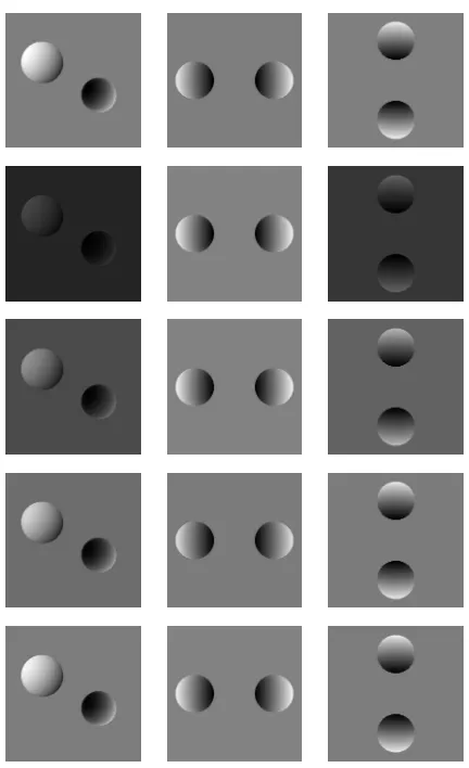
Fig. 8. Row 1: Three original views (cameras 1-7-9). Row 2: The same three different after deliberate simulated miscalibration of the

greyscales. The same three views while evolving the calibration parameters: Rows 3-4 intermediate stages, Row 5: The views after evolution

0 5 10 15 20 25 30 35 40 45 50 0.4 0.6 0.8 1 1.2 1.4 1.6 1.8 Alpha Evolution time Camera number: 0

0 5 10 15 20 25 30 35 40 45 50 0.4 0.6 0.8 1 1.2 1.4 1.6 1.8 Alpha Evolution time Camera number: 1

0 5 10 15 20 25 30 35 40 45 50 0.4 0.6 0.8 1 1.2 1.4 1.6 1.8 Alpha Evolution time Camera number: 2

0 5 10 15 20 25 30 35 40 45 50 0.4 0.6 0.8 1 1.2 1.4 1.6 1.8 Alpha Evolution time Camera number: 3

0 5 10 15 20 25 30 35 40 45 50 0.4 0.6 0.8 1 1.2 1.4 1.6 1.8 Alpha Evolution time Camera number: 4

0 5 10 15 20 25 30 35 40 45 50 0.4 0.6 0.8 1 1.2 1.4 1.6 1.8 Alpha Evolution time Camera number: 5

0 5 10 15 20 25 30 35 40 45 50 0.4 0.6 0.8 1 1.2 1.4 1.6 1.8 Alpha Evolution time Camera number: 6

0 5 10 15 20 25 30 35 40 45 50 0.4 0.6 0.8 1 1.2 1.4 1.6 1.8 Alpha Evolution time Camera number: 7

0 5 10 15 20 25 30 35 40 45 50 0.4 0.6 0.8 1 1.2 1.4 1.6 1.8 Alpha Evolution time Camera number: 9

Fig. 9. Evolution of the parameterαfor different camera views. Trueαvalue is shown as a dotted line.

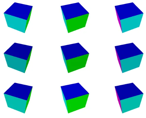
Fig. 10. Some camera views shown during the evolution of the color calibration. Top: original views, Middle: Perturbed views, Bottom:

Final views after convergence. Note the color similarity in top and bottom rows.

0 5 10 15 20 25 30 35 40 45 0 0.2 0.4 0.6 0.8 1 iterations alpha Camera 0

0 5 10 15 20 25 30 35 40 45 0 0.2 0.4 0.6 0.8 1 iterations alpha Camera 1

0 5 10 15 20 25 30 35 40 45 0.2 0.4 0.6 0.8 1 1.2 iterations alpha Camera 7

Fig. 11. Evolution of the parameterαfor different views for R,G,B channels of the synthetic color cube. Trueαvalue is shown as a dotted

0 50 100 150 350

360 370 380 390 400 410 420 430

iterations

focal length: x (−−), y(−.)

Camera 2

0 50 100 150 350

360 370 380 390 400 410

iterations

focal length: x (−−), y(−.)

Camera 5

0 50 100 150 360

370 380 390 400 410 420

iterations

focal length: x (−−), y(−.)

Camera 7

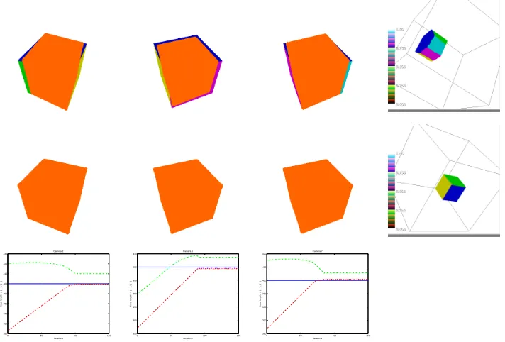
Fig. 12. Top: Three camera views shown during the evolution of the intrinsic parameters of an initial cube with projections from the initial

surface, Middle: Final views after convergence of the intrinsic parameters of the surface. Also shown at the bottom are the evolution of the

two focal length parameters for each shown camera view (red and green curves) along with the true (blue curve) focal lengths.

Fig. 13. Four camera views shown (top) during the evolution of the extrinsic parameters of an initial surface of a toy skater, Row 2:

Views shown with projections from the initial surface, Row 3: Final views after convergence of the extrinsic camera parameters. Visual hull

generated using the miscalibrated initial extrinsic parameters (row 2 right); visual hull generated using the converged extrinsic parameters

Fig. 14. Uncertainty ellipsoids drawn around each camera center for the toy skater data show the extrinsic refinement stability (right:

zoomed into one camera’s perturbations).

Fig. 15. Row 1: Four camera views during the evolution of the extrinsic plus intrinsic parameters of a toy skater with projections of

the initial surface, Row 2: Final views after convergence of the camera parameters. Visual hull generated using the miscalibrated initial

Type II error Type I error Camera Initial Final Initial Final

Cam 1 3584 47 5593 4476 Cam 2 13831 77 17762 4807 Cam 55 2841 191 5574 4618 Cam 77 8894 46 14013 14700 Cam 105 8339 1344 10032 6724 Cam 166 1005 170 4021 4001 Cam 200 4901 467 7971 6414 Cam 207 7339 97 9764 6783 Cam 239 9251 213 10615 6492 Cam 244 12467 263 16956 3110 Cam 321 1733 65 6501 7365

Table 1. Type I and Type II errors in counts of voxels for several camera views for Bust data (Fig. 16) after perturbation of camera parameters (Initial), and

after evolution of parameters (Final).

Fig. 16. Camera views 78,167, and 240 in top row are used deliberately with camera calibration parameters of camera views 77, 166, and

239 of the Van Gogh Bust dataset. Top: Three camera views shown with projections from the initial surface in row 2, here note the resulting

initial mismatch in projected silhouettes. Row 3: Final views after convergence of the camera parameters. Visual hull surfaces obtained by

using wrong calibration parameters for views 78, 167, 240 on the right (top row) and surfaces with corrected calibration parameters in bottom

Fig. 17. Some camera views shown during the evolution of the color calibration parameters of the HP color calibration object surface.

Top: Five camera views; Row 2: Final views after convergence of the extrinsic camera parameters; Row 3: Same shown with projections of

Fig. 18. Some camera views shown during the evolution of the camera calibration parameters of the Statue of Liberty surface. Top: Five

camera views shown with projections from the initial surface in Row 2; Row 3: Final views after convergence of the camera parameters.

Fig. 19. Visual hull surfaces with initial rough calibration parameters(top), and with refined calibration parameters (bottom), also with

Fig. 20. Some camera views before and after the color calibration for the statue of liberty.

REFERENCES

[1] O. Faugeras and R. Keriven, “Variational principles, surface evolution pdes, level set methods and the stereo problem,” Tech. Rep.,

INRIA, 1996.

[2] A. Yezzi and S. Soatto, “Stereoscopic segmentation,” Int. J. Computer Vision, vol. 53, pp. 31–43, 2003.

[3] A. Yezzi and S. Soatto, “Structure from motion for scenes without features,” in Proc. IEEE Conf. on Computer Vision and Pattern

Recognition, 2003, pp. 525–532.

[4] I. Sobel, “On calibrating computer controlled cameras for perceiving 3d scenes,” AI, vol. 5, pp. 185–198, 1974.

[5] R. Y. Tsai, “A versatile camera calibration technique for high-accuracy 3d machine vision metrology using off-the-shelf tv cameras

and lenses,” J. Robotics and Automation, vol. 3, pp. 323–44, 1987.

[6] R. Hartley and A. Zisserman, Multiple View Geometry in Computer Vision, Cambridge University Press, 2000.

[7] B. Triggs, “Camera pose and calibration from 4 or 5 known 3d points,” in Proc. IEEE Conf. on Computer Vision and Pattern

Recognition, 1999, pp. 278–284.

[8] P. Gurdjos and P. Sturm, “Methods and geometry for plane-based self-calibration,” in Proc. IEEE Conf. on Computer Vision and

Pattern Recognition, 2003, pp. 491–496.

[9] O.D. Faugeras, Q.T. Luong, and S.J. Maybank, “Camera self-calibration: Theory and experiments,” in Proc. European Conf. Computer

Vision, 1992, pp. 321–334.

[10] Y. Seo, A. Heyden, and R. Cipolla, “A linear iterative method for auto-calibration using the DAC equation,” in Proc. IEEE Conf. on

Computer Vision and Pattern Recognition, 2001, pp. 880–885.

[11] J. Oliensis, “Fast and accurate self calibration,” in Proc. Int. Conf. on Computer Vision, 1999, pp. 745–752.

[12] M. Pollefeys, R. Koch, and L. Van Gool, “Self-calibration and metric reconstruction in spite of varying and unknown intrinsic camera

parameters,” Int. J. Computer Vision, vol. 32, no. 1, pp. 7–25, 1999.

[13] T. Svoboda, D. Martinec, and T. Pajdla, “A convenient multi-camera self-calibration for virtual environments,” PRESENCE:

Teleoperators and Virtual Environments, vol. 14, no. 4, 2005.

[14] J. Heikkila and O.Silven, “A four-step camera calibration procedure with implicit image correction,” in Proc. IEEE Conf. on Computer

[15] G. Unal and A. Yezzi, “A variational approach to problems in calibration of multiple cameras,” in Proc. IEEE Conf. on Computer

Vision and Pattern Recognition, 2004, pp. 172–178.

[16] G. Unal, A. Yezzi, H. Baker, and B. Culbertson, “A variational approach to calibration of multiple cameras,” Tech. Rep., HP Labs,

HPL-2004-219, Palo Alto, CA, 2004.

[17] F. Devernay and O. Faugeras, “Straight lines have to be straight,” Machine Vision and Applications, vol. 13, pp. 14–24, 2001.

[18] J. Weng, P. Cohen, and M. Herniou, “Camera calibration with distortion models and accuracy evaluation,” IEEE PAMI, vol. 14, pp.

965–980, 1992.

[19] Z. Zhang, “A flexible new technique for camera calibration,” Tech. Rep., Microsoft Research, MSR-TR-98-71, 1998.

[20] D.C. Brown, “Decentering distortion of lenses,” Photogrammetric Engineering, vol. 32, 1966.

[21] M. T. El-Melegy and Aly A. Farag, “Nonmetric lens distortion calibration: Closed-form solutions, robust estimation and model

selection,” in Proc. Int. Conf. on Computer Vision, 2003, pp. 554–559.

[22] S.B. Kang, “Semiautomatic methods for recovering radial distortion parameters from a single image,” Tech. Rep., CRL Tech. Report

CRL 97/3, 1997.

[23] R. Swaminathan and S.K. Nayar, “Nonmetric calibration of wide-angle lenses and polycameras,” in Proc. IEEE Conf. on Computer

Vision and Pattern Recognition, 1999, pp. 2413–2418.

[24] G.P. Stein, “Lens distortion calibration using point correspondences,” in Proc. IEEE Conf. on Computer Vision and Pattern Recognition,

1997, pp. 602–608.

[25] A.W. Fitzgibbon, “Simultaneous linear estimation of multiple view geometry and lens distortion,” in CVPR, 2001.

[26] F. Du and M. Brady, “Self-calibration of the intrinsic parameters of cameras for active vision systems,” in Proc. IEEE Conf. on

Computer Vision and Pattern Recognition, 1993, pp. 477–482.

[27] H.S. Sawhney and R. Kumar, “True multi-image alignment and its application to mosaicing and lens distortion correction,” in Proc.

IEEE Conf. on Computer Vision and Pattern Recognition, 1997, pp. 450–456.

[28] H.H. Baker, D. Tanguay, I. Sobel, D. Gelb, M.E. Goss, B.W. Culbertson, and T. Malzbender, “The coliseum immersive teleconferencing

system,” Tech. Rep., HP Labs, HPL-2002-351, 2002.

[29] E. Marszalec, “On-line color camera calibration,” in Proc. Int. Conf. on Pattern Recognition, 1994, pp. 232–237.

[30] S. Osher and J.A. Sethian, “Fronts propagating with curvature dependent speed: Algorithms based on the Hamilton-Jacobi formulation,”

J. Computational Physics, vol. 49, pp. 12–49, 1988.

[31] D. Adalsteinsson and J.A. Sethian, “A fast level set method for propagating interfaces,” J. Computational Physics, vol. 118, pp.

269–277, 1995.

[32] J. Sokolowski and J.P. Zolesio, Introduction to Shape Optimization, Shape Sensitivity Analysis, Springer Verlag, Berlin, Heilderberg,

1992.