International Spillover and Rebound Effects from Increased Energy Efficiency in Germany

Increased energy efficiency in Germany:

International spillover and rebound effects

Simon Koesler,

Centre for European Economic Research

Kim Swales,

Department of Economics, University of Strathclyde

Karen Turner,

Centre for Energy Policy, University of Strathclyde

Making a difference to policy outcomes locally, nationally and globally

The views expressed herein are those of the author

and not necessarily those of the

International Public Policy Institute (IPPI)

,

International spillover and rebound effects

from increased energy efficiency in Germany

Simon Koesler, Kim Swales and Karen Turner

Abstract

The pollution / energy leakage literature raises the concern that policies implemented in one country, such as a carbon tax or tight energy restrictions, might simply result in the reallocation

of energy use to other countries. This paper addresses these concerns in the context of policies

to increase energy efficiency, rather than direct action to reduce energy use. Using a global Computable General Equilibrium (CGE) simulation model, we extend the analyses of ‘economy-wide’ rebounds from the national focus of previous studies to incorporate international spillover

effects from trade in goods and services. Our focus is to investigate whether these effects have

the potential to increase or reduce the overall (global) rebound of local energy efficiency improvements. In the case we consider, increased energy efficiency in German production

generates changes in comparative advantage that produce negative leakage effects, thereby

actually rendering global rebound less than national rebound.

JEL classifications:

D58; Q41; Q43; F18; Q56

Keywords:

Energy supply; energy demand; rebound effects; energy efficiency; general equilibrium; trade

spillover; energy and pollution leakage

1. Introduction

Existing research identifies the importance of trade effects on the nature and magnitude of

economy-wide rebound where domestic energy efficiency improvements have occurred (Hanley et al., 2009; Van den Bergh, 2011). Whilst Wei (2010) presents a theoretical analysis of ‘global rebound’ and there are a number of applied studies, including Barker et al. (2009), the

potential spillover effects from energy efficiency improvements in one nation on energy use in

other nations have generally been neglected (Madlener and Alcott, 2009; Sorrell, 2009;Turner,

This is an important knowledge gap, particularly given the global nature of energy-related

climate change and the existence of supra-national policy targets, such as the EU 20-20-20 framework. Potential interaction across geographic boundaries implies that energy efficiency

target setting and policy implementation decisions in different countries should be considered

as interdependent. This is of particular interest given the pollution leakage literature (e.g.

Babiker, 2005; Böhringer and Löschel, 2006; Löschel and Otto, 2009; Elliot et al., 2010), which

produces examples where environmental policies enacted in some countries simply result in

shifting the pollution generation or energy use to other countries. This pollution leakage typically

occurs through international changes in production and trade patterns. Here we relate the

leakage issue to policies that directly improve energy efficiency and consider the potential for both positive and negative leakage effects of energy efficiency improvements in one country on

energy use (and related emissions) in others (Baylis et al., 2014; Bento et al., 2012).

Specifically we investigate how the concept and treatment of economy-wide or 'macro-level'

rebound can be extended to take into account these wider impacts.

Rebound occurs when improvements in energy efficiency stimulate an increase in the direct

and/or derived demand for energy in production and final consumption. It is triggered by the

fact that an increase in energy efficiency increases the effective energy services gained from each physical unit of energy used. This reduces the price of energy, measured in efficiency (or

energy service) units (Berkhout et al., 2000; Birol and Keppler, 2000; Brookes 1990, 2000;

Greening et al., 2000; Herring, 1999; Jevons, 1865; Saunders, 1992, 2000a,b; Schipper and

Grubb, 2000; Van den Bergh, 2011). Recent reviews of the literature are given in Dimitropoulos

(2007), Sorrell (2007) and Turner (2013) whilst Maxwell et al., (2011) and Ryan and Campbell

(2012) provide policy-focussed reviews.

The economic impacts of increased energy efficiency in general, and rebound pressure in

particular, spread to the wider economy through a series of price and income effects. So-called ‘economy-wide’ rebound studies have generally been conducted in the context of improved efficiency in industrial energy use within individual national or regional economies. The most

common approach is to use multi-sector Computable General Equilibrium, CGE, models.

These are reviewed in Sorrell (2007) and more recent studies include Anson and Turner (2009)

and Turner and Hanley (2011). The aim of this paper is to augment this literature by extending

the spatial focus of the wider rebound effects using a multi-region CGE world model, developed

along the lines of the basic version of the WIOD CGE framework (Koesler and Pothen, 2013). 1

In Section 2, we consider the types of channel through which an efficiency improvement in productive energy use (i.e. within industries/production sectors rather than the household final

1_{This paper separately identifies all EU countries but treats the rest of the World (ROW) as a single}

consumption sector) in one nation can spill-over to impact energy use in direct and indirect trade

partners.2 _{In Section 3, we derive the analytical expressions required to extend the rebound}

calculation to incorporate endogenous changes in energy use at extended spatial levels. In

Section 4, we provide an overview of the world CGE framework that we use. This adopts the

type of specification commonly used to consider issues of pollution leakage resulting from

implementing environmental policies (e.g. Babiker, 2005; Böhringer and Löschel, 2006; Löschel

and Otto, 2009; Elliot et al., 2010). In Section 5, we outline the simulation strategy and in

Section 6 we present results from two sets of simulations. These are both for a 10% increase

in energy efficiency in production in the German economy. In one case this applies only to the “Manufacturing” sector. In the other, it applies in all production sectors. Results are reported for the change in key economic variables in Germany, the rest of the EU (REU) and the rest of

the world (ROW). Section 7 calculates a number of alternative rebound values for these

efficiency improvements. Section 8 draws conclusions and recommendations for future

research.

2. Extending the boundaries of the economy-wide rebound effect

2.1 Home Economy Effects

2.1.1. Energy efficiency improvements in a single sector

Where the energy efficiency improvement applies to only one (target) sector, the

home-economy impacts that affect rebound operate through the following channels. First, there is

substitution towards energy, measured in efficiency units, in production in the target sector.

This operates through the fall in the price of energy used in production in that sector, when that

energy is measured in efficiency units. This means that the proportionate fall in energy use, now measured in natural units, per unit of output in that sector is less than the efficiency

improvement. The second channel is the increased competitiveness of the target sector. This

is driven by the reduced costs associated with the reduced intermediate input use. Both the

substitution and competitiveness effects increase the rebound value. A third channel is the

reduction in energy use through the energy sector supply chain. Energy production is energy

intensive. A reduction in demand for energy in the target sector will further reduce the demand

for energy in the production of energy itself. This third channel reduces the rebound value.

Additional home-economy impacts are driven by the changes in the general use of energy as

an intermediate input to supply production and also to directly meet changes in consumption

demand. As argued already, we expect the output of the target sector to rise and output in the

2 _{Lecca et al. (2014) investigate the economy-wide impacts of increased efficiency in household energy}

energy sector to fall (as long as there is no ‘backfire’, i.e. rebound greater than 100%). However,

the actual composition of output across other sectors will depend on the sectoral reallocation of the fixed factors, capital and labour, driven by the adjustments to factor prices. These changes

in factor prices, together with the change in the technology in the target sector, are reflected in

all commodity prices which are determined simultaneously in equilibrium. These prices drive

the relative competitiveness of the sectors and, together with the composition and price

sensitiveness of final demands, will act to further impact economy-wide rebound.

2.1.2. An energy efficiency gain in all sectors

Where the energy efficiency gain applies to all sectors, there will be the same home economy substitution effect leading to increased energy use in production, when measured in efficiency

units. This now operates in all sectors and remains a major channel for rebound. However, the

ultimate size of the competitiveness effect for individual sectors will be affected by their energy

intensity. It is clearly the case that with fixed, fully-employed, factors of production output cannot

rise in all sectors simultaneously. The price of factors in general will increase (although there

will normally also be distributional effects). Therefore, some sectors will actually lose

competitiveness, even though their energy efficiency has risen. However we expect that the

more energy intensive sectors will experience the bigger cost reductions and, therefore, ultimately be those that are more competitive after the efficiency increase. In this respect, it is

important to note that energy itself is a highly energy intensive sector, so that it is likely to be

one of the sectors whose competitiveness increases.

2.2 Foreign Economy Effects

In all cases the economies of countries that do not directly experience an improvement in energy efficiency are affected through three channels. Two of these relate to changes in trade-related

demand (the changes in exports and import substitution). The third is the accompanying

changes in intermediate and consumption demand.

The changes in trade-related demand are determined through competitiveness and composition of demand channels. The relative competitiveness effects are primarily governed by price

changes in the home economy. If the price falls in a particular home sector, we expect that the

competitiveness of the corresponding sector in other countries will fall with an accompanying

negative impact on output. Similarly, if the composition of home-country import demand

changes for non-price reasons, this affects the export demand in foreign countries. Such a

demand change would include shifts in energy demand directly affected by the increased

However, it is important to note that the changes in foreign energy exports or import substitution

do not directly affect energy use in foreign countries. If more energy is exported this means that the energy is to be used elsewhere. However, the third, supply-chain, channel is important

in this respect. This is the change in intermediate demands that accompanies the changes in

trade-related demands.

There are additionally other general equilibrium impacts but these are likely to be less important.

There are possible changes in the energy intensity of production that would accompany

changes in relative energy prices. Similarly, if consumption demand increases through

favourable changes in the terms of trade, this will affect energy demand. However, we expect the primary impact to come through changes in intermediate demand driven by changes in the

size and composition of export demand.

3. Quantifying rebound in a multi-regional setting

Here we build on the economy-wide rebound specifications derived in Lecca et al. (2014) to

consider the general equilibrium rebound effects of a proportionate improvement in the

efficiency with which energy is used in a single production sector. Own-sector rebound in the

targeted sector i, is identified as 𝑅𝑖, and is reported in percentage terms. It implicitly

incorporates general equilibrium feedback effects on sector i’s energy use, in addition to direct

and indirect rebound effects. It is defined as:

𝑅𝑖= [1 +

𝐸𝑖̇

𝛾] 100, (1)

where 𝐸𝑖̇ is the change in energy use in sector i after all agents have adjusted their behaviour

in consequence of the technical energy efficiency improvement,





0

efficiency improvement,



To reiterate, this is not direct rebound; rather it is the rebound calculated incorporating the change in energy use in sector i with all general equilibrium effects of the efficiency improvement

taken into account.

The first step in identifying the own-country economy-wide rebound effect is to consider the

impact of the proportionate energy efficiency improvement in the treated sector i on total energy

The own-country total production rebound formulation, 𝑅𝑝, is given as:

𝑅𝑝= [1 +

𝐸𝑝̇

𝛼𝛾] 100, (2)

where  is the initial (base/reference year) share of sector i energy use in total energy use in

production (across all i=1,…,N sectors) in the domestic economy. The term 𝐸𝑝̇ 𝛼𝛾⁄ can be

expressed as:

𝐸𝑝̇

𝛼𝛾= ∆𝐸𝑝

𝛾𝐸𝑖 =

∆𝐸𝑖+ ∆𝐸𝑝−𝑖

𝛾𝐸𝑖 =

𝐸𝑖̇

𝛾 + ∆𝐸𝑝−𝑖

𝛾𝐸𝑖 ,

(3)

where  represents absolute change and the -i superscript indicates all production excluding

sector i. Substituting equation (3) into equation (2) and using equation (1) gives:

𝑅𝑝= 𝑅𝑖+ [

∆𝐸𝑝−𝑖

𝛾𝐸𝑖 ] 100. (4)

This shows that the total (own-country) rebound in productive energy use will be greater than

the own-sector rebound if there is a net increase in aggregate energy use across all other

domestic production sectors. On the other hand, if there is a net decrease in total energy use

across these sectors, then total rebound in production will be lower than own-sector rebound.

Using a similar procedure, detailed in Appendix A, we can show that the full economy-wide rebound effect in the domestic economy, Rd, can be expressed as:

𝑅𝑑= 𝑅𝑝+ [

∆𝐸𝑐

𝛾𝐸𝑖] 100. (5)

where the c subscript indicates 'consumption' (households). Equation (5) indicates that the total

economy-wide rebound in the home country, d, will be larger (smaller) than rebound in the

aggregate production sector if there is a net increase (decrease) in energy use in household

final consumption.

In this paper we are particularly interested in the international energy-use spill-over effects. Therefore, we define a global rebound effect, 𝑅𝑔, relating to the total impact on energy use in

economy, d. Again, adopting a similar approach, outlined in Appendix A, this can be expressed

as:

100

d g

g d

i

E

R

R

E













_{ }

_









where

E

shock. Again, expression (6) shows that the total economy-wide global rebound will be greater

than the own-country rebound if there is a net increase in external aggregate energy use following the efficiency improvement within country d. If there is a net decrease then total global

rebound will be lower than own-country rebound. Note that it is possible to identify more than

one region within the external global economy and disaggregate the changes in global

non-domestic energy use accordingly. We do this below in our case study of increased efficiency

in German industrial energy use by separately identifying the change in energy use in the rest

of the EU-27 and the rest of the world.

4. The global CGE modelling framework

To evaluate the economy-wide rebound and provide a first analysis of the full international

spill-over effects that accompany an increase in domestic energy efficiency, we make use of a static, multi-region, multi-sector CGE world model which has been developed along the lines of the

Basic WIOD CGE (Koesler and Pothen, 2013). In the present analysis the model feature 28

separate regions. These comprise all the individual EU27 member states and Rest of the World

(ROW). However, for ease of exposition, in presenting the simulation results we aggregate the

outcomes for all EU member states apart from Germany, so that we report figures for Germany

(GER), the Rest of the EU (REU) and the Rest of the World (ROW).

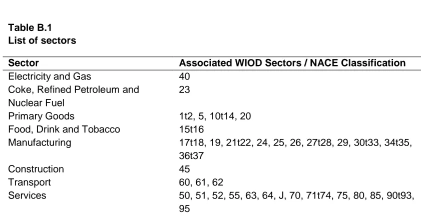
The model disaggregates production to eight sectors/commodities. Two are energy supply sectors/commodities: “Electricity and Gas” and “Coke, Refined Petroleum and Nuclear Fuel”. The other six (non-energy supply) sectors/commodities are “Primary Goods”, “Food, Drink and Tobacco”, “Manufacturing”, “Construction”, “Transport” and “Services”. The mapping of these aggregate sectors to the original WIOD sectors is given in Table B.1 in Appendix B.

The production of each commodity is characterised by a KLEM production structure shown in

Figure 1, which features a CES function at every level. Capital, K(r), and labour, L(r), enter the

energy composite is a (fixed coefficients) Leontief aggregation comprising the commodities “Electricity and Gas” and “Coke, Refined Petroleum and Nuclear Fuel”. On the top level the energy-value-added composite is combined with a non-energy material aggregate A(neg,r) to

create the sector gross output, Y(i,r).3. The intermediate composite is also a Leontief aggregation

of all six non-energy commodities identified above. Sectoral output can be used for intermediate

use, final domestic consumption or exported. Commodities are made up of composites of the

domestic production and imports, using the Armington (1969) assumption of incomplete

substitution.

Each region has one aggregated representative agent who supplies a fixed amount of capital and labour. Both factors are immobile between regions but completely mobile across sectors

within each region. All factors are fully employed, which determines the relevant wage and

capital rental payments. This implies a Marshallian long-run interpretation of the simulation

results, in that in each equilibrium all factor use is fully adjusted to the ruling factor and

commodity prices.

The consumption decision of the representative agent embraces all the household and

governmental (private and public) final demand in a region. The representative agent maximizes her utility by purchasing bundles of consumption goods subject to a budget

constraint. The budget is determined by factor and tax income along with interregional

borrowing or saving. The utility of representative agents U(r) is given as a Leontief composite

of energy A(eg,r) and a non-energy commodities A(neg,r). The structure of the utility functions is

shown in Figure 2.4

Figure 1: Structure of commodity production Figure 2: Structure of utility function

3 _{There are other ways of structuring the nested KLEM production function and there are also other}

possible functional forms (Lecca et al., 2011). Alternative CES structures and functional forms will be investigated in future work.

4 _{Modelling consumption on the basis of a Leontief function is restrictive, although it has recently been}

Regarding the basic economic structure, the model builds on data from the World Input-Output

Database (WIOD) (Timmer et al., 2012; Dietzenbacher et al. 2013) and is calibrated to the year

2009.5 _{The structure of the Armington trade aggregation is shown in Figure 3, with the}

corresponding Armington elasticities taken from GTAP7 (Badri and Walmsley, 2008; Hertel et

al., 2007; Hertel et al., 2008). For substitution elasticities determining the flexibility of production

with regard to inputs, we turn to estimates from Koesler and Schymura (forthcoming).6 _Savings

and borrowing are not directly reported in WIOD but they result from the imbalance of final

demand and factor endowments or other sources of revenue (taxes, emission allowances, etc.).

Overall macroeconomic balance is achieved by changes in interregional savings/borrowing,

whilst the overall savings and borrowing of final demand agents are held constant. Prices are

expressed against the numeraire which is taken to be the consumer price index (CPI) for the

rest of the World.

Figure 3: Structure of Armington aggregate

5. Simulation strategy

We wish to simulate the impact of the adoption of energy-saving technological change in

production. As is standard in rebound studies, we assume that this technological change is

supplied as a public good. This implies that the efficiency improvement is assumed to be

costless in two respects. First, resources are not required to create the knowledge on which

the efficiency improvement is based. Second, firms can implement the efficiency changes

without using additional resources. We make these assumptions because the study of rebound

focusses on the difference between actual and expected energy saving from the introduction of improved energy efficiency. It is the reduced cost of energy in efficiency units which drives the

5 _{The WIOD database is available at http://www.wiod.org. We use data downloaded on the 17}th _{of April}

2013.

6 _{Koesler and Schymura (forthcoming) fail to provide substitution elasticities between capital and labour}

rebound effects. The simulations attain maximum transparency if the efficiency improvements

are assumed to be costless. It is important to distinguish the rebound effect associated with pure efficiency improvements from the wider impact of policies, such as carbon pricing or cap

and trade schemes, which achieve a reduction in the use of energy only through the use of

previously more costly other inputs.7

We therefore follow the common procedure adopted in CGE studies of economy-wide rebound

by examining the effects of an exogenous step increase in the efficiency of energy used as an

intermediate input. We consider two scenarios. In both, we apply a 10% technical improvement

in German energy efficiency in production.8 _{In the first simulation this applies solely to the}

“Manufacturing” sector. In the second scenario, the energy efficiency stimulus is experienced by all eight German production sectors. In each case, the new post-shock equilibrium is then

compared to the original equilibrium (without the efficiency changes) and the appropriate

rebound values are calculated. This therefore represents a comparative static analysis in which

all changes can be attributed to the efficiency shock.9

The energy efficiency shock is applied to the second nest of the treated sectors’ production

functions (see Figure 2) which take the form:

𝐶𝐸𝑆_{𝐾𝐿𝐸(𝑖,𝑟)}𝐾𝐿𝐸𝑀 _{= (𝜂} 𝐾𝐿(𝑖,𝑟) 𝐾𝐿𝐸 _{(𝐶𝐸𝑆}

𝐾𝐿(𝑖,𝑟)𝐾𝐿𝐸 ) 𝜌_(𝑖,𝑟)𝐾𝐿𝐸

+ 𝛾_(𝑖,𝑟)𝐸𝑛𝑒𝑟𝑔𝑦𝜂_{𝐸(𝑖,𝑟)}𝐾𝐿𝐸 _(min 𝑒𝑔 (

𝐴(𝑒𝑔,𝑟)

𝜂_{(𝑒𝑔,𝑟)}𝐸 )) 𝜌_(𝑖,𝑟)𝐾𝐿𝐸

)

1 𝜌_(𝑖,𝑟)𝐾𝐿𝐸

, (7)

where, η are input shares, ρ are substitution parameters and γEnergy _{indicates the level of energy}

efficiency which is normalised to be one in the initial equilibriium. The proportionate change in

demand for intermediate energy use would apply equally between domestic and imported

electricity as long as relative electricity prices remained the same. In the first scenario the

efficiency parameter,



German “Manufacturing” sector only. In the second scenario, the parameter is increased across

all German production sectors.

7_{However, the issue of the costs associated with efficiency improvements is one that is often raised in}

discussions of simulating efficiency changes. This is addressed in more depth in Appendix C.

8 _{On average the energy efficiency of the German industry has increased by about 1.6% per annum}

(BMWi, 2013). In the process of our analysis, we also considered efficiency improvements of 5%, 20% and 30%. But as the magnitude of the shock only affects the scale of the different effects and does not change the underlying basic effects. Here we report findings which would correspond to just over 5 years worth of technical improvement, mapping to an energy efficiency improvement of 10%.

9 _{In future work we aim to consider more sophisticated ways of simulating efficiency improvements, for}

It is useful to give an indication of the size of shock that is to be given to the international

economy through these efficiency changes. Table 1 shows the energy used in German “Manufacturing” and in German production as a whole as a share of total energy use in German production, the German economy as a whole, the combined EU and the world economy.10 _The

data show that the energy use in “Manufacturing” makes up 28.58% of the total energy used in

German production. Energy used in German production is 57.99% of total German domestic

energy use, and 10.81% and 2.95% of all EU and World energy use. It is clear that we would expect energy efficiency improvements in German “Manufacturing” and in German production

as a whole to have impacts which would spread outwith the German national border.

Table 1

The energy used in German “Manufacturing” and German production expressed as a percentage of total energy used in German production, and the German, EU and World economies.

German production (α)

German economy (β)

EU economy (φ)

World economy (χ) German

“Manufacturing”

28.58 16.57 3.09 0.84

German Production 100.00 57.99 10.81 2.95

Source: Authors’ calculations based on WIOD,

(Timmer et al., 2012; Dietzenbacher et al., 2013)

6. Impacts of a 10% increase in energy efficiency in the German “Manufacturing” sector and in all German production

6.1 Simulation 1: 10% increase in energy efficiency in German “Manufacturing”

In this sub-section we consider the effects of an energy efficiency improvement, targeted on the German “Manufacturing” sector. The percentage impacts on key aggregate and sectorally

disaggregated variables for the German, rest of the EU (REU) and rest of the world (ROW)

economies are reported in Tables 2 and 3. The absolute change in sectoral outputs for the

same geographical areas are given in Table 4.

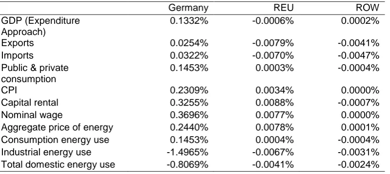
It is useful to begin by considering the impact on the German economy, as this is where the direct shock occurs. As expected, there is an increase in GDP (0.1332%) which is reflected in

10_{These proportions are also required for the calculation of the rebound values using equations (2), (A3)}

the increase in the returns to capital and labour. However, these effects are small, driven by

the limited scope of the efficiency improvement. The increase in the real wage, calculated as the percentage change in the nominal wage minus the percentage change in the CPI, is

0.1387%, whilst the increase in the real payment to capital, calculated in a similar way, is less

at 0.0946%. Total consumption rises, broadly in line with GDP and incomes, and both

aggregate exports and imports also increase. Energy use in public and private consumption

increases at the same rate as total consumption; that is by 0.1453%, which reflects the fixed

coefficients assumed in the consumption function.11 _{However, the industrial use of energy falls}

by 1.4965% driven primarily by the fall in energy use in “Manufacturing”. As a result, total

domestic energy use declines by 0.8069%.

Table 2

Change in key macroeconomic indicators

Scenario 1: 10% increase in energy efficiency in German manufacturing

Germany REU ROW

GDP (Expenditure Approach)

0.1332% -0.0006% 0.0002%

Exports 0.0254% -0.0079% -0.0041%

Imports 0.0322% -0.0070% -0.0047%

Public & private consumption

0.1453% 0.0003% -0.0004%

CPI 0.2309% 0.0034% 0.0000%

Capital rental 0.3255% 0.0088% -0.0007%

Nominal wage 0.3696% 0.0077% 0.0000%

Aggregate price of energy 0.2440% 0.0078% 0.0001%

Consumption energy use 0.1453% 0.0004% -0.0004%

Industrial energy use -1.4965% -0.0067% -0.0031% Total domestic energy use -0.8069% -0.0041% -0.0024%

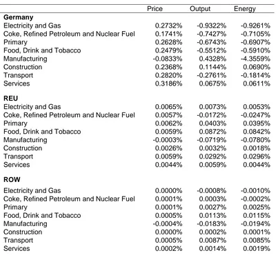
To get more detail as to the factors underpinning these results, it is useful to turn to Tables

3 and 4 which give sectorally disaggregated information. Again we focus initially on the figures for the German economy. The impact on prices is very clear: “Manufacturing” prices exhibit a

small reduction of 0.0833%, reflecting the direct improvement in technical efficiency, whilst the

prices in all other sectors rise within the range 0.1741% and 0.3186%, in line with the increases

in nominal wages and capital rentals.12

11 _{This is subject to sensitivity analysis in Appendix Tables B2 and B3.}

12 _{Recall that the numeraire is the CPI in the rest of the world. The reported price changes are therefore}

The accompanying impact on sectoral outputs is similarly quite clear cut. From Table 4 it is apparent that there is a relatively large increase in output in “Manufacturing” of $6.6314 billion (0.4328%). This is stimulated by a rise in exports, import substitution and increased domestic income as “Manufacturing” goods become relatively cheap. There are also increases in output in other sectors that mainly supply the domestic (public and private) consumption, with an expansion in the “Service” and “Construction” sectors.. However, output falls in the energy sectors (“Electricity and Gas” and “Coke, Refined Petroleum and Nuclear Fuel”) again primarily

as a result of the direct improvements in energy efficiency, plus there are falls in other sectors more dependent on foreign trade, such as the “Food, Drink and Tobacco”, “Transport” and “Primary” sectors. In total, output increases by $5.0016 billion.

Table 3

Changes in sectoral price, output and energy use

Scenario 1: 10% increase in energy efficiency in German “Manufacturing”

Price Output Energy

Germany

Electricity and Gas 0.2732% -0.9322% -0.9261%

Coke, Refined Petroleum and Nuclear Fuel 0.1741% -0.7427% -0.7105%

Primary 0.2628% -0.6743% -0.6907%

Food, Drink and Tobacco 0.2479% -0.5512% -0.5910%

Manufacturing -0.0833% 0.4328% -4.3559%

Construction 0.2368% 0.1144% 0.0690%

Transport 0.2820% -0.2761% -0.1814%

Services 0.3186% 0.0675% 0.0611%

REU

Electricity and Gas 0.0065% 0.0073% 0.0053%

Coke, Refined Petroleum and Nuclear Fuel 0.0057% -0.0172% -0.0247%

Primary 0.0062% 0.0403% 0.0395%

Food, Drink and Tobacco 0.0059% 0.0872% 0.0842%

Manufacturing -0.0003% -0.0719% -0.0780%

Construction 0.0026% 0.0032% 0.0018%

Transport 0.0059% 0.0292% 0.0296%

Services 0.0044% 0.0059% 0.0044%

ROW

Electricity and Gas 0.0000% -0.0008% -0.0010%

Coke, Refined Petroleum and Nuclear Fuel 0.0001% 0.0003% -0.0002%

Primary 0.0001% 0.0027% 0.0025%

Food, Drink and Tobacco 0.0005% 0.0113% 0.0115%

Manufacturing -0.0004% -0.0183% -0.0194%

Construction 0.0000% 0.0002% 0.0001%

Transport 0.0005% 0.0087% 0.0085%

As we indicate earlier, it is important to understand the impact on Germany, as this is the country

that receives the direct economic shock. However, in this paper we are equally, if not more, concerned with the effect on the economies of the rest of the European Union (REU) and the rest of the World (ROW). Of particular interest is the change in energy use outwith Germany’s boundaries.

Table 4

Changes in output [Billion 2009 USD]

Scenario 1: 10% increase in energy efficiency in German ”Manufacturing”

Germany REU ROW World

Regional total 5.002 -0.860 -1.973 2.169

Electricity & Gas -1.579 0.054 -0.016 -1.541 Coke, Refined Petroleum and Nuclear Fuel -0.526 -0.063 0.005 -0.584

Primary -0.683 0.315 0.200 -0.168

Food, Drink and Tobacco -0.940 0.824 0.424 0.308

Manufacturing 6.631 -3.124 -3.422 0.085

Construction 0.337 0.065 0.010 0.412

Transport -0.424 0.245 0.255 0.076

Services 2.186 0.825 0.571 3.582

It is instructive to begin by considering Table 4. The efficiency improvement in Germany

increases world output by $2.169 billion. German output increases by $5.002 billion, but there

are reductions in the aggregate value of output in REU and ROW of $0.860 and $1.973 billion

respectively. The German sector most strongly affected by the efficiency improvement is the one directly targeted with the shock, “Manufacturing”, and the increase in its competitiveness has an important direct impact on the REU and ROW economies. In particular, Table 4 indicates that the $6.631 billion expansion in output in German “Manufacturing” essentially simply displaces “Manufacturing” output in REU and ROW, which fall by $3.124 billion and $3.422 billion respectively. The shift of resources out of “Manufacturing” means that in REU

and ROW economies the output in almost all other sectors increases. In both countries the biggest absolute increase in output is in “Services”. However, there are also large increases in “Food, Drink and Tobacco”, “Transport” and in the “Primary” sectors, which experience a decline in output in Germany. Clearly crowding out in these sectors in Germany leads to expansion in

the rest of these external economies.

In Germany there is an increase in both the real wage and the capital rental rate, with the wage

increasing more rapidly. With the REU and ROW economies the situation is rather different. In

the REU there is an increase in the real return to both factors, but in this case the capital rental

consumption of energy also increases. However, the rise in the real price of energy, together

with the sectoral shifts in the composition of output means that the use of industrial energy falls. In REU, output in the “Electricity and Gas” sector rises but in “Coke, Refined Petroleum and Nuclear Fuel” output falls and total domestic energy use declines.

In the rest of the World (ROW), Table 2 shows that the wage is constant and the capital rental

falls. ROW private and public total consumption and consumption of energy decline in line.

Again the real price of energy rises and total industrial and domestic energy use fall. In this case the production of “Electricity and Gas” falls but “Coke, Petroleum and Nuclear Fuel” rises.

6.2 Simulation 2: 10% increase in energy efficiency in all German sectors

In this simulation we introduce an across the board 10% improvement in energy efficiency in

production in all German sectors. The effects on key aggregate and sectorally disaggregated

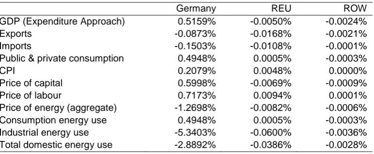
economic variables are reported in Tables 5, 6 and 7. The first key point from Table 5 is that,

as we would expect, the size of the response to the supply-side shock to the German economy

is much larger than in Simulation 1. German GDP increases by 0.5159%, the increase in the real returns to labour and capital are 0.5094% and 0.3919% respectively and private and public

consumption increases by 0.4948%. However, the proportionate changes in REU and ROW

variables are still low, and this is especially important for prices, where the change are small

relative to the those that occur in Germany. Recall that the ROW CPI is taken as the numeraire

and therefore remains unchanged and the increase in the REU CPI is 0.0034% as against the

increase in Germany of 0.2309%.

Table 5

Change in key macroeconomic indicators

Scenario 2: 10% increase in energy efficiency across all German sectors

Germany REU ROW

GDP (Expenditure Approach) 0.5159% -0.0050% -0.0024%

Exports -0.0873% -0.0168% -0.0021%

Imports -0.1503% -0.0108% -0.0001%

Public & private consumption 0.4948% 0.0005% -0.0003%

CPI 0.2079% 0.0048% 0.0000%

Price of capital 0.5998% -0.0069% -0.0009%

Price of labour 0.7173% 0.0094% 0.0001%

Price of energy (aggregate) -1.2698% -0.0082% -0.0006% Consumption energy use 0.4948% 0.0005% -0.0003% Industrial energy use -5.3403% -0.0600% -0.0036% Total domestic energy use -2.8892% -0.0386% -0.0028%

and import intensities. From the figures in Table 6, we observe that the biggest reductions in price occur in the energy sectors themselves, “Electricity and Gas” and “Coke, Refined Petroleum and Nuclear Fuel”. This is not primarily because of changes in demand for the output of these sectors but rather because these sectors are themselves very energy intensive in

production.13 _{The increase in energy efficiency therefore has a particularly marked impact on}

their prices. Other sectors where prices fall are “Transport”, “Primary” and “Food, Drink and Tobacco”. Note that in the labour intensive “Services”, “Construction” and “Manufacturing”

sectors, prices rise.

Table 6

Changes in sectoral price, output and energy use

Scenario 2: 10% increase in energy efficiency across all German sectors

Price Output Energy

Germany

Electricity and Gas -1.4237% -1.9661% -6.8403%

Coke, Refined Petroleum and Nuclear Fuel -0.9062% -0.5980% -5.0356%

Primary -0.2409% 0.7805% -4.7481%

Food, Drink and Tobacco -0.0937% 0.5278% -6.5592%

Manufacturing 0.0165% 0.0199% -4.0749%

Construction 0.2112% 0.4154% -7.2741%

Transport -0.3782% 0.6551% -2.9632%

Services 0.3914% 0.2978% -5.9916%

REU

Electricity and Gas -0.0052% -0.1858% -0.1990%

Coke, Refined Petroleum and Nuclear Fuel -0.0040% -0.3649% -0.3819%

Primary 0.0018% -0.0860% -0.0768%

Food, Drink and Tobacco 0.0024% -0.0142% -0.0106%

Manufacturing 0.0048% 0.0278% 0.0516%

Construction 0.0060% 0.0017% 0.0075%

Transport 0.0056% -0.0506% -0.0369%

Services 0.0063% 0.0097% 0.0200%

ROW

Electricity and Gas -0.0007% -0.0350% -0.0335%

Coke, Refined Petroleum and Nuclear Fuel -0.0005% -0.0381% -0.0366%

Primary -0.0004% -0.0215% -0.0199%

Food, Drink and Tobacco -0.0004% -0.0026% -0.0015%

Manufacturing 0.0001% 0.0122% 0.0167%

Construction 0.0001% 0.0001% 0.0011%

Transport -0.0004% -0.0159% -0.0152%

Services -0.0001% 0.0029% 0.0050%

Output falls in the two energy sectors but increases in all others. The proportionate figures reported in Table 6 are slightly misleading: from Table 7 we observe that the sector that has the

13 _{Changes in demand for a commodity only affect its price in this long-run model in so far as they change}

second smallest (0.2978%) proportionate increase in output, “Services”, has the largest ($9.647

billion) absolute increase. The 0.4948% rise in domestic consumption demand is driving this change in “Service” output and the increase in the output in this sector requires resources to be shifted from other sectors. We know that the energy sectors will release resources and the relatively small increase in output in “Manufacturing” implies that resources will be released

here too. In this simulation, overall both German exports and imports fall, so that the increase

in activity involves import substitution. Domestic private and public consumption of energy

increases by 0.4948% but this is completely dominated by the 5.3403% fall in industrial energy

use, so that total domestic energy use declines by 2.8892%.

Table 7

Changes in output [Billion 2009 USD]

Scenario 2: 10% increase in energy efficiency across all German sectors

Germany REU ROW World

Regional total 10.117 -1.311 -0.065 8.741

Electricity & Gas -3.331 -1.364 -0.713 -5.408 Coke, Refined Petroleum and Nuclear Fuel -0.423 -1.326 -0.648 -2.397

Primary 0.791 -0.672 -1.587 1.468

Food, Drink and Tobacco 0.900 -0.134 -0.099 0.667

Manufacturing 0.305 1.210 2.286 3.801

Construction 1.222 0.035 0.006 1.263

Transport 1.006 -0.424 -0.469 0.113

Services 9.647 1.364 1.158 12.169

The sectoral responses from both the REU and ROW economies are, in this case, qualitatively

similar. Total output summed across all sectors falls in both regions: by $1.311 billion in the

REU and by $0.065 billion in ROW. There are reductions in output in the two energy sectors,

reflecting both the lower industrial demand in Germany plus the increased competitiveness of the German energy sectors. These output reductions in the REU and ROW energy sectors are

less, in absolute terms, than the corresponding declines in Germany. However, they make up

almost 40% of the world reduction in the energy output resulting from the improvement in

German energy efficiency. Also these energy sectors are the sectors generally showing the largest absolute reductions in output in REU and ROW. Only the “Primary” sector in the ROW

registers a bigger fall.

In the “Services”, “Construction” and “Manufacturing” sectors, REU and ROW output increases in line with the expansions in the German economy. In Germany these are sectors that

“Primary” sectors show reductions in REU and ROW outputs which are moving contrary to the

changes in German output. These are REU and ROW sectors which are now less competitive than their German counterparts.

The proportionate impact on aggregate variables in REU and ROW is shown in Table 5. Both

aggregate exports and imports are reduced for REU and ROW. There is a small rise (0.0005%) in public and private consumption in REU but a small proportionate fall of 0.0003% in ROW. In

both regions, the real wage rises and the real return on capital falls. This change in the relative

factor prices is particularly marked in REU. Clearly capital released from the energy sectors is

difficult to reabsorb in the expanding sectors driven by increased German consumption

demand. In REU, private and public consumption of energy increases but this is dominated by

the reduction in production, so that total domestic energy use falls by -0.0386%. In ROW,

energy use in both private and public consumption and in industry falls, with total ROW domestic energy use declining by -0.0028%.

7. Rebound calculations

7.1 Scenario 1: a 10% increase in energy efficiency in German “Manufacturing”

The figures in column 3 of Table 3 give the sectorally disaggregated proportionate changes in energy use that result from the 10% increase in energy efficiency in the German “Manufacturing”

sector. The first point to note is that the actual reduction in energy use in German “Manufacturing” is 4.3559%. Using equation (1), this translates to an own-sector rebound value,

Ri, of 56.44%. However, recall that this is not limited to direct rebound in that it incorporates all

the general equilibrium effects that impact on this sector. This value, and all the other rebound

values, are given in Table 8.

Table 8

General equilibrium rebound effects for Scenarios 1 (10% increase in energy efficiency in German “Manufacturing”) and Scenario 2 (10% increase in energy efficiency across all German sectors)

Own-sector Ri

Own-country production Rp

Own-country total Rd

Global EURg WorldRg

Scenario1

Rebound [%] 56.44 47.63 51.31 50.22 48.11

Change [% points]

-8.81 3.68 -1.09 -2.11

Scenario 2 Rebound [%] Change [% points]

n.a 46.60 50.18

3.58

47.28 -2.90

46.58 -0.70

The primary interest of this paper is to investigate how rebound values change as the scope of

other (consumption) uses and other economies. It is sometimes implied that such increases in

scope will necessarily increase the rebound value. Our results show that this is not the case.

The first extension is to include the use of energy in production in the other German sectors, so

as to calculate the own-country production rebound value, Rp. Equation (4) shows that the

measured rebound will rise, so that Rp > Ri, if there is an increase in the energy used in the

production of other, non-“Manufacturing”, sectors as a result of the increase in energy efficiency in the “Manufacturing” sector. Table 2 shows a reduction in total German industrial energy use

of 1.4965%. We use equation (2) to calculate the rebound value, Rp, taking the value of α, the

share of “Manufacturing” in total energy use in German production, from Table 1. This produces a rebound value of 47.63%. This reduction in rebound occurs primarily because of the fall the

output in the energy sectors, which are themselves energy intensive. The price of energy falls

relative to the components of value added but increases in price relative to other commodities,

so that the change in the energy intensity of production within individual sectors will be small.

A similar procedure, outlined in Appendix A, is used to calculate the total domestic rebound

value, Rd, in the target economy (Germany). This measure incorporates energy used in

domestic private and public consumption. In this case, private and public consumption increases, generating a rise in energy use in consumption by an equal proportionate amount.

This leads to a rise in the rebound value to 51.31%.

However, we are most concerned with the change in the measured rebound values when

changes in energy use in the REU and ROW are taken into account. From the results reported

in Table 2, it is clear that the total domestic energy use in both REU and ROW falls as a result of the energy efficiency gain in German “Manufacturing”. In both regions, total output declines and there is a large reduction in “Manufacturing” output. The result is that the rebound

incorporating all changes in energy use in the EU, EURg, takes a value, 50.22%, that is slightly

less than the German whole-economy domestic rebound. Similarly the world rebound value,

WorldRg, is lower still at 48.11%.

7.2 Scenario 2: a 10% increase in energy efficiency in all German sectors

The rebound values for Scenario 2, where the energy efficiency improvement applies across all German sectors, are very similar to the values for Scenario 1. For each of the rebound

calculations, the Scenario 2 value is slightly less than that for Scenario 1 but the qualitative

relationship between the different rebound measures is retained. There is a substantial rebound

of 46.60% in energy use in total German production. When the whole economy rebound is

calculated, the value is increased by 3.58 percentage points as a result of the increase in energy

with the Scenario 1 simulations, the extension to include REU and ROW energy use reduces

the measured rebound. The combined effect in this case is a slightly larger reduction of 3.60 percentage points with the biggest reduction occurring in the REU segment.

8. Conclusions and directions for future research

In the case of policies that aim to increase energy efficiency, a major concern has been the

existence of countervailing rebound effects that generate increases in energy demand that

partially (or possibly wholly) offset expected energy savings. These effects operate through the

reduction in the price of energy in efficiency units, which thereby generate substitution and

income effects which operate to at least partly offset the reduction in energy use generated by the direct efficiency gain. This paper extends the analyses of ‘economy-wide’ rebound from the

national focus of previous studies to an international one. In particular it investigates whether international spillover effects from trade in goods and services have the potential to change the

overall (global) rebound of local energy efficiency improvements. On that account, we propose

a measure of economy-wide rebound that is appropriate for use if the accounting boundaries

are expanded beyond the borders of the national economy where the efficiency improvement

takes place. Whether rebound rises or falls as the boundaries are extended depends on

whether there is a net increase or decrease in energy use in the area of activity being

introduced.

Our model suggests that at the global scale rebound effects are significant. 10% energy efficiency improvements in German “Manufacturing” and in German production overall are associated with global rebound values of 48.11% and 46.58%. That is to say, almost a half of

any expected energy saving through improved energy efficiency in production will be taken by

rebound effects. However, the results do not show that restricting the focus of the rebound

calculation to the economy in which the improvement occurs underestimates the rebound effect:

quite the reverse. The rebound values fall in both of the simulation scenarios performed here

where the energy use outwith Germany is incorporated in the rebound calculation.

The logic is straightforward. The standard energy leakage argument concerns policies where firms are encouraged to reduce energy consumption by making energy relatively expensive

(through a carbon-tax, regulation or cap and trade policy). However, the rebound phenomenon

occurs around policies which encourage the adoption of energy saving technologies where, in

the treated activities, energy efficiency improves. Especially where the policy extends across

all production sectors, the relative competitiveness of energy intensive commodities in the target

country increases. This means that in other countries their production will, in general, become

less profitable, and therefore be discouraged. This is reflected in the results obtained in this

simultaneously at work. Further, the size and detail of the rebound effects will differ in specific

cases.

For pedagogic reasons, the model we use here imposes a number of limiting assumptions. Key

amongst these are: that that there is no substitution across commodities in consumption; that

supplies of capital and labour are fixed in each country; and that all factors of production are

always fully employed.

Sensitivity analysis, reported in Tables B2 and B3 in Appendix B suggest that increasing the elasticity of substitution between commodities in consumption will increase domestic and global

rebound values. However, the qualitative character of the results remains. The rebound values

measures that incorporate changes in energy use outwith Germany have lower values and the

size of the difference remains relatively stable. In future developments, relaxing the

supply-side assumptions will be the main priority. First, a key area will be the introduction of a more

flexible and sophisticated treatment of capital and labour markets. This would involve

consideration of investment, labour supply and migration. Moreover, modelling capital stock

and labour market adjustments across regions would introduce dynamic adjustment of factor

supply which would allow investigation of the evolution of global rebound over time.

Second, given its importance in our results, a priority must be to develop a more sophisticated

treatment of energy supply. This should include (but not be limited to) consideration of the

manner in which capacity decision are actually made (which adds emphasis to the need to

effectively model dynamic adjustment in general), the impact of increasing exploitation of

renewable energy sources and technologies, and how energy prices are determined in local

and international markets.

Finally, applications of the type of modelling framework presented in this paper (and further

augmented in ways already discussed) would be invaluable in considering the domestic and

international spill-over effects of domestic policies designed to increase efficiency in household

energy use, and the implications in terms of interdependence between energy efficiency policy

References

Anson, S. and Turner K. (2009), Rebound and disinvestment effects in refined oil consumption and supply resulting from an increase in energy efficiency in the Scottish commercial transport sector, Energy Policy 37(9), 3608-3620.

Armington, P.S. (1969), A theory of demand for producers distinguished by place of production, IMF Staff Papers Volume 16, 159-178, Washington, USA.

Babiker, M.H. (2005), Climate change policy, market structure and carbon leakage, Journal of International Economics 65(2), 421-445.

Badri, N. G. and Walmsley, T. L. (2008), Global Trade, Assistance, and Production: The GTAP 7 Data Base, Technical Report, Center for Global Trade Analysis, Purdue University, West Lafayette, USA.

Barker, T., Dagoumas A. and Rubin J. (2009), The macroeconomic rebound effect and the world economy, Energy Efficiency 2(4), 411-427.

Baylis, K., Fullerton, D. and Karney, D.H. (2014), Negative leakage, Journal of the Association of Environmental and Resource Economics, 1, 51-73.

Bento, A.M., Klotz, R. and Landry, J.R. (2102), Are there carbon savings from US Biofuel Policies? The critical importance of accounting for leakage in land and fuel markets (December 22, 2012). Available at SSRN: http://ssrn.com/abstract=2219503

Berkhout, P. H. G., Muskens J. C.and Velthuijsen J. W. (2000), Defining the rebound effect, Energy Policy 28(6-7), 425-432.

Birol, F. and Keppler J. H. (2000), Prices, technology development and the rebound effect, Energy Policy 28 (6-7), 457-479.

BMWi (2013), Energie in Deutschland: Trends und Hintergründe zur Energieversorgung, Technical Report, German Federal Ministry for Economics and Technology (BMWi), Berlin, Germany.

Böhringer, C. and Löschel A. (2006), Computable General Equilibrium Models for Sustainability Impact Assessment: Status Quo and Prospects, Ecological Economics 60(1), 49-64.

Böhringer, C., Balistreri E. J. and Rutherford T. F. (2012), The role of border carbon adjustment in unilateral climate policy: Overview of an Energy Modeling Forum study (EMF 29), Energy Economics 34 (S2), S97-S110.

Brookes, L. (1990), The Greenhouse Effect: The fallacies in the energy efficiency solution, Energy Policy 18(2), 199-201.

Brookes, L. (2000), Energy efficiency fallacies revisited, Energy Policy 28(6-7), 355-366.

Dietzenbacher, E., Los, B., Stehrer, R., Timmer, M. and de Vries, G. (2013), The construction of world input-output tables in the WIOD project, Economic Systems Research 25(1), 71-98.

Dimitropoulos J. (2007), Energy productivity improvements and the rebound effect: An overview of the state of knowledge, Energy Policy 35(12), 6354-6363.

Elliot, J., Kortum, S., Munson, T., Pérez, F. and Weisbach, D. (2010), Trade and carbon taxes, American Economic Review: Papers and Proceedings 100(2), 465-469.

Greening, L.A., Greene D.L. and Difiglio C. (2000), Energy efficiency and consumption - the rebound effect - a survey, Energy Policy 28(6-7), 389-401.

Hanley, N.D., McGregor P.G., Swales J.K. and Turner K. (2009), Do increases in energy efficiency improve environmental quality and sustainability? Ecological Economics 68(3), 692-709.

Hermannsson,K., Lecca,, P. Lisenkova,, K. McGregor, P.G. and Swales, J.K. (2014) The regional economic impact of more graduates in the labour market : a "micro-to-macro" analysis for Scotland. Environment and Planning A, vol.46, pp. 471-487.

Herrendorf, B., Rogerson R., and Valentiny Á. (2013), Two perspectives on preferences and structural transformation, American Economic Review 103(7), 2752-2789.

Herring, H. (1999), Does energy efficiency save energy? The debate and its consequences, Applied Energy 63(3), 209-226.

Hertel, T., R. McDougall, B. Narayanan and A. Aguiar (2008), GTAP 7 Data Base Documentation - Chapter 14: Behavioral Parameters, GTAP 7 Data Base Documentation, Center for Global Trade Analysis, West Lafayette, USA.

Hertel, T.H., D. Hummels, M. Ivanic, and R. Keeney (2007), How confident can we be in CGE-based assessments of free trade agreements?, Economic Modelling 24(4), 611-635.

Jevons, W.S. (1865), The coal question: Can Britain survive?, First published in 1865, re-published 1906 by Macmillan, London, United Kingdom.

Koesler, S. and Pothen F. (2013), The Basic WIOD CGE Model: A Computable General Equilibrium Model Based on the World Input-Output Database, ZEW Documentation No. 13-04, Mannheim, Germany.

Koesler, S. and Schymura M. (forthcoming), Substitution Elasticities in a CES Framework - Empirical Estimates Using Non-Linear Least Squares, Economic Systems Research.

Lecca, P., Swales J.K. and Turner K. (2011), An investigation of issues relating to where energy should enter the production function, Economic Modelling 28(6), 2832-2841.

Lecca, P., McGregor, P.G., Swales, J.K. and Turner K. (2014), The added value from a general equilibrium analysis of increased efficiency in household energy use, forthcoming in Ecological Economics.

Löschel, A. and Otto V. M. (2009), Technological Uncertainty and Cost-Effectiveness of CO2

Emission Reduction, Energy Economics 31(1), 4-17.

Madlener, R. and B. Alcott (2009), Energy rebound and economic growth: A review of the main issues and research needs, Energy 34(3), 370-376.

Maxwell, D., P. Owen, L. McAndrew, K. Muehmel and A. Neubauer (2011). Addressing the Rebound Effect. Report by Global View Sustainability Services. Download at http://ec.europa.eu/environment/eussd/pdf/rebound_effect_report.pdf

Saunders, H. D. (2000a), A view from the macro side: Rebound, backfire and Khazzoom-Brookes, Energy Policy 28(6-7), 439-449.

Saunders, H. D. (2000b), Does predicted rebound depend upon distinguishing between energy and energy services?, Energy Policy 28(6-7), 497-500.

Schipper, L. and Grubb, M. (2000), On the rebound? Feedback between energy intensities and energy uses in IEA countries, Energy Policy 28(6-7), 367-388.

Sorrell, S. (2007), The Rebound Effect: An assessment of the evidence for economy-wide energy savings from improved energy efficiency, Technical Report, UK Energy Research Centre, London, United Kingdom.

Sorrell, S. (2009), ‘Jevons Paradox’ revisited: The evidence for backfire from improved energy efficiency. Energy Policy 37(4), 1456-1469.

Timmer, M. P., Erumban, A. A., Gouma, R., Los, B., Temurshoev, U., de Vries, G. J., Arto, I., Andreoni, V., Genty, A., Neuwahl, F., Rueda-Cantuche, J. M. and Villanueva, A. (2012), The World Input-Output Database (WIOD): Contents, sources and methods, Technical report, available at http://www.wiod.org/database/index.htm , Groningen, The Netherlands.

Turner, K. (2013), Rebound effects from increased energy efficiency: a time to pause and reflect? The Energy Journal 34(4), 25-42.

Turner, K. and Hanley N. (2011), Energy efficiency, rebound effects and the Environmental Kuznets Curve, Energy Economics 33(5) 722-741.

Turner, K., (2009), Negative rebound and disinvestment effects in response to an improvement in energy efficiency in the UK economy, Energy Economics 31(5), 648-666.

Van den Bergh, J. (2011), Energy conservation more effective with rebound policy, Environmental and Resource Economics 48(1), 43-58.

Acknowledgements

This work has been supported by the German Federal Ministry of Education and Research (BMBF) within the framework of the project ‘Social Dimensions of the Rebound Effect’. The paper also draws on earlier research supported by the UK ESRC (grant reference:

APPENDIX A

To consider the full economy-wide rebound effect in the domestic economy, d, we must also

consider the impact on energy used in meeting the (final) consumption demands of the

economy, which generally equates to household energy consumption. Thus, the own-country economy-wide rebound formulation, 𝑅𝑑 is given as:

𝑅𝑑= [1 +𝐸𝑑

̇

𝛽𝛾] 100. (A1)

where  is the initial (base/reference year) share of sector i energy use in total energy use (in

both production and consumption) in the domestic economy, d. The term

E

/



expressed as:

𝐸𝑑̇

𝛽𝛾= ∆𝐸𝑑

𝛾𝐸𝑖 =

∆𝐸𝑖+ ∆𝐸𝑝−𝑖+ ∆𝐸𝑐

𝛾𝐸𝑖 =

𝐸𝑖̇

𝛾 + ∆𝐸𝑝−𝑖

𝛾𝐸𝑖 +

∆𝐸𝑐

𝛾𝐸𝑖,

(A2)

where the c subscript indicates 'consumption' (households). Substituting equation (A2) into

equation (A1) and using equations (1) and (4) gives:

𝑅𝑑= 𝑅𝑝+ [

∆𝐸𝑐

𝛾𝐸𝑖] 100. (A3)

which is equation (5) in the text.

The global rebound rebound effect, 𝑅𝑔, defining the impact on world energy use resulting from

increased efficiency in the use of energy in sector i within the home economy, d:

𝑅𝑔= [1 +

𝐸𝑔̇

𝛾] 100, (A4)

where  is the initial (base/reference year) share of sector i (within country d) energy use in

The term

E

/



𝐸𝑔̇

𝛾= ∆𝐸𝑔

𝛾𝐸𝑖 =

∆𝐸𝑖+ ∆𝐸𝑝−𝑖+ ∆𝐸𝑐+ ∆𝐸𝑔−𝑑

𝛾𝐸𝑖 =

𝐸𝑖̇

𝛾 + ∆𝐸𝑝−𝑖

𝛾𝐸𝑖 +

∆𝐸𝑐

𝛾𝐸𝑖+

∆𝐸𝑔−𝑑

𝛾𝐸𝑖 ,

(A5)

where the -d subscript indicates global energy use outwith the domestic economy receiving the

efficiency shock. Substituting equation (A4) into equation (A5) and using equations (1), (4) and

(A3) gives:

𝑅𝑔= 𝑅𝑑+ [

∆𝐸𝑔−𝑑

𝛾𝐸𝑖 ] 100. (A6)

APPENDIX B

Table B.1 List of sectors

Sector Associated WIOD Sectors / NACE Classification

Electricity and Gas 40

Coke, Refined Petroleum and Nuclear Fuel

23

Primary Goods 1t2, 5, 10t14, 20 Food, Drink and Tobacco 15t16

Manufacturing 17t18, 19, 21t22, 24, 25, 26, 27t28, 29, 30t33, 34t35, 36t37

Construction 45

Transport 60, 61, 62

Services 50, 51, 52, 55, 63, 64, J, 70, 71t74, 75, 80, 85, 90t93, 95

In Tables B2 and B3 we report rebound values for three different specifications of the public

and private consumption function. These comprise; the default (Leontief), a Constant Elasticity

of Substitution (CES) and a Cobb-Douglas functional forms. The different specifications exhibit

different elasticities of substitution between commodities in consumption. The values are 0, 0.5

and 1 respectively. As expected, the rebound values rises as the elasticity increases because there is substitution towards the commodity whose price has fallen, which is relatively energy

Table B.2*

Sensitivity analysis with regard to consumption structure

Scenario 1: 10% increase in energy efficiency in German “Manufacturing”, but assuming different elasticities of substitution for consumption (es_c)

Own-sector Ri

Own-country production

Rp

Own-country total Rd

Global EU Rg World Rg Leontief composite

Rebound [%] 56.44 47.63 51.31 50.22 48.11

Change [% points] -8.81 3.68 -1.09 -2.11

es_c = 0.5

Rebound [%] 57.05 48.29 52.22 50.96 48.86

Change [% points] -8.76 3.93 -1.26 -2.10

Cobb-Douglas composite

Rebound [%] 57.63 48.93 53.12 51.68 49.63

Change [% points] -8.70 4.19 -1.44 -2.05

Change of household energy use

Germany REU ROW

Leontief composite 0.1453% 0.0004% -0.0004%

es_c = 0.5 0.1551% -0.0017% -0.0008%

Cobb-Douglas composite

0.1653% -0.0038% -0.0013%

Table B.3*

Sensitivity analysis with regard to consumption structure

Scenario 2: 10% increase in energy efficiency in all German sectors, but assuming different elasticities of substitution for consumption (es_c)

Own-country production Rp

Own-country total Rd

Global

EU Rg World Rg

Leontief composite

Rebound [%] 46.60 50.18 47.28 46.58

Change [% points] 3.58 -2.90 -0.70

es_c = 0.5

Rebound [%] 47.57 55.87 53.50 53.03

Change [% points] 8.30 -2.37 -0.47

Cobb-Douglas composite

Rebound [%] 48.55 61.58 59.74 59.50

Change [% points] 13.03 -1.84 -0.24

Change of household

energy use Germany REU ROW

Leontief composite 0.4948% 0.0005% -0.0003%

es_c = 0.5 1.1454% 0.0141% 0.0027%

Cobb-Douglas composite