City, University of London Institutional Repository
Citation
:
Ye, X., Beddoe, G. and Slabaugh, G. G. (2011). A Bayesian Approach for False
Positive Reduction in CTC CAD. Paper presented at the Second International Workshop on
Computational Challenges and Clinical Opportunities in Virtual Colonoscopy and Abdominal
Imaging, 20-09-2010, Beijing, China.
This is the accepted version of the paper.
This version of the publication may differ from the final published
version.
Permanent repository link:
http://openaccess.city.ac.uk/4379/
Link to published version
:
http://dx.doi.org/10.1007/978-3-642-25719-3_6
Copyright and reuse:
City Research Online aims to make research
outputs of City, University of London available to a wider audience.
Copyright and Moral Rights remain with the author(s) and/or copyright
holders. URLs from City Research Online may be freely distributed and
linked to.
City Research Online:
http://openaccess.city.ac.uk/
publications@city.ac.uk
A Bayesian Approach for False Positive
Reduction in CTC CAD
Xujiong Ye, Gareth Beddoe and Greg Slabaugh
Medicsight PLC, London, UK
Abstract. This paper presents an automated detection method to identify colonic polyps and reduce false positives (FPs) in CT images. It formulates the problem of polyp detection as a probability calculation through a unified Bayesian statistical model. The polyp likelihood is modeled with a combination of shape and intensity features. A second principal curvature PDE provides a shape model; and partial volume effect is considered into modeling the polyp intensity distribution. The performance of the method is evaluated on a large multi-center dataset of colonic CT scans. Both qualitative and quantitative experimental results demonstrate the potential of the proposed method.
Keywords: Colon CAD; Colonic polyp detection; Bayesian framework
1 Introduction
Typical approaches to computed tomography (CT) colonography (CTC) CAD can be classified as shape-based. Shape-based methods typically rely on various shape features derived from either first order differential geometric quantities [1]; or from second order quantities computed using Hessian matrices [2-4]. The shape features take advantage of the fact that polyps tend to have rounded shapes or contain at least local spherical elements; while colonic folds are elongated shapes. However, in practice, polyps are often abnormal growths that exhibit varying morphology, and shape-based methods may fail to detect polyps with sufficient reliability. Therefore, in addition to shape-based features, other features such as those based on appearance can also be used to improve detection performance. Appearance-based features include image intensity either directly or indirectly through intensity related features, which take advantage of the fact that polyps typically exhibit a slightly elevated intensity and inhomogeneous texture relative to surrounding mucosal tissue.
etc.), which preclude a specific training step. However, these parametric models have limited capability to model the complexity of actual polyps in human anatomy. Our approach uses more expressive shape model that has been shown to model the variation in polyp shapes. Also, the proposed framework includes prior medical knowledge through explicit learning based on labeled examples. To our knowledge, this is the first time such a learning-based Bayesian approach for modeling the likelihood of polyp voxels has been proposed in a CTC CAD system.
The proposed method has been applied to the candidate regions found by our previous CAD algorithm [6]. Quantitative evaluation on a large multi-center clinical dataset of colonic CT scans shows the excellent performance of the method, which reduces the FPs by an average 16%, while keeping the same sensitivity.
2 Method
We are given a set of voxels
X
=
{
x
i,
i
=
1
,...,
N
}
in a 3D image, a set of features{
,
j
=
1,
...,
M
}
=
F
jF
associated with each voxelx
i , and a set of labels{
0...
−1}
=
Λ
l
l
K . Here, we use K=2, where,l
0is a non-polyp label; whilel
1 is a polyp label. This paper focuses on assigning one of the labels to individual image voxels within a candidate region based on a probability calculation through a unified Bayesian framework. Two features are considered: the intensity I and shape S; namely,F
1=
I
,F
2=
S
. While we focus on these two features, the framework is extensible to other features as well.Assuming each feature
F
j being conditionally independent, the probability of a polyp label at each pixel can be calculated based on Bayes’ law:(
)
(
)
( )
( )
(
) (
)
( )
( ) ( )
1 22 1
F
P
F
P
X
P
X
F
P
X
F
P
F
P
X
P
X
F
P
F
X
P
⋅
⋅
⋅
=
⋅
=
(1)
The posterior, likelihood, and prior terms are
P
(
X
F
)
,P
(
F
X
)
andP
( )
X
. In this paper, a uniform prior is used.The goal is to use Eq. 1 to model the probability of a polyp label existing at each voxel within each candidate region. A block diagram of the proposed method is illustrated in Fig. 1. Below each stage is described in detail.
Calculate k2 shape feature
Modelling likelihood of shape k2 Modelling likelihood of Intensity I
Bayes’s law Calculate
probability map
Pre-Processing Colonic
CT image
Mask (e,g. candidate regions)
Threshoding and 3D labelling
Remaining lesion candidates Bayesian framework
[image:3.595.134.465.574.684.2]c
r r rc+∆
r
∆
Fig.2 A schematic diagram of colonic polyp
2.1 Modeling the likelihood term
In the Bayesian framework, the likelihood term indicates the joint density distribution of all features for class
l
1. It is noted that, to accurately calculate each feature, during the pre-processing step, a Gaussian filter is applied to remove noise.2.1.1 Intensity model
It is well known that CT images exhibit partial volume effect (PVE) due to the limitations in scanning resolution. For tissues like polyps near air, the boundary of the polyp may appear darker than that of its central region as a result of the PVE. Assume a polyp is in hemispherical shape and it contains two parts: a core part (
r
c) with mean intensityµ
Icand a PVE part (
∆
r
) with the mean intensityµ
Ip. Fig. 2 shows the schematic diagram of the polyp.For the purpose of false positive reduction, the candidate region’s size can be incorporated into the intensity model to address the PVE. For each candidate region, a sub-image is extracted. The polyp intensity model varies for each polyp region and can be given by a Gaussian function:
(
)
−
− =
−
−
= 2
2 2
2 1 1
) ( exp )
( exp
I I
I
I I
F X
F P
δ µ δ
µ (2)
where
µ
I can be defined as a function of potential polyp size (e.g. radius r),namely
µ
I=
f
(
r
)
. Given the whole polyp radius asr
=
r
c+
∆
r
, the mean intensity of a polyp is adaptively determined as:Ip Ic
I
f
µ
f
µ
µ
=
⋅
+
(
1
−
)
⋅
(3)where f is the fraction of the core part’s volume compared to the whole polyp’s volume, namely,
f
=
r
c3r
3=
(
r
−
∆
r
)
3r
3.When a polyp is very small, there might be no core part, namely
r
c=
0
andf
=
0
,so the mean intensity
µ
I depends on the mean intensity of PVEµ
Ip. In contrast,when a polyp is very big, e.g.
r
→
∞
, we havef
=
1
, so the mean intensityµ
Idepends on the mean intensity of core part2.1.2 Shape model
is to model the K2 flow feature’s distribution and combine it into the joint statistical likelihood term of the Bayesian framework.
The vast majority of polyps are raised objects protruding on the colon surface, which means their first and second principal curvatures have positive values. In contrast, colonic folds are elongated structures, bent only in one direction, and correspondingly exhibit a positive first principal curvature and a close to zero second principal curvature. Therefore, to detect polyps, a flow based on the second principal curvature can be designed that affects only points with a positive second principal curvature in such a way that the second principal curvature decreases. Repeated application of the PDE on an image will gradually deform the image, reducing, and then removing surface protrusions.
A PDE flow to remove protruding objects can be defined as
( )
( )
( )
≤
>
∇
⋅
−
=
∂
∂
)
0
(
0
)
0
(
2 2 2 i i i
x
k
x
k
I
x
k
t
I
(4)where
k
2( )
x
i is the second principal curvature at image voxelx
i, and∇
I
isthe gradient magnitude of the input image.
Based on Eq. 4, the image intensities exhibit small (if any) change for folds, and large change for protruding objects (such as polyps). During each iteration, only at locations of protruding objects the image intensity is reduced by an amount proportional to the local second derivative
k
2. After the PDE reaches steady state, the difference image D between the input and the deformed images indicates the amount of protrusion. By design, it discriminates between polyps and folds and is robust to different polyp morphologies and sizes. A truncated Gaussian function is used to model the polyp likelihood as a function of the intensity differenceF
2k2=
D
. The truncated Gaussian function allows a larger range of voxels with high K2 flow have high probability of being polyp labels.
−
−
=
2 2 2 2 2 2 2 2)
(
exp
)
(
k k k kF
X
F
P
δ
µ
, when
F
2k2>
µ
k2,P
(
F
2k2X
)
=
1
(5)where
µ
k2 andδ
k2 are the mean and standard deviation (std), respectively, determined through a training dataset.
(a) (b) (c) (d) (e) (f)
Fig.3. Results of the Bayesian method comparing two different shape features on two polyps (a) CT sub-image; (b) Intensity probability; (c) Shape index probability; (d) Joint (Bayesian) probability based on intensity and shape index probability; (e) K2 flow difference image; (f) Joint (Bayesian) probability based on intensity and K2 probability.
3 Experimental Results and Discussion
The proposed Bayesian method has been trained and evaluated on CT colon images. The entire dataset is divided into a training set and an independent testing set. There are 68 scans containing 70 polyps in the training set. The training set is used to optimize model parameters. In this paper, each feature likelihood term in Eq. 1 is associated with one rule for polyp detection. The parameters for each model that provide good cut-off in a ROC curve are chosen.
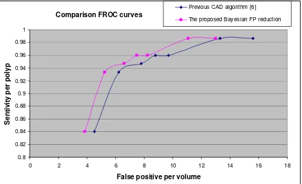
In our previous work, we have developed an entire automatic CT colonic polyp detection algorithm [6]. The aim of this experiment is to use the proposed Bayesian method to further remove false regions. For each candidate region, a polyp probability map based on Bayesian framework (Eq.1) is calculated, where, the intensity model is based on Eq.2 and K2 feature is used for the shape model. A hysteresis thresholding and 3D labeling are then applied on each probability map. If a candidate region contains a set of 3D connected voxels with high probabilities of “polypness”, the region is kept as a potential polyp region. Otherwise, the region is considered to be a non-polyp region and removed from the polyp candidates.
[image:6.595.125.472.134.265.2]
Comparison FROC curves
0.8 0.82 0.84 0.86 0.88 0.9 0.92 0.94 0.96 0.98 1
0 2 4 6 8 10 12 14 16 18
False positive per volume
S
e
n
ti
v
it
y
p
e
r
p
o
ly
p
Previous CAD algorithm [6]
[image:7.595.177.397.137.271.2]The proposed Bayesian FP reduction
Fig.4 FROC curves demonstrating the improvement of the Bayesian approach compared to our previous CAD algorithm.
4 Conclusion
We have presented a Bayesian approach to reduce false positives in CTC CAD. For each candidate region, the polyp likelihood is modeled using a combination of shape, and intensity features. The second principal curvature flow is used as a shape model; while PVE is considered into modeling the polyp intensity distribution. The proposed method has been applied on the candidate regions obtained from our previous CAD algorithm [6] on a multi-centre dataset of colonic CT, and it shows an average 16% reduction of FPs while keeping the same sensitivity. The method provides robust and consistent performance.
The Bayesian framework is general and can be flexibly extended to incorporate other features, Indeed, one could imagine incorporating other image features (location, texture) as well as patient informatics (age, family history of colorectal disease) for robust detection. The algorithm can also be easily adapted to candidate generation step of CAD system.
References
1. D.S.Paik, C.F.Beaulieu, G.D.Rubin, B.Acar, R.B.Jeffrey, J.Yee, J.Dey, and S.Napel, “Surface normal overlap: A computer-aided detection algorithm with application to colonic polyps and lung nodules in helical CT”, IEEE Trans. Medical Imaging, 23(6). (2004). 2. H.Yoshida, J.Nappi, “Three-dimensional computer-aided diagnosis scheme for detection of
colonic polyps”, IEEE Trans. Medical Imaging, 20, 1261-1274. (2001).
3. R.Summers, J.Yao, P.Pickhardt, M.Franaszek, I.Bitter, D.Brickman, J.R.Choi, “Computed tomographic virtual colonoscopy computer-aided polyp detection in a screening population”, Gastroenterology, 129, 1832-1844. (2005).
4. C.van Wijk, V.F.van Ravesteijn, F.M.Vos and L.J.van Vliet, “Detection and segmentation of colonic polyps on implicit isosurfaces by second principal curvature flow”, IEEE Trans. Medical Imaging, 29 (3). 688-698. (2010).
5. P.R.S.Mendonca, R.Bhotika, F.Zhao, J.Melonakos, and S.Sirohey, “Detection of polyps via shape and appearance modeling”, Proc MICCAI 2008 workshop: Computational and Visualization Challenges in the New Era of Virtual Colonoscopy. (2008).