City, University of London Institutional Repository
Citation
:
Salim, S. G. R., Fox, N. P., Hartree, W. S., Woolliams, E. R., Sun, T. & Grattan, K. T. V. (2011). Stray light correction for diode-array-based spectrometers using amonochromator. Applied Optics, 50(26), pp. 5130-5138. doi: 10.1364/AO.50.005130
This is the accepted version of the paper.
This version of the publication may differ from the final published
version.
Permanent repository link:
http://openaccess.city.ac.uk/14965/Link to published version
:
http://dx.doi.org/10.1364/AO.50.005130Copyright and reuse:
City Research Online aims to make research
outputs of City, University of London available to a wider audience.
Copyright and Moral Rights remain with the author(s) and/or copyright
holders. URLs from City Research Online may be freely distributed and
linked to.
City Research Online: http://openaccess.city.ac.uk/ [email protected]
Stray light correction for diode-array-based
spectrometers using a monochromator
Saber G. R. Salim,
1,2,3,* Nigel P. Fox,
2William S. Hartree,
2Emma R. Woolliams,
2Tong Sun,
3and Kenneth T. V. Grattan
31
National Institute of Standards (NIS), Tersa Street, El-Haram, P.O. Box 136, Giza 12211, Egypt
2National Physical Laboratory (NPL), Hampton Road, Teddington, Middlesex, TW11 0LW, UK
3City University London, Northampton Square, London, EC1V 0HB, UK
*Corresponding author: [email protected]
Photodiode-array-based spectrometersareincreasinglybeingusedinawidevarietyofapplications.
However,thesignalmeasuredbythistypeofinstrumentoftenisnotwhatisanticipatedbytheuser
andisoftensubjecttocontaminationfromstraylight.Thispaperdescribesanefficientandlow-coststray
lightcorrectionapproachbasedonarelativelysimplesystemusingamonochromator-basedsource.The
paperfurtherdiscussesthelimitationsofusingamonochromatorinsteadofalaser,asusedbyprevious
researchers,anditsimpactonthequalityofthestraylightcorrection.Thereliabilityandrobustnessofthe
straylightcorrectionmatrixgeneratedhavebeenstudiedandarealsoreported.
1. Introduction
A photodioarray-based spectrometer can be de-fined as a dispersive instrument with multiple opti-cal sensors that enables simultaneous acquisition of the radiant flux over a particular spectral range [1]. These instruments are in general characterized by their small size, light weight, and low cost. In addi-tion, they have the key advantage of capturing a spectrally resolved signal over a wide spectral range in a very short time compared to many mechanical scanning spectrometers. This has led to their wide-spread use in applications where signals are low, un-stable, or short lived. Diode array spectrometers are becoming the preferred tool for many applications using optical radiation, for example, in remote sens-ing, spectroscopy, astrophysics, analytical chemistry, health, and process control [2–5].
Although such spectrometers have many ad-vantages, they almost always suffer from stray light—arising from situations where the measured spectrally resolved signal is contaminated with ra-diation of a nominally different spectral content. A well-designed spectrometer, fitted with a high-quality diffraction medium (usually a grating), will minimize stray light, but it rarely will do so adequately. Further improvement can be obtained by using“cut-on”filters (usually glasses with a spectrally sharp transition be-tween high absorption and high transmittance, e.g., RG 665 glass from Schott) in front of the array detec-tor to remove higher order diffraction effects. How-ever, even in the best spectrometers, the stray light value measured at any pixel, obtained from a mono-chromatic source of a different wavelength, is of the order of10−5of the true in-band (IB) monochromatic
which has a significant impact on the final signal mea-sured. This issue can be an even greater problem for any part of the spectrum where the desired signal is relatively weak, e.g., the blue for an incandescent lamp as compared to the red, for example.
The responsivity of a diode array spectrometer is usually obtained by calibration against a reference standard source, such as a tungsten lamp of known spectral distribution. It is subsequently used to detect radiation from sources or surfaces with different spectral distributions, such as oceans, sky, and land surfaces and sources such as lasers or LEDs. Because of the spectral mismatch between the calibration source and the source under test, the stray light signal is not canceled out by a simple substitution process. This limits the accuracy and reliability of spectral measurements carried out using an array spec-trometer. It is thus essential that the stray light performance of such instruments is assessed prop-erly for each application, particularly for those requiring high accuracy and where necessary and possible, corrections for the presence of stray light are made.
2. Sources of Stray Light inside an Array Spectrometer
Ideally, each pixel in an array spectrometer should detect only the radiation with a spectral content characterized by those wavelengths directed to it by the dispersing element, without sensing any contri-bution from light at any other wavelengths. In prac-tice, there is always some response due to other wavelengths (i.e., what is termed “stray light”) that ideally should not be present but is. The major sources of stray light inside diode array spectro-meters can be summarized as follows:
i. Scattered light from the internal walls and input optics of the spectrometer.Light that deviates from the desired optical path and light from negative, zero and higher orders can be reflected onto the array detector from the internal walls or other components of the spectrometer.
ii. Dispersive element, usually a diffraction grating.Diffraction grating limitations are more ap-parent in photodiode array spectrometers than in mechanical scanning spectrometers: higher order diffraction signals “pollute” the desired first-order diffraction, and ruling imperfections in the grating grooves and coatings may lead to further scattering effects [6]. In addition, “cut-on” filters are used in front of the array elements to eliminate higher order diffraction signals, but these filters themselves be-come sources of stray light.
iii. Interreflections. Some light is always re-flected by each optical detector element onto other parts of the spectrometer. If cut-on filters are used, some of this reflected light will be rereflected back onto the sensor or its neighboring pixels. This is termed “near-field stray light” and appears as a
“hump” near the profile of a monochromatic light
source. This near-field signal can be quite significant, as observed by Zonget al. [7].
iv. Light coupling. Design constraints of the spectrometer, particularly related to the way that light is coupled into it, may also be a source of stray light. This may occur, for instance, when using a fiber with a larger numerical aperture (NA) than that spe-cified by the design increases stray light levels.
3. Existing Stray Light Correction Methods
Several approaches have been suggested to evaluate and correct for the spectral effects of stray light in diode array spectrometers. One such approach, proposed by Brown et al. in 2003 [1], depends on characterizing the slit scattering function (SSF) (pro-posed by Kostkowski [8]). The SSF is commonly used for stray light evaluation in mechanical scanning spectrometers, where the monochromator is held at a particular wavelength setting then illuminated by a series of monochromatic wavelengths.
Another more comprehensive (and relatively sim-ple approach) has been proposed by Zonget al. [7]. The method uses a spectrally tunable laser source to measure the full spectrometer response for differ-ent monochromatic input wavelengths. At each wavelength (λj), the spectrometer has a spectral line spread function (LSF) denoted byfLSF, which
repre-sents the response of each pixel to this wavelength. Because the incident light in such a case is mono-chromatic, any response at pixels outside the IB region, as detected by the spectrometer, can be con-sidered as stray light. This stray light signal can be evaluated by dividing the response at each pixeliby the integration of the IB signal after normalizing the value offLSF.
The resultant function is called the spectral stray light distribution function (di;j), and this can be
ex-pressed as [7]
di;j ¼
fLSF;i;j
P
i∈IB
fLSF;i;j; i∉
IB; ð1Þ
wheredi;j is the spectral stray light signal at pixeli
due to a monochromatic light that shows its maxi-mum at pixel j. An n×n stray light distribution matrix (D) can be formed by populating the matrix with the individual elements,di;j.
When light from a broadband source illuminates the photodiode array, the measured signal (Ymeas)
can be expressed as the sum of the signal for no stray light (YIB) plus the contribution of the stray light to
this signal:
Ymeas¼YIBþD·YIB¼ ½1þDYIB¼AYIB; ð2Þ
where A is called the square coefficient matrix. In such a case, the correction obtained by Zong et al.
[7] is given by
where C is called the stray light correction matrix, which is the inverse ofA.
In practice, the stray light distribution matrix (D) can be obtained from knowledge of a reasonable sub-set of the elements,di;j measured at different
wave-lengths across the spectral range of the spectrometer. The remainder of the n number of columns can be interpolated and, with care, extrapolated.
In the work carried out by Zonget al.[7], a tunable laser was used to determine the spectrometer response to a set of wavelengths across its range of operation to obtain the inputs for the matrixD.
The work carried out and reported in this paper has aimed to demonstrate how this approach could be further simplified through the use of monochro-mator-generated radiation.
4. Monochromator-Based Correction
Unlike spectrally tunable lasers, monochromators are widely available at relatively low cost and are easy to use. They are readily accessible, not only to national metrology institutes but also to commercial organizations. A monochromator-based approach has previously been implemented, as presented by Lenhard et al.[9], but this paper explores this con-cept in significantly more detail. While monochro-mators have a number of operational advantages, they also suffer from some issues that may limit the overall performance achievable, e.g., the source bandwidth, the output radiation levels, and the pre-sence of inherent stray light. There is an interrela-tionship between these factors; for example, output levels can be increased by using larger bandwidths but this, of course, compromises spectral resolution. This work reviews these limitations and their impact on the correction obtained.
A. System Bandpass Function
1. Calculating the System Response Function
When a laser source is used, the overall system bandpass function will be essentially that of the spec-trometer. For a monochromator-based method, the system bandpass function is given by a combination of the monochromator and spectrometer bandpass functions.
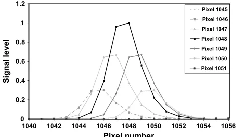
This interaction between the diode array spectro-meter and monochromator was studied using a sim-ple model that allowed an estimation of the shape of the overall system bandwidth and the signal level. The spectrometer bandpass function was taken to be that measured using an He–Ne laser at 632:8nm, and the monochromator bandpass function was as-sumed to be a triangular function of 1nm FWHM. The bandpass functions of the spectrometer and monochromator were normalized to unity at their maxima, as shown in Fig. 1.
Each point on the monochromator bandpass func-tion was assumed to result in the same spectrometer bandpass profile as if it were a laser, i.e., being
equivalent to the output of the He–Ne laser, as shown in Fig. 2.
The spectrometer signal at a particular pixel is thus the sum of the pixel responses to each point on the monochromator bandpass function. The dark-est (black) line in Fig.3shows the combination of the monochromator and the spectrometer bandpasses, as calculated by the model. The calculated resultant system bandpass (∼1:6nm FWHM) is slightly wider than the spectrometer bandpass function obtained using the laser (∼1:2nm FWHM) and the monochro-mator bandpass profile (∼1nm FWHM).
It should be noted that this approach can be created by convolving the monochromator spectrom-eter bandpass function xðnÞ and the spectrometer bandpass function, as described elsewhere in the lit-erature [10]. The convolution YðnÞ can simply be written as
YðnÞ ¼xðnÞ yðnÞ ¼ X
n
i¼−n
xðiÞyðn−iÞ; ð4Þ
wherenis the pixel number andiis an integer in this case. This equation is numerically intensive to eval-uate; therefore, it can be converted into a multiplica-tion by using a FFT such as
0.00 0.25 0.50 0.75 1.00 1.25
1040 1042 1044 1046 1048 1050 1052 1054 1056
Pixel number
Signal le
vel,
normaliz
ed
[image:4.594.308.543.555.692.2]Spectrometer bandpass function Monochromator bandpass function
Fig. 1. Spectrometer bandpass and the monochromator bandpass functions—theX axis is replaced by the pixel order inside the array detector rather than the wavelength.
Y¼IFFTðFFTðxÞFFTðyÞÞ: ð5Þ
Although this approach is straightforward, it may be necessary to apply windows (e.g., Hanning) to the functions, which may affect the profile of the band-width in the final result. In addition, it may be re-quired to remesh the functions so they are on the same grid.
The applicability of the model was confirmed ex-perimentally by measuring the bandpass function of the instrument using the system shown in Fig.4. The measured bandpass profile was found to be very close to that calculated by the model (the dark gray line shown in Fig.3).
Even with wider monochromator bandpass values (of 2 and 3nm—these are wider than the spectro-meter bandpass), the system bandpass was found to be only slightly larger than the monochromator bandpass. However, the best results were obtained experimentally with the slit width of the monochro-mator set to be as narrow as possible, to make the system bandwidth and spectrometer bandwidth very close to each other in value—although there will be a compromise in this choice when the signal levels are small.
2. Bandpass Profile and Stray Light Calculations
The chosen width of the“IB”region affects the resul-tant stray light correction matrix, as the spectro-meter response at each pixel element is divided by the integration over the IB region. The width of
the IB region increases at higher wavelengths due to the increased bandwidth of the spectrometer, also the level of the near-field stray light has been found to vary across the spectrometer spectral range. Therefore, it is seen as important to take these con-siderations into account when defining the IB region, and this was done.
B. Stray Light Signal inside the Monochromator
Unlike a laser, monochromators will have their own stray light. Therefore, the stray light correction should be carried out using a double grating mono-chromator in which the associated internal stray light is typically of the order of∼10−6. Ideally, the
re-sidual stray light should be completely prevented from entering the spectrometer, but this is not easily achieved in practice. However, the effect of this small level of monochromator-based stray light is thought to be negligible in the operation of the system.
5. Experiment and Setup
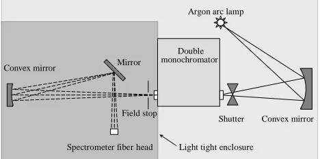
The experimental system used in this work, shown in Fig.4and based largely on the NPL spectral respon-sivity facility, was set up to conduct the stray light correction. An argon arc lamp, which has a relatively high spectral emission (especially in the UV region), was used. The light emitted from the lamp was fo-cused onto the entrance slit of a double monochroma-tor using a convex mirror.
The monochromator output light was directed by convex and plane mirrors to the lens attached to the SMA connection of the spectrometer fiber. This lens is used to define the field of view of the spectrometer. The f number of the beam could be adjusted using a field stop located beyond the exit slit of the mono-chromator. During the measurements carried out, care was taken to ensure that the light overfilled the lens aperture to mimic normal operation. The spec-trometer fiber lens was aligned to maximize the collection of light; this occurred when the spot (repre-senting the optical beam) on the plane mirror was located in the field of view of the fiber lens.
Higher order diffraction was suppressed during the spectral scan of the monochromator by the use of cut-on filters inside the monochromator facility, operating at wavelengths of 390 and 670nm. This in turn ensured a further reduction of the stray light inside the monochromator.
Below a wavelength of 650nm, gratings with a blaze of 500nm were used, while for longer wave-lengths, gratings with a blaze of 700nm were employed in this work. The lamp current was opti-mized to ensure that a reasonable signal level was obtained over all the spectral regions studied.
The spectrometer used for the tests carried out is a commercial instrument that employs a high-sensitivity miniphotodiode array manufactured by Hamamatsu (type C10083CAH), and the array de-tector is a 2048 pixel element back-thinned silicon photodiode array. The spectrometer covers the spec-tral range from 208 to1078nm; as this also covers
0.00 0.25 0.50 0.75 1.00 1.25
628 629 630 631 632 633 634 635 636 637 638 Wavelength /nm
Signal le
vel,
normaliz
ed
Spectrometer bandpass profile using laser Expected profile using the model
[image:5.594.52.286.583.699.2]Measured profile using monochromator system
Fig. 3. Convolution of the spectrometer and the monochromator bandpass functions: model and experimental results.
Argon arc lamp
Double monochromator
Convex mirror Mirror
Field stop
Spectrometer fiber head Convex mirror
Shutter
Light tight enclosure
most of the silicon detector responsivity range, errors due to stray light from wavelengths outside this range were considered negligible. The analog-to-digital converter used with the spectrometer has 16bit resolution, which means that one single count is 1:52×10−5 of the maximum number of counts
(65,536). To detect stray light values less than this level, the spectrometer output signal was sampled 1000 times, ensuring sufficient resolution in the stray light measurement (i.e., a signal level could be obtained to sufficient significant figures) to eval-uate the actual low-level stray light present.
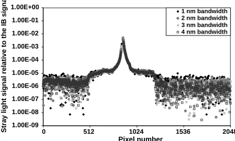
To study the impact of the monochromator band-width on the efficiency of the stray light correction matrix, the column vector di;j was evaluated by the
measurements at 555nm, for four different mono-chromator bandwidths (1, 2, 3, and 4nm), and the results obtained are shown in Fig.5.
For the bulk of the spectrum, it can be seen that the results obtained are nearly identical. However, the use of narrower bandwidths is required to deter-mine the stray light levels at the pixels immediately adjacent to the IB region. This means that to obtain a measurable signal, priority should be given to either increasing the source signal or using a higher in-tegration time, rather than simply using a wider monochromator bandwidth. The monochromator slit width was therefore adjusted to give a 1nm band-width, and the lamp power increased to ensure a rea-sonable signal-to-noise ratio was obtained. The same bandwidth was used over the entire wavelength do-main to ensure consistent results for the values given by di;j.
The nonlinearity performance of the spectrometer has been found to be affected by using different inte-gration times and different source intensities [11]. The impact of these two factors on the values of the spectral stray light distribution function has been studied. The effect of using different integration times was studied at a wavelength of850nm, where integration times of 10, 20, and30ms were used to tune the spectrometer signal level from a maximum of 20,000 counts to nearly 60,000 counts, while keep-ing a fixed source intensity. No noticeable differences in the resultant values of di;j were observed, other
than obtaining improved noise characteristics for the use of higher integration times. The effect of using different source intensities was studied at a wave-length of 550nm, while keeping a fixed integration time. The results of this effect are shown in Fig. 6. The measured stray light was observed to increase slightly when low signal levels were used, but there was no noticeable change between the stray light level observed at signal levels of 40,000 and 60,000 counts. This can be explained in terms of the relative response of each pixel, which is slightly higher at lo-wer signal levels. The effect is generally small, but to ensure consistency, all subsequent analysis was done with signal levels greater than 20,000 counts.
6. Results
A. Spectral Stray Light Distribution Function
The spectrometer signal was measured at5nm inter-vals over the whole spectral range. At each measured wavelength, a corresponding dark signal was also re-corded. The dark-corrected spectrometer signal was normalized to the maximum level to obtain the value of fLSF. Although all the spectral LSFs were
mea-sured at high integration times, some pixels gave ne-gative values as a result of noise in the dark and light signals. However, the number of such pixels was, in general, small, as were the values of the (negative) numbers they gave. The values offLSFhave been
cal-culated as a result of repeated measurements at a wavelength of550nm, following which the results ob-tained were compared. It was noticed that when the experiment was repeated, these negative values were not repeatable for these specific pixels, thereby confirming that these results were simply due to noise. Ideally, noise with both signs (negative and positive) should be removed from the “real”signal; however, it is not possible to distinguish noise with a positive sign from the stray light signal. Therefore, it was decided in the analysis to replace any negative values obtained with a zero, as they did not represent a real stray light signal. Further justification for this was that, in addition, leaving the negative val-ues may result in “undercorrecting” the stray light
1.00E-09 1.00E-08 1.00E-07 1.00E-06 1.00E-05 1.00E-04 1.00E-03 1.00E-02 1.00E-01 1.00E+00
0 512 1024 1536 2048
Pixel number
Stra
y light signal relative to the IB signal
[image:6.594.311.541.41.180.2]1 nm bandwidth 2 nm bandwidth 3 nm bandwidth 4 nm bandwidth
Fig. 5. Spectral stray light distribution function for different monochromator bandwidths. 1.0E-09 1.0E-08 1.0E-07 1.0E-06 1.0E-05 1.0E-04 1.0E-03 1.0E-02 1.0E-01 1.0E+00
0 512 1024 1536 2048
Pixel order l a n gi s BI e ht ot e vi t al er l a n gi s t h gil y ar t S
[image:6.594.52.283.554.693.2]60,000 40,000 20,000 10,000
signal. It is important to note that a“rolling average” signal to reduce noise should be avoided, as this was found to result in poorer correction than the approach suggested.
The IB region was determined manually by care-fully selecting the pixels defining the“wings”before integration. The spectrometer signal at each pixel was then divided by the integral of the IB signal to obtain the values ofdi;j required.
The values offLSF obtained showed no signal for
input wavelengths below 270nm despite a signifi-cant output from the monochromator (as measured by a reference photodiode). This lack of a spectro-meter response was attributed to the very poor trans-mittance of the lens in this region. As a consequence, zero values forfLSFwere used in the spectral range
below270nm.
With input wavelengths from 270 to340nm, there was some noticeable second-order diffraction light, as shown bydi;j and illustrated by the black line in
Fig. 7. This second-order diffraction was not visible for longer wavelengths. The stray light levels were also higher for wavelengths corresponding to pixels located at both ends of the spectrometer detector array than for those pixels in the middle.
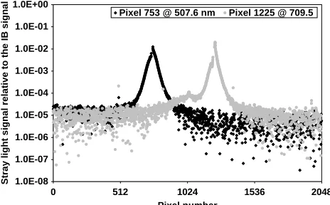
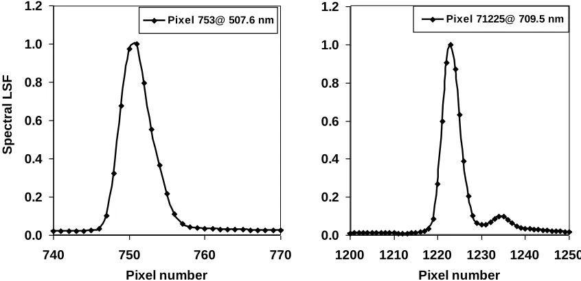
By comparison to Fig.7, Fig.8shows an increased IB width at wavelengths around 500 and700nm due to an increase in the near-field stray light signal. A finer scanning of the input wavelength, at1nm inter-vals, was used to examine thoroughly the stray light levels in these regions. Figure9shows the values ob-tained for fLSF for inputs at wavelengths of around
507.6 and709:5nm (corresponding to pixel numbers 753 and 1225), which represent the observed center of this increased IB width.
According to the manufacturer’s literature, there are three cut-on filters, which are used to block the higher order diffraction signals (these are types WG305, GG475, and RG665). The boundaries be-tween the filters occur at pixels that correspond to wavelengths of 507.6 and 709:5nm. This is likely to result in an increase in the scattered light in the region of these pixels and hence the broadening in the stray light profile. The presence of these filters also explains the reduced signal level in the vicinity
of these wavelengths when the spectrometer is ex-posed to light from a broadband source.
Because of this, the spectral ranges around 507 and 709nm were measured at input spectral inter-vals of1nm so as to show the exact spectral distribu-tion of the stray light around those pixels.
B. Stray Light Correction Matrix
The stray light correction algorithm used is required to ensure that it not only provides a good estimate of stray light but also that it does not alter any other characteristic of the spectrometer under test. For example, a poor correction matrix may lead to a de-crease in the apparent signal-to-noise level of the spectrometer. To test the reliability of the stray light correction matrix, measurements of two stray light sensitive sources were analyzed, while modeling was also performed to understand the sensitivity to noise.
1. Performance of the Stray Light Correction Matrix
Having calculateddi;j at the pixels where
measure-ments were made, values for di;j in other regions
were interpolated using a MATLAB routine within the stray light correction software [12]. To deliver an accurate near-field correction, di;j was
interpo-lated along the matrix diagonals (parallel to the matrix main diagonal).
The stray light distribution matrix is shown in Fig.10. The figure further shows an increased near-field stray light signal in the IR region. The second-order diffraction stray light is also shown in the figure at the shorter wavelengths.
The effectiveness of the stray light correction matrix to achieve a suitable correction for the stray light was tested using two sources: a low argon pressure lamp and a tungsten halogen lamp, with the output filtered with a 630nm cut-on filter. In each case, the measured signal was normalized to the maximum before the stray light correction was applied. 1.0E-09 1.0E-08 1.0E-07 1.0E-06 1.0E-05 1.0E-04 1.0E-03 1.0E-02 1.0E-01 1.0E+00
0 512 1024 1536 2048 Pixel number l a n gi s BI e ht ot e vit al er l a n gi s t h gil y ar t S
Pixel 166 @ 270 nm Pixel 491@ 400 nm Pixel 971@ 600 nm Pixel 1430 @ 800 nm Pixel 2048 @ 1078.7 nm
Fig. 7. Spectral stray light distribution function (di;j) at different input wavelengths. 1.0E-08 1.0E-07 1.0E-06 1.0E-05 1.0E-04 1.0E-03 1.0E-02 1.0E-01 1.0E+00
0 512 1024 1536 2048 Pixel number l a n gi s BI e ht ot e vi t al er l a n gi s t h gil y ar t S
[image:7.594.310.542.37.181.2]Pixel 753 @ 507.6 nm Pixel 1225 @ 709.5
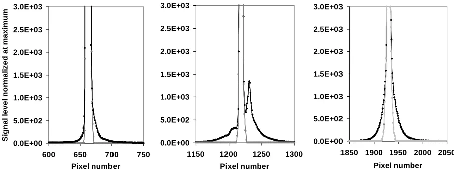
[image:7.594.52.285.561.692.2]The cut-on filter signals before and after correction was applied are shown in Fig.11for the filtered lamp and Fig.12for the spectral lines of the argon lamp. Figure11shows a signal level<10−6below the filter
cut-on wavelength and a reduced signal level in the IR region where stray light also would be expected. Figure 12 shows the use of the correction has re-sulted in a nearly ideal shape of the spectral profile of the selected argon lines. In addition, the stray light in the far field has also been reduced by nearly 1 order of magnitude.
Having obtained these high-quality results, the reliability of the correction matrix when using a smaller number of input data points was evaluated. In this example, the resolution of the scanning of the input wavelength was reduced to 20nm inter-vals, contrasting with the 5nm interval previously used. For the highly sensitive regions at wavelengths around 507 and 709nm, data taken every 3nm (contrasting with the previous 1nm) were used. The new stray light correction matrix showed iden-tical results to those obtained previously with the whole set of measured points. Thus, relatively few
characterization wavelengths are required for the determination of an accurate stray light correction matrix; however, where there are anomalies, e.g., where cut-on filters may overlap, it is clear that a more detailed spectral evaluation is required.
2. Matrix Sensitivity Coefficient
For a linear algebraic system, such as that repre-sented by Eq. (2), the sensitivity of the solution (YIB)
to changes in the measured signal given by the spec-trometer (Ymeas) and the square coefficient matrix (A)
can be studied using the condition number of the square coefficient matrixA[13]. The condition num-ber is defined as the product of the norm ofAand the norm ofA−1. This number is always greater than or
[image:8.594.79.502.36.241.2]equal to 1. If it is close to 1, this means that the ma-trix inverse can be calculated with high accuracy; however, if it is much larger, this means that the ma-trix inverse is“ill-conditioned”and cannot be calcu-lated accurately. A large condition number will mean the correction is more sensitive to measurement errors in the determination of the stray light cor-rection matrix, and less able to reproduce small
Fig. 10. 3D stray light distribution matrix obtained by using di-agonal interpolation.
1.0E-07 1.0E-06 1.0E-05 1.0E-04 1.0E-03 1.0E-02 1.0E-01 1.0E+00
0 512 1024 1536 2048 Pixel number
n
oi
t
c
er
r
o
c
er
of
e
b
d
n
a
r
et
f
a l
a
n
gi
s
r
etl
i
F
Filter signal before correction
[image:8.594.51.285.555.693.2]Filter signal after correction
Fig. 11. Cut-on filter signal before and after stray light correc-tion.
0.0 0.2 0.4 0.6 0.8 1.0 1.2
740 750 760 770
Pixel number
Spectral LSF
Pixel 753@ 507.6 nm
0.0 0.2 0.4 0.6 0.8 1.0 1.2
1200 1210 1220 1230 1240 1250
Pixel number
Pixel 71225@ 709.5 nm
[image:8.594.308.540.559.692.2]variations in the spectrum being recovered. A condi-tion number equal to infinity means that the matrix is noninvertible.
For the correction of the spectrometer used in this work, the condition number of the square coefficient number was found to be 1.86, which is somewhat higher than the value 1.07 obtained by Zong et al.
[7]. This is likely mainly to be due to the fact that this stray light correction matrix was zero for input wavelengths below270nm (due to the lens transmit-tance), and, in addition, the signal also had relatively high stray light signals at longer wavelengths.
As the condition number was somewhat higher, it was considered necessary to check the sensitivity of YIBto variations inYmeas. A spectral structure of
per-iodically oscillating amplitude of0:5%of the value ofYmeas was deliberately added toYmeas for a
tung-sten lamp signal, andYIBwas calculated before and
after adding this periodic oscillation. The difference between the two output spectra showed the same periodic spectral structure with a corresponding os-cillating amplitude of 0:56% at 400nm increasing gradually to0:72%at1078nm. In addition, random noise of relative amplitude within0:5%was added to Ymeas, and YIB was recalculated before and after
adding this random noise. The difference between the two output spectra was found to be similar to the values observed when adding the periodic oscillation toYmeas. These tests show that the stray light
correc-tion matrix causes only minor distorcorrec-tions to small changes in the spectrum being measured, and the condition number for this spectrometer is acceptable.
7. Summary
This paper has shown that one of the major sources of uncertainty that limits the performance of the diode-array-based spectrometers—stray light—can be ac-curately corrected with a relatively fast procedure using cheap and readily available monochromators, with results comparable to those obtained using tunable lasers. The work reported in this paper has described the sensitivity of the stray light character-ization method to both the measurement system and
subsequent mathematical evaluation processes. It also has shown that the number of measurement points needed for the correction can be reduced signif-icantly without impacting on the overall performance of the system.
The application of these procedures could be used to make it possible for low-cost spectrometers of this nature to move from being useful spectral monitoring devices to high-performance optical spectroradiom-eters capable of transforming optical radiation mea-surement in a wide variety of applications that currently are limited by the achievable accuracy or by the lack of flexibility arising due to large immova-ble instrumentation.
The authors would like to acknowledge the contri-bution of Ian Smith of the NPL Scientific Computing Team for his help in writing the MATLAB code for diagonal interpolation and Andrew Levick for his valuable comments. One of the authors (S. Salim) gratefully acknowledges the award of a fellowship from the Cultural Affairs & Scientific Missions Sec-tor, Egypt. This work was supported by the National Measurement Office of the UK Department “ Busi-ness, Innovations, and Skills (BIS).”
References
1. S. B. Brown, B. C. Johnson, M. E. Feinholz, M. A. Yarbrough, S. J. Flora, K. R. Lykke, and D. K. Clark,“Stray-light correction algorithm for spectrographs,”Metrologia40, S81–S84 (2003). 2. M. Belluso, M. C. Mazzillo, S. Billotta, S. Scuderi, A. Calí, A. Micciché, M. C. Timpanaro, D. Sanfilippo, P. G. Fallica, E. Sciacca, S. Lombardo, and A. Morabito,“SPAD array detec-tors for astrophysical applications,”Mem. S. A. It. Suppl.9, 430–432 (2006).
3. S. G. R. Salim, N. P. Fox, E. R. Woolliams, R. Winkler, H. M. Pegrum, T. Sun, and K. T. V. Grattan,“Use of eutectic fixed points to characterize a spectrometer for earth observations,” Int. J. Thermophys.28, 2041–2048 (2007).
4. H. Shen, T. J. Cardwell, and R. W. Cattrall,“The application of a chemical sensor array detector in ion chromatography for the determination of Naþ, NH4þ, Kþ, Mg2þ and Ca2þ in water samples,”Analyst123, 2181–2184 (1998).
0.0E+00 5.0E+02 1.0E+03 1.5E+03 2.0E+03 2.5E+03 3.0E+03
600 650 700 750
Pixel number
Si
gnal
l
e
vel
nor
m
al
iz
ed at
m
axi
m
u
m
0.0E+00 5.0E+02 1.0E+03 1.5E+03 2.0E+03 2.5E+03 3.0E+03
1150 1200 1250 1300
Pixel number
0.0E+00 5.0E+02 1.0E+03 1.5E+03 2.0E+03 2.5E+03 3.0E+03
1850 1900 1950 2000 2050
[image:9.594.70.522.34.203.2]Pixel number
5. S. S. Vogt, R. G. Tull, and P. Kelton,“Self-scanned photodiode array: high performance operation in high dispersion astro-nomical spectrophotometry,”Appl. Opt.17, 574–592 (1978). 6. C. Palmer, Diffraction Grating Handbook (Thermo RGL,
2002).
7. Y. Zong, S. B. Brown, B. C. Johnson, K. R. Lykke, and Y. Ohno, “Simple spectral stray light correction method for array spec-troradiometers,”Appl. Opt.45, 1111–1119 (2006).
8. H. J. Kostkowski,Reliable Spectroradiometry (Spectroradio-metry Consulting, 1997).
9. K. Lenhard, P. Gege, and M. Damm,“Implementation of algo-rithmic correction of stray light in a pushbroom hyperspectral sensor,”in6th EARSeL Imaging Spectroscopy SIG Workshop
(EARSeL, 2009), http://www.earsel6th.tau.ac.il/~earsel6/CD/ PDF/earsel‑PROCEEDINGS/3035%20Lenhard.pdf.
10. N. Ronald, Bracewell, The Fourier Transform and Its Applications(McGraw-Hill Science Engineering, 1999). 11. S. G. R. Salim, N. P. Fox, E. Theocharous, S. Tong, and K. T. V.
Grattan, “Temperature and nonlinearity corrections for a photodiode array spectrometer used in the field,”Appl. Opt.
50, 866–875 (2011).
12. MATLAB version 6.5.1. Natick, Mass., The MathWorks, Inc. (2003).