ASSESSMENT ON THE FEASIBILITY OF FUTURE SHEPHERDING OF ASTEROID RESOURCES J.P. Sanchez
Advanced Space Concepts Laboratory, University of Strathclyde, UK C.R. McInnes
Advanced Space Concepts Laboratory, University of Strathclyde, UK Most plausible futures for space exploration and exploitation require a large mass in Earth orbit. Delivering this mass requires overcoming the Earth’s natural gravity well, which imposes a distinct obstacle to any future space venture. An alternative solution is to search for more accessible resources elsewhere. In particular, this paper examines the possibility of future utilisation of near Earth asteroid resources. The accessibility of asteroid material can be estimated by analysing the volume of Keplerian orbital element space from which Earth can be reached under a certain energy threshold and then by mapping this analysis onto an existing statistical near Earth objects (NEO) model. Earth is reached through orbital transfers defined by a series of impulsive manoeuvres and computed using the patched-conic approximation. The NEO model allows an estimation of the probability of finding an object that could be transferred with a given ∆v budget. For the first time, a resource map provides a realistic assessment of the mass of material resources in near Earth space as a function of energy investment. The results show that there is a considerable mass of resources that can be accessed and exploited at relatively low levels of energy. More importantly, asteroid resources can be accessed with an entire spectrum of levels of energy, unlike other more massive bodies such as the Earth or Moon, which require a minimum energy threshold implicit in their gravity well. With this resource map, the total change of velocity required to capture an asteroid, or transfer its resources to Earth, can be estimated as a function of object size. Thus, realistic examples of asteroid resource utilisation can be
provided.
Keywords: Asteroid Exploitation; Asteroid Mining; Space Utilization; near-Earth Objects; Near-Earth Asteroids.
1. INTRODUTION
Any envisioned future for space exploration involves both a growth in large space structures and human presence in space. Some possible examples are space solar power, space tourism or more visionary human space settlements. This, of course, implies a much larger mass of material in-use in space, for both structural mass and life support. The traditional approach to deliver material into orbit has always been overcoming the Earth’s gravity well, which is, arguably, not the most effective means if we bear in mind, for instance, that the energy cost to reach low Earth orbit (LEO) is already “half-way to anywhere”*
Asteroids and comets, and more particularly, near-Earth Objects (NEOs), have long been recognised as possible alternative sources of material in space, and have been targets of speculative science on future space exploitation [
.
1, 2]. These small celestial bodies have been identified as possible reservoirs of useful materials such as water, metals and semiconductors. Asteroids are also of strategic importance in uncovering the formation, evolution and
composition of the solar system and, in particular, NEOs have risen in prominence because they are among the easiest celestial bodies to reach from the Earth and they may represent a long-term planetary threat [3]. The growing interest in these objects has translated into an increasing number of missions to NEOs, such as the sample return
missions Hayabusa[4] and Marco Polo[5], impactor missions such as Deep Impact† and possible deflector demonstrator missions such as Don Quixote‡
With regard to asteroid impact hazard and its mitigation, a range of methods have been identified as able to provide a change in the asteroid linear momentum [
.
6]. Some of these methods, such as the kinetic impactor or the low-thrust propulsion tugboat, may be argued to require shorter technology development than other more complex means to alter the momentum of the asteroid, such as the solar collector, simply because they are based on technologies that have been flown before. Thus, it is not inconceivable to think that methods such as the kinetic impactor or the low-thrust tugboat may become the first available technologies to produce small changes to the orbits of asteroids. Assuming then that some of these deflection technologies may be available in future, not only Earth-threatening objects could be nudged away from their collision trajectories, but also resource-rich asteroids may potentially be manoeuvred and captured into a bound Earth orbit through judicious use of orbital dynamics. Even if direct transfer of the entire NEO is not possible, or necessary, at least extracted resources could still be transferred to a bound Earth orbit for utilisation.
The main advantage of asteroid resources is that the gravity well from which materials would be extracted is much weaker than that of the Earth or the Moon. Thus, these resources could in principle be placed in a weakly-bound Earth orbit for a lower energy cost than material delivered from the surface of the Earth or Moon. A myriad of different materials could then be transported and utilised in space. Water and other volatiles, for example, could potentially be extracted from hydrated carbonaceous asteroids and be utilised for life support and propellant [7]. Humans need approximately 3 litres of water daily. Even if a significant fraction of this water is recycled, current water recycling systems require periodic resupply. Water and other volatiles could also be used as a rocket propellant. The possibility of stationing orbital refuelling depots, for example at the Lagrangian L2 point, to fuel
The question that arises then is how much near-Earth asteroid material is there which can be captured with a modest investment of energy. Modest investment refers here to an energy cost much lower than that required to transport resources from Earth or the Moon. The answer to this question may provide some insight on the general feasibility of asteroid exploitation and mining concepts. The paper will then attempt to answer this by analysing the volume of Keplerian orbital element space from which Earth can be reached under a certain limit of orbital transfer energy, and then mapping this analysis to the near Earth asteroid population. The resulting resource map provides an accurate assessment of the amount of material resources of near Earth space to be expected as a function of energy investment.
The population of near-Earth objects, described in Section 2, is modelled in this paper by means of an object size distribution together with an orbital element distribution function. The size distribution is defined via a power law relationship between the asteroid diameter and the total number of asteroids with size lower than this diameter [8]. On the other hand, the orbital distribution used in this paper will rely on the Bottke et al.[9] asteroid model to estimate the asteroid density to be expected in a given region of the Keplerian elements space.
The dynamical model used to study the Keplerian semi-major axis a, eccentricity e, inclination i orbital element space {a,e,i} of asteroid-to-Earth transfers assumes a circular Earth orbit with a 1 AU semi-major axis. The Sun is the central body for the motion of the asteroid, and the Earth’s gravity is only considered when the asteroid motion is in close proximity. Since the orbital transfers will be modelled as a series of impulsive changes of velocity, for some conditions, analytical formulae relate the total change of velocity with the region of Keplerian space that can be reached.
Two different transfer models are included in this paper, and described in Section 3. Firstly, a phase-free two-impulse transfer, which is composed of a change of plane manoeuvre and a perigee capture manoeuvre at Earth encounter. This transfer, as with a Hohmann transfer analysis, provides a good conservative estimate of the exploitable asteroid material. Secondly, a phase-free one-impulse transfer, which only considers a perigee capture manoeuvre during the Earth fly-by. In this second case, only orbits that have initially very low Minimum Orbital Intersection Distances (MOID) can be captured. The MOID is the minimum possible distance between the Earth and the asteroid considering free-phasing for both objects. Finally, an estimation of the phasing manoeuvre required to meet the Earth at the orbital intersections will also be included on the transfer sequence.
Section 4 will examine the accessibility of asteroids by analysing the statistical average size of the thousand first largest objects expected to be found within a given ∆v transfer to Earth. Section 4, as well as previous sections, will make no distinction among the different classes of asteroids or their resources. Section 5, instead, will provide a short discussion on the implications for some key resources on the results of asteroid accessibility.
2.
By convention, a celestial body is considered a Near Earth Object if its perihelion is smaller than 1.3 AU and its aphelion is larger than 0.983 AU. This is a very broad definition which includes predominantly asteroids, but also a small percentage of comets. NEOs are then the closest celestial objects to the Earth and therefore the obvious first targets for any resource exploitation mission (excluding the Moon).
The first NEA (Near-Earth Asteroid) was discovered in 1898 (433 Eros) and since then more than 7000 asteroids have been added to the NEO catalogue. Most of these objects have been surveyed during the last 20 years as a consequence of the general recognition of the impact threat that these objects pose to Earth [10]. This recognition led to a series of efforts to catalogue 90% of objects with the potential to pose a global environmental threat [11] (i.e., Diameter>1km). Subsequent recommendations suggested to pursue 90% completeness of the census of 140-m objects by 2020 [8]. The new generation of surveys such as LSST [12] or Pan-STARRS [13] are well positioned to achieve this objective.
Together with the ever-growing catalogue of asteroids, the understanding of the origin and evolution of these objects has seen enormous advancements in recent years [14]. Still, it is not possible to know accurately the amount and characteristics of asteroid exploitable resources. However, reliable order of magnitude estimates may now provide some insight concerning the feasibility of future space resource exploitation and utilisation concepts (e.g., space-based climate engineering[15]).
In order to determine near-Earth resource availability, a sound statistical model of the near Earth asteroid population is required. The following sections will describe an asteroid model of the fidelity necessary to allow the order of magnitude analysis. The asteroid model described is composed of two parts; a size population model, which describes the net number of asteroids as a function of object size and an orbit distribution model that describes the likelihood that an asteroid will be found in a given region of orbital element space.
2.1
The NEO size distribution is taken from the Near-Earth Object Science Definition report[Near Earth Object Population 8]. It is based on the results of a substantial number of studies estimating the population of different ranges of object sizes by a number of techniques (see Fig. 1 taken from Stokes et al. [8]). The Near-Earth Object Science Definition report provides an accumulative population of asteroids that can be expressed as a constant power law distribution function of object diameter as:
( [ ]) b
N >D km =CD−
(1)
Fig. 1: Accumulative size distribution of Near Earth Objects (from Stokes et al. [8]).
Assuming a population of asteroids defined by a power law distribution such as Eq.(1), one can easily calculate the total number of objects within an upper and lower diameter range:
(
min max)
(
min b max b)
N D D D C D − D −
∆ < ≤ = − (2)
where Dmax and Dmin are the maximum and minimum diameter chosen. An estimation of the total asteroid mass
composed by all these objects can also be computed. To do so, the following integration needs to be performed:
(
)
min
max min max
[ ] [ ]
D
D
N
N
D D D km
M
−=
∫
m dN
⋅
>
(3)
where m is the mass of the asteroid and
N
DminandN
Dmaxare the number of objects bigger than Dmin and Dmax respectively.Assuming that all asteroids have a spherical shape and an average density
ρ
a, the mass m of the asteroid can bedefined by
( )
π
6
⋅ ⋅
ρ
aD
3 and the integration can be defined as an integration over the asteroid diameter:min
max min max
3
[ ] 6 a
D
D D
D
dN
D dD
dD
M
−=
∫
π
⋅ ⋅ρ
⋅
(4)
where dN dD is the derivative of Eq.(1) with respect the diameter D. Integrating Eq.(4), the total mass of asteroid material composed of asteroids with diameters between Dmax and Dmin results in:
max min
3 3
max min
[ ] 6 3
b b
a
D D C b D bD
M
− π ρ⋅ ⋅ ⋅ − −− −
=
(5)
The average asteroid density
ρ
acan be approximated as 2600 kg/m3 (ref.[16]). Thus, for example, Eq.(5) canyield the total mass of “Tunguska” size objects (i.e., from 50 m to 70 m diameter) in near Earth space as being in the order of 1014 kg[17]. More recent estimates of the population of small asteroids [11] seem to indicate a possible drop
Finally, if the maximum diameter is set equal to the largest near Earth object known, 1036 Ganymed, which is 32 km in diameter and the minimum object size is set at 1 meters diameter, then Eq. (5) yields a total mass of 4.38x10¹⁶
kg. Note that the mass of a 32-km diameter spherical object with a density of 2600 kg/m3 is already higher than the
estimation yielded by Eq.(5). The reason for this is that the power law distribution (1) underestimates the number of large objects existing. Nevertheless, this result will be taken as the estimated total mass of asteroid material available in near Earth orbit space. Now, it is necessary to define the energy requirements for transporting this material to Earth orbit in order to draw conclusions concerning practical resource availability.
2.2
This section describes the NEO orbital distribution model used to estimate the likelihood of finding an asteroid within a given volume of Keplerian orbital element space
Near Earth Object Orbital Distribution
{
∆ ∆ ∆ ∆Ω ∆ ∆
a e i
, , ,
,
ω
,
M
}
. This likelihood can also beinterpreted as the fraction of asteroids within the specified region of the Keplerian space, and thus, if multiplied by Eq.(5), results in the portion of asteroid mass within that region. Hence, the ability to calculate this likelihood, together with the ability to define the regions of the Keplerian space from which the Earth can be reached with a given ∆v budget, will later allow us to compute the asteroid resources available in near-Earth space.
The NEO orbital distribution used here is based on an interpolation from the theoretical distribution model published in Bottke et al.[9]. The data used was very kindly provided by W.F. Bottke (personal communication, 2009). Bottke et al.[9] built an orbital distribution of NEOs by propagating in time thousands of test bodies initially located at all the main source regions of asteroids (i.e., the ν6 resonance, intermediate source Mars-crossers, the 3:1 resonance, the outer main belt, and the trans-Neptunian disk). By using the set of asteroids discovered by
Spacewatch at that time, the relative importance of the different asteroid sources could be best-fitted. This procedure yielded a steady state population of near Earth objects from which an orbital distribution as a function of semi-major axis a, eccentricity e and inclination i can be interpolated numerically.
The remaining three Keplerian elements, the right ascension of the ascending node Ω, the argument of periapsis ω and the mean anomaly M, are assumed here to be uniformly distributed random variables. The ascending node Ω and the argument of periapsis ω are generally believed to be uniformly distributed in near Earth orbit space [18] as a consequence of the fact that the period of the secular evolution of these two angles is expected to be much shorter than the life-span of a near Earth object [19]. Therefore, we can assume that any value of Ω and ω is equally possible for any NEO. All values of mean anomaly M are also assumed to be equally possible, and thus M is also uniformly distributed between 0 to 2π.
Fig. 2: Theoretical Bottke et al. [9] NEO distribution. The figure shows the integrated projections of the function
ρ(a,e,i) and a set of grid points coloured and sized according to the values of the NEO density Finally, an integration such as:
(
)
max max max
min min min , ,
a e i
a e i
P=
∫ ∫ ∫
ρ a e i di de da⋅ ⋅ ⋅(6)
will then yield the probability of finding an asteroid within the Keplerian elements defined by [amax,amin], max min
[e ,e ] and [imax min,i ]. Section 3 will later describe how these limits can be defined as a function of the delta-velocity budget for different transfer types.
3.
This section will now describe the methodology followed to estimate the cost of transporting asteroid material to Earth. Two different scenarios are envisaged; the transport of mined material and the transport of the entire asteroid. The first scenario, the transport of mined material, requires less energy to transport resources, since less mass is transported to Earth orbit, while requires that the mining operations occur in-situ. The latter requirement results in either very long duration manned missions, with the complexity that this entails, or, if the mining is performed robotically, the need for advanced autonomous systems due to both the communication delay between asteroid and Earth and the complexity of mining operations. The second scenario, on the other hand, requires moving a large mass, with the difficulty that this involves, but allows a more flexible mining on the Earth’s neighbourhood. The ultimate optimality of these two scenarios would depend on each particular asteroid (i.e., size and particular resources) and the future development of the key technologies required for such missions.
ASTEROID MATERIAL TRANSFER
∆v of the transportation of resources. These models represent only a first order approximation of what could be a fully optimized transport trajectory and, thus, draw only sensible upper bound s to the transportation costs.
The first transfer model assumes a two-impulse trajectory, which includes a change of plane and Earth insertion manoeuvre. Note that most of the non-coplanar Earth-crosser asteroids will not actually intersect the orbit of the Earth, or even pass close to it. Earth-crosser only refers to the fact that the asteroid has a periapsis smaller than 1 AU and apoapsis larger than that same distance. Hence a manoeuvre forcing the asteroid to intersect the orbit of the Earth is almost always necessary. For some very limited cases though, the target non-coplanar asteroid may have an orbital orientation such that by means of a near-negligible phasing manoeuvre the asteroid may encounter the Earth at the orbital intersection point (i.e., asteroids with very low MOID). These objects could be captured with one single impulsive manoeuvre during the Earth passage. These two transfer models will be defined by using a patched conic approximation, thus, the motion of the asteroid, or any material resources extracted, would be dominated by the gravitational influence of the Sun, except when in a very close encounter with the Earth. The Earth is also assumed to be in a circular orbit with radius 1 AU.
The transfer models are described as phase-free transfers. This means that the real orbital position is not taken into account, but only the geometry of the orbits is considered. Clearly, in order for an asteroid to meet the Earth during its orbital motion, not only the MOID must be very small (i.e., geometric consideration), but also Earth and asteroid must be found in a very specific location within their orbital paths. Thus, an additional manoeuvre will finally be considered in order to provide the gentle push necessary to render the required phasing at the MOID.
3.1
The first impulsive manoeuvre in this capture sequence provides the change of plane necessary to make the asteroid orbit coplanar with the Earth. Using a more complex and realistic sequence of manoeuvres, a single combined manoeuvre could provide both the required phasing and the change of plane such that an Earth flyby occurs. In that case, the asteroid transfer to Earth would not need to be coplanar with the Earth and the change of velocity necessary for the manoeuvre would be minimised. Unfortunately, this procedure would require a full numerical optimisation for each individual case, which would be unmanageable for the scope of this paper.
Two-impulse Transfer
A simpler approach is to consider a change of plane manoeuvre such as: 2 sin( )
2
inc plX i
v v ∆
∆ = ⋅ (7)
where ∆vincis the impulsive change of velocity necessary to change the orbital plane by ∆i, and vplX is the velocity
of the asteroid at the Earth-orbital plane crossing. After the∆vincmanoeuvre, the magnitude of the orbital velocity plX
3.1.1. Coplanar Motion
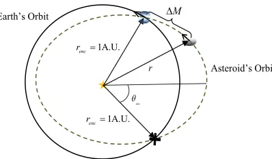
Fig. 3: Orbital geometry of the coplanar model.
As shown in Fig. 3, an Earth-crossing coplanar asteroid has two intersections (points of MOID equal 0) with the Earth’s orbit. These are found when the asteroid is at 1 AU from the Sun. Since the distance r from the Sun to the asteroid is known, the equation of the orbit in polar coordinates yields the true anomaly of the two encounters θenc:
1 1
cos enc
p e θ = ± −
−
(8)where p a= (1−e2) is the asteroid’s semi-latus rectum and the unit length in Eq.(8), and any of the following formulas in this paper, has been normalized to 1 AU.
With the true anomaly of the encounter θenc known, the velocity at the encounter can now be defined by using the
normal and radial components of Keplerian orbital motion:
( )
sin enc Sun r enc v e p µ θ= (9)
( )
(
1 cos)
enc Sun n enc v e p µ θ
= + (10)
where vrenc and enc n
v are the radial and normal velocity at the MOID point. Using Eq. (8) and Eqs.(9)-(10), the encounter velocity can be rewritten in a more suitable form:
(
)
(
2 1 2)
enc Sun r
v e p
p µ
= − − (11)
enc
n Sun
v = µ p
(12)
Whenever the Earth-coplanar asteroid meets the Earth at θenc, the velocity of the asteroid relative to the Earth will
then be
(
enc,
enc)
r n enc
v v −ω⊕⋅r with the Earth moving at an angular velocity
Sun
ω⊕ = µ . This Earth encounter conditions will result on a hyperbolic motion of the asteroid relative to the Earth with an excess velocity as:
(
3
1
2
)
Sun
v∞ =
µ
−
a
−
p
(13)Asteroid’s Orbit
1A.U.
enc
r =
Earth’s Orbit ∆M
3.1.2. Final Earth Insertion
If MOID is zero or almost zero, the Earth encounter could be easily tuned by a phasing manoeuvre so that the altitude during the Earth fly-by is some given minimum distance (chosen here to be 200km) above the Earth’s surface. At this minimum altitude a final insertion manoeuvre could be performed.
The notion of targeting asteroids towards the Earth may raise some concerns with regards to a possible
enhancement of the impact threat. Clearly, changing the orbit of a large NEO could potentially be a threat to Earth, although engineering the orbit of large objects may also be unfeasible. Thus for this objects transferring mined resources may provide the best and only option. On the other hand, for smaller bodies the impact hazard can be mitigated since bodies of tens of meters of diameter should completely ablate in the atmosphere[20]. Thus, bodies in the order of 10 meters diameter may be perfect targets for first capture demonstrator missions.
A parabolic orbit is assumed here to be the threshold between an Earth-bound orbit and an Earth escape orbit. Hence, the ∆v necessary for an Earth capture ∆vcap at the perigee passage results in:
2
2 2
cap
p p
v v
r r
µ⊕ µ⊕
∞
∆ = + − (14)
where
v
∞ is the hyperbolic excess velocity described in Eq.(13) and rp is the pericentre altitude (i.e.,r⊕+200km).Finally, the sum of Eqs.(7) and (14) provides the total ∆v budget for a two-impulse transfer to Earth. 3.1.3. Keplerian Feasible Regions
As noted earlier, the integration in Eq.(6) yields the probability of an asteroid to be found within a specified Keplerian region. By rearranging Eqs.(7) and (14), we can now define the regions from which transfers to Earth cost less than a given limit ∆vthr. Fig. 4, for example, shows the Keplerian region in the plane {a,e} where asteroid
Fig. 4: Keplerian {a,e} space reached by a maneuvre of 2.37 km/s (i.e., Moon’s escape velocity). Superimposed are all near Earth asteroids known within the {a,e} space as of April 2010.
Fig. 4 shows three different lines (solid, thick-dotted and thin-dotted line) delimiting an area in the {a,e} plane. The solid line results from expressing Eq.(14) as an explicit function of the semi-major axis a and ∆vcap necessary for
an Earth capture:
(
,)
1 1 3 1 2 24
cap
s
v e v a
a a µ
∞
∆ = − − −
(15)
where the hyperbolic excess velocity v∞ is defined as:
2
2 2
p p
cap
v
r r
v
µ⊕ µ⊕∞
=
∆ + −
(16)Equation (15) therefore yields the value of eccentricity for which an asteroid with semi-major axis a can be captured with a manoeuvre ∆vcap at the perigee passage. Asteroids with semi-major axis a, but eccentricity lower
than the result provided by Eq.(15) should be captured with a manoeuvre lower than ∆vcap. Thus, if ∆vcapis set to
the maximum allowed manoeuvre ∆vthr, the eccentricity resulting from Eq.(15) is also the maximum allowed
eccentricity, emax= ∆e v a
(
thr,)
, i.e., solid line in Fig. 4 when ∆vthr=2.37 km/s.Eccentricities lower than emax require lower ∆v manoeuvres to be captured at the Earth, but there is a geometrical
limit to the minimum Earth insertion manoeuvre∆vcap.The minimum ∆vcap occurs when the encounter geometry is
such that the intersection is at the line of apsis. With this geometry only one intersection point exists, and lower eccentricities imply orbits with no Earth-crossing points (see Fig. 4). The minimum allowed eccentricity for an orbit with semi-major axis a is therefore:
-1 -0.5 x 0 0.5 1
3 5 3 2 5 2 1 5 1 0 5 0 0 5 1
(
)
max , threshold
e a v∆
( )
mine a
-1 -0.8 -0.6 -0.4 -0.2 0 0.2 0.4 0.6 0.8 1 -1
0.8 0.6 0.4 0.2
0
0.2 0.4 0.6 0.8
( ) (
(
)
)
min
1 1 if 1 1 1 if 1
a a
e a
a a
− ≥
= − <
(17)
so that, if a≥1,the periapis radius is 1 (see thin-dotted line in Fig. 4), and, if instead a<1,the apoapsis is 1 (see thick-dotted line in Fig. 4).
Once the analytical expressions for the maximum and minimum eccentricity emax and emin are known, the
maximum and minimum allowed semi-major axis a can be computed by finding when emax
(
∆
v
threshold,
a
)
=emin( )
a
occurs. The latter equation results in a second degree polynomial with the following two solutions:(
)
min 2 max 1 1 2 threshold s s a v v v µ µ ∞ ∞ ∆ = − ± (18)where v∞ is defined as in Eq.(16) and amin correspond to the positive sign while amax corresponds to the negative.
Inside this delimited area within the {a,e} Keplerian space, we can ensure that the coplanar capture manoeuvres will be lower than the limit threshold ∆vthr. Thus, the reminder impulse,
∆vinc(a,e,∆vthr)=∆vthr-∆vcap(a,e) , (19)
can be used for changing the orbital plane of any available objects.
From Eq.(7) one can see that the cost of changing the orbital plane of a given asteroid is not only defined by the initial {a,e,i} of the asteroid, but also by the argument of the periapsis ω. The reason for this is that the velocity at the crossing plane vplX is the velocity at the line of nodes of the asteroid, whose orientation within the orbit of the
asteroid is defined by ω. Now, for a given orientation, or specified ω, the optimal location for a change of plane is the furthest node from the Sun, since this corresponds to the lowest velocity, and therefore, minimises Eq.(7). This then concludes that the optimal orientation of an asteroid for changing its plane to an inclination of 0 degrees is such that the line of nodes is the line of apsis, while the worst orientation is such that the line of nodes is the semilatus rectum.
Considering the worst orientation, the maximum inclination from which asteroids can be placed into a coplanar orbit is:
(
)
(
)
(
)
1 max_ 1/2 2 , ,, , 2 sin
2 1
inc thr
p thr
S
v a e v
i a e v
e p µ − ∆ ∆ ∆ = ⋅ + (20)
Thus, any orbit with an inclination lower than imax_p, no matter the orientation (i.e., ω), has a two-impulse transfer
to Earth with a ∆v budget lower than or equal to ∆vthr. The small crosses shown in Fig. 4 represent the surveyed
asteroids with inclinations lower than the resultant from Eq.(20).
(
)
(
)
(
)
(
)
1 max_ 1/2 , , , , 2 sin1 2 1 a inc thr r thr S
v a e v
i a e v
e a e µ − ∆ ∆ ∆ = ⋅ − + (21)
Thus, any asteroid with an inclination higher than imax_ra, no matter the orientation, cannot be transported to Earth
with a ∆v budget lower than or equal to ∆vthr.
For inclinations between imax_p and imax_ra only a fraction, between 0 and 1, of asteroids will statistically have the
orientation required for a change of inclination within the ∆v budget. In order to compute this fraction, one can start by calculating the range of true anomalies that allow a change of plane within the required ∆v. A true anomaly allowing the change of plane refers to a true anomaly for which if the ascending/descending node lies in that angular position, then the inclination maneuvre is possible with the allowed ∆v budget. Note that if the descending node lies at νdthe ascending node will lie at νd+π, and that the point chosen for the maneuvre would always be the position
with the lowest orbital velocity.
Since the NEO’s argument of the periapsis ω has been assumed to be uniformly distributed, the fraction of feasible true anomalies is equivalent to the fraction of feasible orientations. The following equation can then be written:
(
)
(
)
( )
2
1 , , 1
2 cos
2 2 sin 2 2 2
, , ,
inc thr
S
inc thr
v a e v
p e
i
e e
f a e i v
π µ π − ∆ ∆ − − − ⋅
∆ = (22)
which describes the probability to find an asteroid with the required orientation for a change of plane within the ∆v limit for inclinations between imax_p and imax_ra.
3.1.4. Probability to find an Accessible Asteroid
In previous sections we have defined the sequence of impulses in the transfer and the regions delimiting the set of starting orbits {a,e,i} from which the Earth is accessible under a total ∆v lower than a limit threshold. We can now compute the probability to find an object with these initial conditions by integrating the following equation:
(
)
max max max_(
)
max max max_(
)
(
)
min min min min min_
2 0 , , , , , , ,
P ra
p
a e i a e i
imp thr a e a e i inc thr
P ∆v =
∫ ∫ ∫
ρ a e i di de da⋅ ⋅ ⋅ +∫ ∫ ∫
ρ a e i f⋅ a e i v∆ ⋅ ⋅di de da⋅ (23)Equation (23) estimates the probability to find accessible resources under a given ∆vthr by using a two-impulse
transfer and a NEO orbital distribution as defined in section 2.2. Note that the dependence of P2imp with ∆vthr is not
only in the fraction finc but also in the limit of integrations, which have functional dependencies as follow:
(
)
(
)
(
)
(
)
(
)
min max min max max , ,0 , ,
thr thr
thr thr
thr
a v a a v
e a v e e a v i i a e v
∆ ≤ ≤ ∆
∆ ≤ ≤ ∆
3.2
As shown in One-impulse Transfer Fig. 4, if the asteroid is coplanar with the Earth orbit, two orbital crossing points will always exist, as long as the periapsis and apoapsis of the asteroid’s orbit are smaller and larger than 1 AU, respectively. On the other hand, if the asteroid is not coplanar with the Earth’s orbit, only specific values of the angle of the periapsis ω will render an orbital intersection or a MOID small enough for a capture to be possible (see Fig. 5).
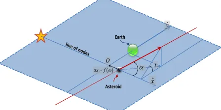
Fig. 5: Representation of all possible orientations of an orbit as a function of argument of the periapsis ω. The figure shows two orbital planes, one for the Earth’s orbit and one for the asteroid’s orbit. By continuously changing the argument of the periapsis, all possible orientations of the asteroid orbit in the plane are yielded. The two crosses
mark the Earth orbital crossing points which are possible only for four different values of the argument of the periapsis ω. Two arrows show the argument of the periapsis ω for one of the four configurations.
As shown by Fig. 5, only 4 specific values of ω yield a MOID equal to zero (i.e., an intersection between the two orbits). Except if the semilatus rectum p is equal to 1, in which case there will be only two values of ω yielding two simultaneous crossing points. Equation (8) already provided the two possible true anomalies that give the asteroid a distance of 1AU from the Sun. Therefore, for the orbital intersection to occur in the non-ecliptic asteroid case, one of these two angles is required to coincide with the line of nodes, i.e., the straight line where the two orbital planes meet. This yields four different arguments of the periapsis ω for which the MOID is 0:
{
}
0
MOID enc enc enc enc
ω = π θ− θ −π θ −θ (24)
Close to the values of ωMOID0, the variation of MOID as a function of periapsis argument can be approximated
linearly [19, 21]. With the axis shown in Fig. 6, the motion of the Earth and the asteroid can be well described using a linear approximation of the Keplerian velocities of the two objects at the line of nodes. This defines two straight line trajectories, and thus, the minimum distance between these two linear trajectories can be found.
ω
i
Earth’s Orbital Plane
Asteroid’s Orbital Plane
i α
ˆ
x
ˆ
y
( )
x f ω ∆ =
O
Earth
[image:14.612.197.433.155.314.2] [image:14.612.202.426.586.698.2]The minimum distance can then be written as an explicit function of ∆x (i.e., distance between the centre of the coordinates described in Fig. 6 and the point at which the asteroid crosses the Earth orbital plane), which can also be described as a linear function of the argument of the periapsis ω. Finally, an expression such as:
( )
( )
0 2 2 min 1 tan sin MOID MOID i ω ω α − = + (25)yields an approximate value of the MOID distance. The expression min[|.|] denotes the minimum value of the absolute differences with any of the angles ωMOID0 and the tangent of the flight path angle can be calculated as:
( )
(
)
22 tan 1 p e p
α
=− − (26)
For a complete derivation of a similar formulae, the reader can refer to Opik’s work [19] or alternatively to Bonanno’s work [21]. Note that Eq.(25) is valid only for values of ω close to any of the values of ωMOID0 from
equation (24). Fig. 7 shows, as an example, the evolution of the MOID distance as a function of periapsis argument for the elliptic orbit plotted in Fig. 5 (i.e., a=1.1AU, e=0.8,i=30o). The figure compares the results of the MOID
calculated by means of Eq.(25) with the results of a numerical algorithm that finds the MOID by minimising the distance between two positions defined by the true anomaly of each orbit. As can be seen, Eq.(25) yields a very good approximation of the real MOID when the MOID is small. Clearly, the error from this formulation increases for very low inclinations and very low eccentricities, but it is still tolerable for inclinations of 0.1 degree and eccentricities of 0.01.
Fig. 7: Comparison between the analytical and numerical approaches to compute MOID. 3.2.1. Capture at MOID Point
Now that it has been shown that the analytical approximation of MOID is a reliable way of assessing the distance between two orbits, we can define the maximum MOID at which the capture of an object is possible given a limiting ∆v budget. Equation (14), in section 3.1.2., defined the required Earth capture manoeuvre ∆vcap as a function of the hyperbolic excess velocity v∞ andthe pericentre altitude rp. The latter can also be expressed as an explicit function of
the hyperbolic velocity v∞ and the impulsive manoeuvre:
0 50 100 150 200 250 300 350
10-3 10-2
10-1 100
Argument of the Periapsis, deg
M
O
ID,
AU
0 50 100 150 200 250 300 35010-2 10-1 100 101 102 D if fe ren ce ,%
Difference between numerically and analitically calculated MOID
(
)
22
2 2
8 cap p
cap v r
v v
µ
⊕∞
∆ =
− ∆ (27)
Since equation (27) refers to non-coplanar asteroids, the hyperbolic velocity v∞ needs to be calculated as:
( )
(
3 1 2cos
)
S
v∞ = µ − a− p
⋅
i
(28)This expression can be derived by noticing that the relative velocity at the encounter for a non-coplanar asteroid can be expressed as:
(
vrenc,vnenc⋅cos( )
i −ω
⊕⋅r venc, nenc⋅sin( )
i)
.Finally, in order to know the maximum MOID at which a direct capture is possible, the distance rp needs to be
corrected by the hyperbolic factor, i.e., factor that accounts for the gravitational attraction of the Earth during the asteroid’s final approach to the Earth. This results on:
2 MOIDcap p 1
p r
r v
µ
⊕∞
= + (29)
Note that if the perigee altitude resulting from Eq.(27) is smaller than the radius of the Earth, this would mean that the capture of that particular body is not feasible under that particular ∆v threshold used. In fact, the feasible limit for a fly-by was set to 200km altitude from the surface of the Earth, also to account for the Earth’s atmosphere.
3.2.2. Fraction of Capturable Asteroids
The previous section provided the means of calculating the MOID at which capture is possible as a function of
cap v
∆ . Using the linearly approximated MOID in Eq.(25), we can see that within a distance ∆ωof ωMOID0 such as:
( )
( )
2 2 1
MOID tan
sin
cap i
ω
α
∆ = ⋅ +
(30)
a direct capture of the asteroid is possible, since the minimum orbital distance is ensured to be smaller than MOIDcap,
and thus, the capture impulse should be smaller than ∆vcap. One may think then that the total range at the neighbourhood of ωMOID0 is 2∆ω, and since there are 4 different ωMOID0, the total range of ω at which capture is
possible should be 8∆ω. This is generally correct, but attention must be payed when overlapping of the ranges occurs. If the semilatus rectum p is close to 1, the values θencand π-θenc are also close and their ranges (θenc±∆ω and
π-θenc±∆ω) may overlap. A correction is applied in those cases.
The fraction of asteroids with given {a,e,i} that can be captured with a given ∆vbudget is then:
(
, ,)
8(
, ,)
2
lowMOID
a e i
f a e i = ∆ω π
⋅ (31)
without the overlap correction. The fraction flowMOID provides the fraction of material with Keplerian elements {a,e,i}
that could be captured with a single manoeuvre (≤∆vcap) at the Earth. Capture of asteroid material by means of only
3.2.3. Keplerian Feasible Regions
The capturable feasible regions using one-impulse transfers in the {a,e} subspace are the same as in section 3.1.3. The only difference between the feasible volume {a,e,i} of the two-impulse and the one-impulse model lies in the inclination. Since no change of inclination is required, the maximum inclination from which asteroids can be captured is greatly increased. The limit threshold can be computed by realising that v∞ calculated as in Eq.(28) must
be equal to v∞ calculated as in Eq.(16), thus:
(
)
1 2max , , cos 1 3 1
2 S
v
i a e v a
p
µ
− ∞
∆ = − −
(32)
where v∞ is calculated as in Eq.(16) with an rp =r⊕+200km.
3.2.4. Probability to find an accessible asteroid
Finally, the probability to find an asteroid in an accessible initial orbit (i.e., accessible by using one-impulse transfer) is:
(
)
max max max(
)
(
)
min min
1 0 , , , ,
a e i
imp thr a e lowMOID
P ∆v =
∫ ∫ ∫
ρ a e i f⋅ a e i di de da⋅ ⋅ ⋅ (33)where P1imp functional dependency with ∆vthr is in the limits of the integration, which are defined by Eqs.(18), (15),
(17) and (32). 3.3
At this point, the probability to find accessible objects (Eqs.(23) and (33)) and the size population model in section 2.1. can be combined in order to estimate the available material that could be exploited for future space ventures. The accessible material will be mapped as a function of the limiting ∆v budget, and as described in the previous two sections, once a ∆v threshold has been defined, the probability to find accessible material is computed by integrating Eq.(23) and Eq.(33) for two and one impulse transfers respectively. When the probabilities P2imp and
P1imp are known, the average accessible mass of near Earth object material can be calculated by multiplying these
probabilities with the total mass of asteroids yielded by Eq.(5) considering objects between 32 km (i.e., largest Near Earth object known today) and 1 meter diameter.
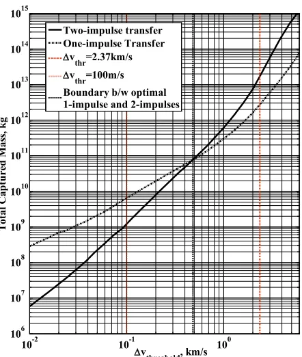
Average Accessible Mass.
Fig. 8: Average accessible asteroid mass for exploitation of resources as a function of ∆v threshold. The results in Fig. 8 allow a direct comparison between lunar and asteroid resource exploitation. For a∆vthreshold equal to the Moon’s escape velocity (i.e., 2.37 km/s) the average total accessible asteroid material is of the order of 1.75x10¹³ kg using a two-impulse transfer as described in this paper. Approximately, 3x10¹²kg of material could also
be captured during Earth fly-by, without having to modify the orbit geometry of these objects. Note that the so-called accessible material is made up in reality of many small asteroids and statistical fractions of larger objects (i.e., for example, the 1/1000 chance to find a large object counts in Fig. 8 with a 1/1000 fraction of its mass). Hence, the values represented in Fig. 8 do not provide yet any conclusive statement on the feasibility of the concept, but allow us to see a clear limit on the material that could actually be accessed from Earth for its utilization. For example, all the exploitable asteroid material within an energy lower than the cost of transfer from the Moon (i.e., ∆vthreshold≤2.37 km/s) is actually less than the mass of an object with 2.5 km diameter (assuming average density).
Even if this ∆vthresholdprovides potentially access to orders of magnitude more material at the Moon (i.e., mass of the Moon ~7.36x10²²kg), the main advantage of asteroid resources with respect lunar resources is that asteroid
material can be exploited at a whole spectrum of ∆v, rather than the minimum threshold required for lunar material (i.e., 2.37 km/s). For example, 6.4x10⁹kg of asteroid resources could still be exploited at a
threshold v
∆ of only 100 m/s by using a serendipitous capture such as the one described by the one-impulse transfer. Lunar material instead requires an energy threshold to overcome the Moon’s gravity well (i.e., a ∆v of 2.37 km/s). In addition, the Moon is believed to be a relatively resource-poor body [2], therefore asteroid resource exploitation above 2.37 km/s may still be an attractive option if valuable materials are available not found on the Moon.
10-2 10-1 100
106 107 108 109 1010 1011 1012 1013 1014 1015
∆v
threshold, km/s
Tot
al
C
ap
tu
re
d M
as
s, k
g
Two-impulse transfer One-impulse Transfer
∆vthr=2.37km/s
3.4
Previous sections have assumed that if the orbital intersection exists, then the asteroid would eventually meet the Earth. This statement may be true if the time available to transfer the asteroid is not constrained, but for realistic scenarios this does not occur. Therefore, some analysis on the cost of the manoeuvring necessary to ensure the encounter opportunity must be performed.
Phasing Maneuvre
For a more realistic transfer scenario, in which the orbital phasing is also considered, an additional impulsive manoeuvre may be necessary in order to provide the correct phasing to the asteroid. This manoeuvre is generally small and must be provided as early as possible, so that the secular effect due to the change in period yields the orbital drift necessary for the asteroid to be at the Earth orbital crossing point at the required time. Hence, if only secular effects are considered [22, 23], which is regarded as a good approximation for the level of accuracy intended in this paper, the phasing manoeuvre should correct the difference in mean anomaly ∆M that exists for the intended encounter (see Fig. 3). This is expressed as:
(
e m)
M n t t
∆ = ∆ ⋅ − (34)
where ∆n is the change of mean motion of the asteroid due to the phasing manoeuvre and (te-tm) is the time-span
between the manoeuvre (tm) and the encounter (i.e. time at which the Earth is at the crossing point te). The change in
mean motion of the asteroid can be defined as:
(
)
3 3Sun Sun n a a a µ µ δ ∆ = − + (35)
where δa is the change of semi-major axis of the asteroid due to the impulsive manoeuvre. Using the Gauss planetary equations[24], δa can be expressed as:
0 2 2 t S a v a v
δ
δ
µ
= (36)where δvt is the tangential component of the impulsive manoeuvreand v0 is the orbital velocity at the point at which
the impulsive manoeuvre is applied. Eq.(36) seems to indicate that the optimal position for a phasing manoeuvre is the periapsis, since this is the point at which the orbital velocity v0 is maximum. This is generally true, except for
cases in which the term (te-tm) of equation (34) drives the optimality of the phasing manoeuvre.
Finally, rearranging Eq.(34), (35) and (36), the phasing manoeuvre necessary to drift the asteroid through ∆M angular position at time te, given a impulsive manoeuvre at time tm, can be expressed as:
(
)
0 1 3 2 2 3 2 S S t S e m v aa v M
t t a
µ µ δ µ = − ∆ + − (37)
which provides a good estimation of the cost of the phasing manoeuvre to target an Earth encounter.
Considering an Earth-asteroid configuration such as in Fig. 3, an algorithm was implemented that computes the fraction of mean anomalies inside the asteroid orbital path that can be phased with the Earth with a δvt smaller than a
the crossing point from which ∆M is measured. Also a time constraint needs to be specified, which defines the maximum allowed manoeuvre time tmax
m. Then, the algorithm computes the δvt necessary to cancel not only the ∆M
gap at time te, but also all other possible encounters opportunities, which are defined by the times at which the Earth
is at the crossing points during the time-span available. For each possible encounter two manoeuvre times are considered; the first available periapsis passage and tmax
m. This procedure is repeated for many different angular
positions ∆M at te, from which then the fraction of the orbit that can be phased under a ∆v limit is calculated.
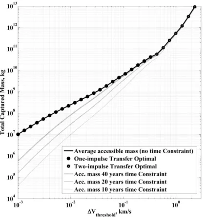
[image:20.612.202.413.176.399.2]Fig. 9: Time constrained and unconstrained accessible mass.
Fig. 9 includes the effect of 40, 20 and 10 years time constraints on the accessibility of asteroid resources. The figure also shows accessibility of asteroid material without considering any time constraint (also shown in Fig. 8), but this time only the results of the optimal transfer strategy are shown for each ∆v threshold. From the results in Fig. 9 it can be concluded that the free phasing assumption during the description of the transfer models is a good approximation for relatively large ∆v thresholds. At low ∆v thresholds some early manoeuvring may be required. Note that a 40-year trajectory may not necessarily be envisaged as a trajectory requiring 40 years to be completed. This only suggest the necessity to provide early shepherding manoeuvres, allowing asteroids to have the right phasing conditions with Earth. Years later, a short sequence of manoeuvres can be provided to achieve a final capture of the asteroid or its mined material.
4.
One of the important issues not resolved by the results shown in ACCESSIBILITY OF ASTEROIDS Fig. 8 and Fig. 9 is the number of missions that would require exploiting all or part of the accessible asteroid resources. This issue is of key importance, since if a given resource is spread in a large number of very small objects, gathering all of them may become a cumbersome task, and therefore not economically worthwhile.
the binomial distribution. In this particular case, for which P is a very low probability and n a very large number of asteroids, Poisson distribution (a limiting case of the binomial distribution when n tends to infinity) represents a very good approximation of the statistical behaviour of the problem. Therefore, the probability g(k,λ) to find k asteroids when the expected number is λ can be described by:
( )
, !ke g k
k
λ
λ
λ
= − (38)The expected number λ, or average number of accessible asteroids, can be calculated as:
(
Dmin)
N D(
min D Dmax)
Pλ = ∆ < ≤ ⋅ (39)
where ∆N is the total number of asteroids with diameters larger than Dmin and smaller than Dmax (Eq.(2)) and P the
probability to find objects within a given Keplerian region. In the following, ∆N will keep Dmax fixed to the 32-km
diameter, while Dmin may vary to modify the value of λ as required.
An integration such as:
( )
,NEA
n
g k
λ
dk∞
⋅
∫
yields the probability to find at least nNEA asteroids when the expected value, or average, was λ. By finding then the
value of λ that yields an accumulative probability of 50%,
(
)
(
, min)
50% NEAn
g k
λ
D dk∞
⋅ =
∫
, (40)we can estimate the median diameter of the smallest object in the nNEA set. This procedure can also be repeated with
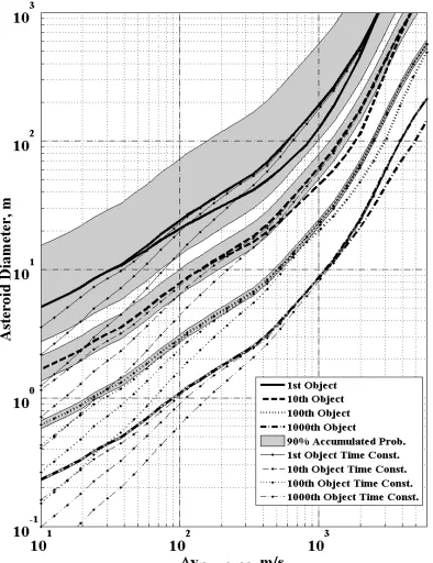
[image:21.612.215.412.446.702.2]accumulative probabilities of 95% and 5% to obtain the 90% confidence region. The results of this procedure can be seen in the following figure.
Fig. 10 shows the median diameter of the first, tenth, hundredth and thousandth largest accessible asteroid in the near Earth space, together with the 90% confidence region of each one of these objects. Note that the 90%
confidence regions account only for the statistical uncertainty of finding k asteroids within a population of n objects, assuming that the population is perfectly described by Eq.(1). The figure also shows the median diameter considering a 2/3 drop in the number of small asteroids as estimated by Harris [25], this is represented by the lower branch in each asteroid set of data. This second population size distribution of asteroids was represented by a three slope power law distribution matching with Eq.(1) at 1-km and 10-m, while providing a 2/3 drop on the accumulative number of asteroids at 100-m. Finally, Fig. 10 also shows the results by considering 40, 20 and 10 years of time constraint in the transfer time, represented as the three departing lines from the main set of data.
The information in the figure can be read as follows: let us set, for example, the ∆v threshold at 100 m/s, the largest accessible object has a 50% probability to be equal to or larger than 24 meters diameter, while we can say with 90% confidence that its size should be between 72 meters and 12 meters. We can also see that when accounting for a population of asteroids as estimated by Harris [25] the median becomes 20 meters instead of 24 meters. Finally, we also see that when time constraints are included and phasing maneuvre are estimated as described in section 3.4., the median diameter decays to 23 meters when the constraint is set to 40 years, 20 meters if the constraint is 20 years and 13 meters if the limit is at 10 years (solid-dotted lines). The following set of data in the decreasing ordinate axis is the group referring to the 10th largest object found within the region of feasible capture given by a ∆v threshold of
100 m/s, whose median diameter is at 8 meters diameter. The 100th largest object is foreseen to have a diameter of 3
meters and 1000th largest of 1 meter.
5.
Figures 8 to 10 provide a good basis to understand the accessibility of general asteroid material, with no distinction yet on the type of material expected to be found. The results shown, especially in
FINAL DISCUSSION
Fig. 10, seem to imply that there is ample material that could potentially be exploited at a relatively low energy, at least if compared with the energetic cost of exploiting resources at the Moon. Perhaps the most important characteristic of the concept is its scalability. As noted earlier, mining the Moon would require a minimum investment of energy to transport the material from the bottom of the Moon’s gravity well. Many asteroids are also expected to be accessible with equivalent investment of energy or lower. More importantly, the level of energy or ∆v necessary to exploit modest asteroid resources can be as small as necessary for available technology to manage.
Earth-benefit from a judicious use of multi-body dynamics (e.g., interplanetary highways [27]). These results do not necessarily mean that the patched conic is not a correct approximation, but instead, that it needs to be put in context for very small ∆v.
For larger ∆v, instead, the benefits of judicious use of gravitational perturbations are less important. However, large ∆v transportation costs are here overestimated due to the very poorly designed change of plane manoeuvre. As discussed previously, the change of plane, as modelled here, ensures that a non-coplanar asteroid will intersect the orbit of the Earth (if rp<1 and ra>1), while allowing the use of analytical formulae to compute ∆v cost. This was
necessary in order to analytically define the feasible Keplerian space from where ∆v transfers could be achieved at a ∆v lower than a given threshold. Ideally, a more optimal asteroid transfer would reduce the Earth MOID to zero, ensuring an intersection with the Earth’s orbit, without the over-penalising costs of changing the inclination of the initial trajectory. This, at a minimum, requires a numerical optimization of a Lambert arc transfer. A more realistic transport trajectory would however be designed by optimizing a low-thrust trajectory, by means, for example, of optimal control theory [28]. This would be especially desirable if considering that the low-thrust propulsion systems provide the highest efficiency at delivering change of linear momentum, and thus it would be the logical propulsion choice for a robotic mission to transport asteroid resources. The ∆v penalty posed by the analytical approximation used at the two-impulse transfer model can be assessed by comparing the analytical model with optimized free-phase Lambert arc transfers. Optimizing Lambert arcs is a computationally costly procedure and it would have been unsuitable in this paper, where it was required to perform millions of transfer evaluations. Nevertheless, a set of 3000 randomly distributed {a,e} conditions with a predefined ∆v cost at 1.18, 2.37 and 4.74 km/s were analysed and weighted by the NEO density function. This analysis reveals that ∆v axis in Figures 8 to 10 may be under-scaled by a factor, at worst, of 1.5 (e.g., the mass or asteroid size at 2 km/s ∆v could possibly approach the result at 3 km/s in a fully optimized scenario).
5.1
Asteroids have a very diverse composition and, thus, the possible uses of the different accessible objects (i.e., as shown in
Available Resources
Fig. 10) will always depend on the particular object characteristics. Any available space resource however can be envisaged to be put to good use, since for example, lacking any better option, bulk material (regolith and unprocessed material) could be used as radiation shielding, which would reduce the hardening requirements to survive in space and as a consequence reduce the mass launched into space. Nevertheless, one can envisage much more disruptive uses for some particular resources, such as water and volatiles, which could be used to sustain human life in space, as well as a rocket propellant, semiconductors that could be used to build in-situ solar cells and metals used for space structures.
Providing estimates on the amount of resources for different valuable materials can only be based on statistical estimates from spectroscopic surveys and meteoroid recoveries. While spectroscopic surveys of Near Earth Asteroids show a very wide diversity of spectral classes [30], only meteoroid recoveries provide an accurate account of the materials available in space [31]. The latter however have a clear body strength bias (i.e., weaker objects ablate in the atmosphere) and are quickly weathered if not recover soon after atmospheric entry.
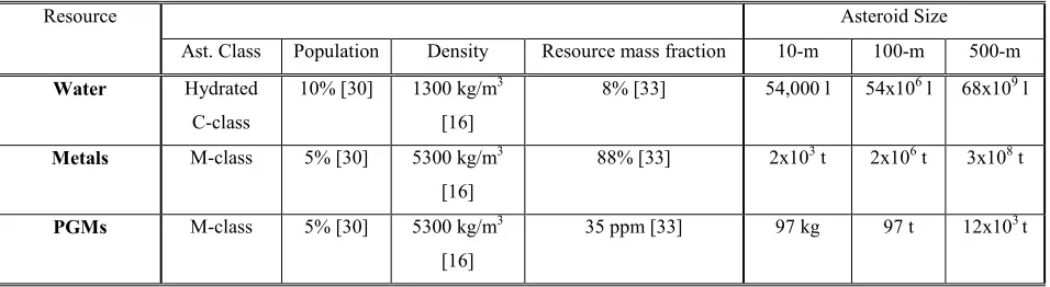
[image:24.612.66.544.499.630.2]It is not the purpose of this paper to provide an accurate census of object types and resources availability, primarily because with the current knowledge of asteroid composition and their availability on different orbits is inaccurate. On the other hand, a few examples of possible resource availability at different ∆v thresholds may cast some more light on the usefulness and possibilities of the exploitation of asteroid resources. The following table is provided only as an example of the amount of material that could be found in different sized objects. Table 1 assumes that water should be extracted from hydrated carbonaceous asteroids, while metals and platinum group metals (PGM) would be extracted from M-class objects. This however does not imply that these resources are only available in these types of objects. Quite on the contrary, other asteroid classes, such as for example S-class [32], may contain more interesting combination of volatiles, metals and semiconductors [31], albeit volatiles and metals would likely be found at lower abundances than for the examples described on Table 1.
Table 1. Example of possible resources on different asteroid classes.
Resource Asteroid Size
Ast. Class Population Density Resource mass fraction 10-m 100-m 500-m
Water Hydrated
C-class
10% [30] 1300 kg/m3
[16]
8% [33] 54,000 l 54x106 l 68x109 l
Metals M-class 5% [30] 5300 kg/m3
[16]
88% [33] 2x10³ t 2x10⁶ t 3x10⁸ t
PGMs M-class 5% [30] 5300 kg/m3
[16]
35 ppm [33] 97 kg 97 t 12x103 t
if the object turns to be an hydrated carbonaceous asteroids a million litres of water could possibly be extracted (considering, as in Table 1, an asteroid of density 1300 kg/m3 [16] and 8% [33] of its weight in water). However, if
this object is a M-class asteroid (density 5300 kg/m3 [16]), of order thirty thousand tonnes of metal could potentially
be extracted and even a tonne of Platinum Group Metals (PGM) (88% of metal assumed and 35ppm of PGM [33]). The latter resource could easily reach a value of fifty million dollars in Earth’s commodity markets [34].
Note from the examples in Table 1 that hydrated C-class and M-class only cover 15% of the asteroid population, implying that this hypothesized 24-m object has only a 15% probability of being one of these two classes. As previously noted, this does not mean that there is an 85% chance that the asteroid would be of no use, or that the 85% remaining population has less resource interest. S-class asteroids, accounting approximately for 40% of the NEA objects, could very well become the most interesting targets to exploit since they likely contain relatively good abundances of semiconductors, metals and even volatiles such as oxygen, including perhaps water. S-class may also contain PGM, albeit at a lower abundance than in M-class. One could possibly imagine the utilization of a 24-m S-class object to provide between 1 to 4 thousand tonnes of iron to be used as a structural support for the 1.5 km2
silicon solar array surface (build from the same object), which would generate a minimum of 1GWatt of power [35, 36]. The capability to exploit small S-class objects may perhaps allow solar power satellites to become commercially viable. Water could also be possibly extracted from S-class objects. Assuming a 0.15% of water [35], this would account for 30 thousand litres of water, which if we assume that a human being requires about 3 litres of water a day, from which at least 90% is recovered through recycling, there should still be enough water to sustain a crew of 25 people for 10 years, and perhaps no resupply of water would be required for the crew responsible to build the solar power orbital plant.
![Fig. 1: Accumulative size distribution of Near Earth Objects (from Stokes et al. [8])](https://thumb-us.123doks.com/thumbv2/123dok_us/1678466.121280/5.612.199.419.71.247/fig-accumulative-size-distribution-near-earth-objects-stokes.webp)
![Fig. 2: Theoretical Bottke et al. [9] NEO distribution. The figure shows the integrated projections of the function ρ(a,e,i) and a set of grid points coloured and sized according to the values of the NEO density](https://thumb-us.123doks.com/thumbv2/123dok_us/1678466.121280/7.612.108.505.99.319/theoretical-distribution-integrated-projections-function-coloured-according-density.webp)