Condition monitoring benefit for offshore wind turbines

Condition Monitoring Benefit for Offshore Wind

Turbines

Sebastian Thöns

Division 7.2 Buildings and Structures BAM Federal Institute for Materials Research

Berlin, Germany sebastian.thoens@bam.de

David McMillan Institute for Energy & Environment

University of Strathclyde Glasgow, UK dmcmillan@eee.strath.ac.uk

Abstract— As more offshore wind parks are commissioned, the focus will inevitably shift from a planning, construction and warranty focus to an operation, maintenance and investment payback focus. In this latter case, both short-term risks associated with wind turbine component assemblies, and long-term risks related to structural integrity of the support structure, are highly important. This research focuses on the role of condition monitoring to lower costs associated with short-term reliability and long-term asset integrity. This enables comparative estimates of life cycle costs and reduction in uncertainty, both of which are of value to investors.

Keywords: Condition Monitoring, Offshore Wind, Operation, Risk, Life Cycle, Cost

I. INTRODUCTION

There is likely to be a large increase of installed capacity of offshore wind power in the coming decade. Assuming the EU build rate during 2010 (883 MW installed [1]) can be increased to 1GW per annum and sustained until 2020, and assuming an average capacity of 3.4 MW per turbine [2], this would result in ~3,500 wind turbine assets in the water. This is a conservative figure compared to some highly optimistic estimates, but is still a huge number of assets. Economic asset management of such a high number of units in such harsh environmental conditions, both in the short and long term, is non-trivial.

This paper highlights the asset management challenges associated with this increased deployment by use of case studies, and proposes probabilistic methods to measure and reduce risk to investors and operators of offshore wind plant. Offshore reliability and associated operation and maintenance cost estimation is an area of keen interest to wind farm operators. There is a high degree of uncertainty associated with these costs, coupled with some evidence showing O&M expenditures broadly in-creasing in early life [3]. To control this trend and to achieve risk reduction, models need to be developed in order to predict what is a neglected and important part of wind farm life cycle cost.

II. OPERATION MACHINERY MODEL

A. Short-term Operation Machinery

Since operational information from offshore sites are sparse, the approach taken here is to examine data from

onshore maintenance records and adjust the downtimes, lost energy and failure rates to a level appropriate for offshore installations (there are precedents for this kind of approach such as [4]).

Previous studies showed how Markov chains coupled with Monte Carlo simulation provide a suitably flexible approach for modelling wind farm reliability and O&M ([5], [6]). The methodology has been successfully adopted by several other authors ([7], [8]) to solve similar problems. In this paper, the approach is utilised to produce a cost-benefit analysis of condition based maintenance.

B. Failure Modelling

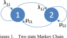
[image:1.612.387.498.420.484.2]

Following a reliability centred maintenance study (see e.g. [9]), failure rates for a set of wind turbines have been derived. Individual asset groups are then modelled by a Markov chain. For the simplest case, consider Figure 1, a two-state chain where state 1 is operational and state 2 is failed, failure rate of component is λ12 and repair rate is µ21.

Figure 1. Two state Markov Chain

The probability of remaining in each state during time step ∆t:

λ11∆t = 1 - λ12∆t (1)

µ22∆t = 1 - µ21∆t (2)

Probability of being in state 1 after time step ∆t:

P1(t+∆t) = P1(t) λ11∆t + P2(t) µ21∆t (3)

P1(t)’ = -λ12 P1(t) + µ21 P2(t) (4)

which degrade slowly over time, such components with bearings.

The asset categories used in this study differ from previous studies, which have focused on gearbox, electronics, generator and rotor [5]. These components have been revised on the basis of recent reliability centred maintenance (RCM) studies, and are summarised in Table I. The fault occurrence rate, θ, is derived on the basis of a utilities asset management system, which comprised 84 turbines and 255 operation years. The turbines are modern multi-MW machines within the range 3-5 years of operation. A fault occurrence is classed as anything that causes the wind turbine to stop functioning, no matter how trivial. Thus the database encompasses all failure events: from those requiring a very short maintenance visit, to those requiring cranage, additional specialist labour, and large component replacement cost. The top four components are modelled in this study, however tower is replaced with gearbox owing to the very low impact nature of most tower faults, which mostly relate to maintenance access systems.

C. Costs, Assumptions, Constraints

[image:2.612.321.555.71.147.2]

By analyzing maintenance databases, it is possible to extract many useful metrics which can be used for populating a maintenance cost model. The failure rate (λ) and mean time to repair (MTTR) are the most obvious metrics. In addition, it is possible to study the severity of faults and their likelihood. In this paper we consider minor and major failures, with associated probability (P(minor), P(major)) and cost (C(minor), C(major)). These are shown in Table II.

TABLE I. FAULT OCCURRENCE RATE BY ASSET GROUP – ONSHORE DATA

asset name θ (∆t=1 year)

Controller 2.362

Nacelle 1.391

Tower 1.221

Transmission 1.091

Gearbox 0.841

Hub 0.490

Parking brake 0.380

Hydraulics 0.360

Yaw 0.270

Generator 0.230

Pitch 0.220

Measurement (sensors etc) 0.210

Blade system 0.060

Switchgear 0.060

Over speed protection system 0.040

HV system 0.040

TABLE II. MODEL COST ASSUMPTIONS.MTTR IS BASED ON MAJOR FAULRES AND ASSUMES TIME BASED MAINTENANCE

Failure Mode λ(∆t=1 year) MTTR (days) P(minor) P(major) C(minor) € C(Major) €

controller 0.176 1 0.450 0.550 1995 16991

gearbox 0.180 7 0.978 0.022 16706 489768

nacelle 0.328 1 0.536 0.464 1093 2749

transmission 0.035 43 0.000 1.000 N/A 234098

Modelling of time based maintenance (TBM) is based on restoration of the Markov chain to fully operating condition once per annum. This incurs minor costs as shown in Table II. However in the event of an unplanned failure, a cost premium of 50% is applied to the incurred costs. This is broadly representative of specialized vessel hire and labour at short notice, and the possible need for fast fabrication and shipment of components, again in an unplanned, expedited manner.

The key assumptions underpinning the condition based maintenance (CBM) model are that via better maintenance planning, costs are kept to the values shown in Table II. In addition, the MTTR for a gearbox is reduced to 3 days and transmission to 7 days. Since the chief operational advantage of CBM is increased scope for planning, it is appropriate that modelling of CBM explicitly captures the effects of improved planning to reduce downtime and procure in a planned, low risk manner.

The energy yield model [5] is based on wind data simulated from a coastal location in the UK, as offshore data were not available [10]. The equivalent capacity factor is 35%. The main cost assumption is that the electricity production credit is €126/MWh. This is based on future reforms to the UK ROC system and is equivalent to 1.8 ROCs/ MWh.

[image:2.612.72.276.409.660.2]

The final constraint is offshore access. This is based on a probabilistic wave height model developed in [11] – see Figure 2. At the moment site access to offshore wind farms is generally constrained at wave heights of 1.5m or over. Thus all modelled maintenance actions (CBM, TBM and unscheduled) are affected by this constraint.

[image:2.612.324.543.503.661.2]

D. Case Study

In the case study we consider a 5MW offshore machine with failure rates and MTTF as shown in Table II. Multiple simulations are run at a time resolution of 1 day. Wind speed, energy yield, revenue generation, incurred O&M cost and weather constraint are all factored in as explained in previous sections. Since failure rates are expected to increase in the offshore environment, we increase λ and perform a sensitivity study to evaluate the two maintenance methods. The analysis is carried out for 2 cases:

• Case 1 (optimal CBM) – all 4 asset failure modes are subject to CBM (operating with reduced MTTRs and base costs described in section II c)

• Case 2 (realistic CBM) – gearbox and transmission are subject to CBM, but MTTRs are increased to 5 and 20 days respectively. For TBM, no cost premium is applied to nacelle and controller. Repair cost premiums for gearbox and transmission are inflated by only 10% instead of the 50% in case 1.

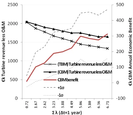
Figure 3 shows the impact on availability as λ is increased. It can be seen that despite the increase in λ, the CBM policy maintains availability at a much higher level. This shows the potential technical benefits of CBM. Interestingly, the results from the TBM policy are in the same ballpark as availability figures from round 1 offshore sites in the UK [11]. Figure 4 shows an economic benchmark between TBM and CBM. It is noted that for the starting values of λ (see Table 2), the CBM policy is approximately at economic parity with TBM. Only when failures begin to increase is the value of the CBM policy obvious. Figure 5 shows how Case 2 assumptions significantly alter the economics of CBM.

[image:3.612.333.553.52.242.2]

Figure 3. Case 1. Impact of increased failure rates on asset availability under time based and condition based maintenance.

[image:3.612.330.551.293.401.2]

Figure 4. Case 1. Economic benefit of condition based maintenance under model assumptions.

Figure 5. Case 1 vs. Case 2. Economic benefit of condition based maintenance under model assumptions.

III. STRUCTURAL INTEGRITY MANAGEMENT

The basic idea of the structural integrity management is the cost efficient mitigation of structural risks for securing the functioning of the support structure throughout the life cycle. Structural risks are characterized by low probabilities of failure but high consequences such as the loss of one plant or a wind park. The structural integrity management comprises in the operation phase the inspection and maintenance planning in combination the monitoring of the wind turbine structure.

[image:3.612.71.288.424.616.2]

On the basis of an optimization of a life cycle cost benefit analysis comprising the inspection, maintenance and repair costs, the failure costs and the costs of human safety usually the target reliabilities for the structures are determined (e.g. [14] and [15]). This optimization of the life cycle costs of a structure accounts for the boundaries in the context of the present code generation (see e.g. the Linds postulate, e.g. [16], [15]). The target reliabilities can then be compared to the results of the structural condition assessment and can serve as a basis for the determination of the inspection intervals (e. g. [17], [15], [18]).

The optimization of the life cycle costs must not be restricted only to the reliability level but can include further decision variables. Recently is has been shown that monitoring systems can significantly influence the expected life cycle cost of an offshore structure implying that monitoring systems give more certain information about the condition of the structure ([19]). Furthermore, the monitoring of the wind turbine and its structure is already a part of the regulation applying to an offshore wind park in the external economy zone in Germany ([12], [13]).

The aim of the following sections is to analyse the influence of monitoring systems first on the expected failure costs, i.e. on the risks, and second on the expected costs of the structural integrity management. For this aim the fundamentals of a life cycle cost benefit analysis are outlined in the section A and an expected monitoring benefit related to the failure costs and to the structural integrity management costs are derived. In section B the parameters, i.e. the decision variables, to be considered are derived and the optimisation aims are formulated. Section C contains then the outline of a case study and the results.

A. Long Term Structural Operation Model

The long term structural operation model consists of a life cycle cost benefit analysis including condition monitoring of a structure. A cost-benefit analysis includes the expected value of the life-cycle costs E C

[ ]

T , the

expected value of failure costs E C

[ ]

F , the expected costs of

the structural integrity management E C

[

SIM

]

comprising the

expected inspection costs E C

[ ]

I and repair costs E C

[ ]

R (Equation (1) and (2), building upon the approach of [17]). Such a life-cycle cost-benefit analysis involves various probabilistic and deterministic models. The risks are calculated on the basis of a structural reliability assessment in combination with the consequence scenario model. The expected inspection costs are determined applying a risk based inspection planning methodology and a cost model for the inspections. The probabilities of failure, inspection and maintenance actions are interconnected and are modelled with a decision tree.

[ ]

T

[ ]

F

[

SIM

]

E C =E C +E C (1)

[

SIM

]

[ ]

I

[ ]

R

E C =E C +E C (2)

It has been demonstrated in [19] that the reliability calculated with monitoring data and its associated models can be higher in comparison with the design data and models. This increase in reliability is caused by lower (model) uncertainties for the utilisation of the monitoring data for the case of low measurement uncertainties. By the change, i.e. the increase, of the structural reliability the expected life cycle costs are affected and Equation (1) is rewritten (Equation (3)). The expected costs of failure

M F

E C_ _ then additionally include costs associated to the loss of monitoring system.

M M M

T F SIM

E C_ _=E C_ _+E C_ _ (3)

The expected costs for the structural integrity management including monitoring E C SIMM  comprise, beside the expected inspection and repair costs, the expected and channel k dependent costs of the monitoring system

( )

M Sys

E C_ k _ and its installation E C InstM

( )

k  as well as the

monitoring system operation M Op

E C_ _. The operation costs

are discounted with the discount rate ir to the present value dependent on the time of cash flow t and are multiplied by the yearly probability of no failure (1−pF) (Equation (5)).

( )

( )

M M M

SIM I R

M M M

Sys Inst Op

E C E C E C

E C k E C k E C

 =  +  +

     

     

+ _{ }+ _{ }+ _{ } (4)

(

)

1

(1 )

1

M M

Op F Op t

r

E C p C

i

  = − ⋅ ⋅

  ₋ (5)

The expected failure costs and the expected costs for the structural integrity management can be calculated with this approach for both cases, namely a structure without a monitoring system and a structure with a monitoring system. Furthermore, an expected monitoring benefit E B

[ ]

M as the difference of the expected cost with and without monitoring (E C_ _ and E C_ M_) can be calculated (Equation (6))

[ ]

M

M T T

E B =E C_ _−E C_ _ (6)

B. Decision Variables and Optimization Aims

Various parameters influence the expected life cycle costs. The focus is here on analyzing the design parameters of a monitoring system.

Basically, the application of a monitoring system involves the decision where to monitor and how many components to monitor. This generic decision can formally written with Equations (7) and where D denotes the decision set consisting of n different component sets cSi.

{

S1, S2, , Sn

}

,

D= c c K c (7)

structural reliability analysis. This criterion constitutes the reduction of the probability of failure by the monitoring data

M f p

∆ which was analysed and determined in [19].

Two different optimization aims can be formulated with Equation (6). The first optimization aim is to maximize the benefit related to the expected failure costs, i.e. to the risks (Equation (8)) accounting for the decision variables. What is written here in the form of an equation constitutes the common association to the purpose of monitoring, namely that monitoring reduces the risks. Then the expected monitoring benefit related to the failure costs should be always positive.

(

)

(

)

(

)

(

)

, ,

arg max , ,

F

M

M C S f

M M M

F S f F S f

E B c p

E C c p E C c p

 ∆ =

 

   

= _ ∆ _− _ ∆ _ (8)

The second aim, most interesting for an operator, is the monitoring benefit caused by the difference of the expected structural operation costs E B M O,  (Equation (9)).

(

)

(

)

(

)

(

)

, ,

arg max , ,

M

M O S f

M M M

O S f O S f

E B c p

E C c p E C c p

 ∆ =

 

   

= _ ∆ _− _ ∆ _ (9)

C. Case Study

The cost-benefit analysis model introduced in the preceding section is now applied to the reference case which constitutes a support structure of a Multibrid M5000 prototype offshore wind turbine. The reliability analysis and the results are documented in [20] comprising 92 hot spots of the tower segments, the braces, central tube and the pile guides of a tripod for the considered fatigue limit state.

To determine the expected monitoring benefit the documentation of the generic database in [17] is applied for each of the hot spots of the support structure considered in [20]. The cost model consists of failure costs CF =1, inspection costs 3

10 I

C = − and repair costs 2

10 R

C = − per component and an interest rate of ir =5% which represent generic assumptions ([17]).

In relation to this cost model, a monitoring cost model for the reference case is introduced. The costs of the monitoring

system are assumed to

( )

4

1.33 10 M

Sys

C k = ⋅ − per channel, where three channels (i.e. sensors) are associated with the monitoring of one hot spot. The costs of installation are

assumed to

( )

4

1.33 10 M

Inst

C k = ⋅ − per channel and the

operation costs are assumed to 4

6.67 10 M

Op

C = ⋅ − per year. As an example for the cost model the reference case is considered assuming generic costs of 1,500,000 € per Megawatt ([21]). The resulting costs for the reference case are summarized in Table III; the analysis is performed with the normalized cost model as described. Further, a yearly probability of failure threshold of 1.00x10-3 and of 1.00x10-4 is considered.

TABLE III. EXAMPLE OF THE COST MODEL ASSOCIATED WITH THE REFERENCE CASE

Type of costs Value

Failure costs CF 7,500,000 €

Inspection costs per component C_I 7,500 €

Repair costs per component C_R 75,000 €

Costs of monitoring system p. channel CMSys( )k 1,000 €/k Costs of system installation p. channel M ( )

Inst

C k 1,000 €/k

Cost of system operation per year COpM 5,000 €/a

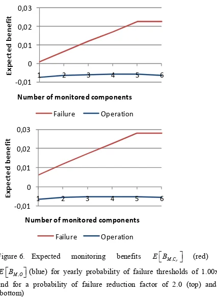
The calculated monitoring benefits are depicted in Figure 6 and Figure 7; the determined component sets are suppressed for simplicity. Two probabilities of failure reduction factors M

f p

∆ of 2.0 and 3.0 (top/bottom in Figure 6 and 7) and two yearly probability of failure thresholds of 1.00x10-3 and of 1.00x10-4 are considered (Figure 6 and Figure 7).

For both probabilities of failure thresholds and both probability of failure reduction factors the expected failure cost benefit (red lines) is positive for all number of monitored components. The higher the number of monitored components the higher failure cost benefit, i.e. the lower the risks associated to a structure with a monitoring system, until a maximum of monitored components.

-0,01 0 0,01 0,02 0,03

1 2 3 4 5 6

E x p e ct e d b e n e fi t

Number of monitored components

Failure Operation -0,01 0 0,01 0,02 0,03

1 2 3 4 5 6

E x p e ct e d b e n e fi t

Number of monitored components

[image:5.612.322.562.72.171.2]

Failure Operation

Figure 6. Expected monitoring benefits E B M C,F (red) and

, M O

E B_ _(blue) for yearly probability of failure thresholds of 1.00x10-3

and for a probability of failure reduction factor of 2.0 (top) and 3.0 (bottom)

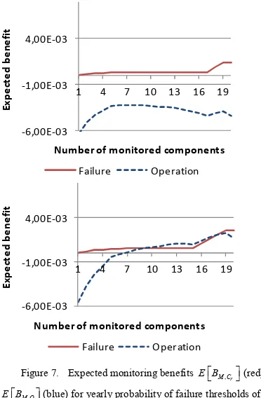
[image:5.612.326.539.339.630.2]

benefit is negative with minor dependency on the number of monitored components. For a yearly probability of failure thresholds of 1.00x10-4 the benefit becomes positive with 7 monitored components and the probability of failure reduction factor of 3.0. The expected benefit is then increasing until a number of 19 monitored components. It turns out that 19 hot spots of the support structure are subjected to the risk based inspection, i.e. that 19 hot spots have to be inspected during the service life of the structure.

-6,00E-03 -1,00E-03 4,00E-03

1 4 7 10 13 16 19

E

x

p

e

ct

e

d

b

e

n

e

fi

t

Number of monitored components

Failure Operation

-6,00E-03 -1,00E-03 4,00E-03

1 4 7 10 13 16 19

E

x

p

e

ct

e

d

b

e

n

e

fi

t

Number of monitored components

[image:6.612.67.253.145.429.2]

Failure Operation

Figure 7. Expected monitoring benefits _, F M C

E B_ _(red) and

, M O

E B_ _(blue) for yearly probability of failure thresholds of 1.00x10-4

and for a probability of failure reduction factor of 2.0 (top) and 3.0 (bottom)

IV. SUMMARY AND CONCLUSIONS

This paper contains actual research results in the field of condition monitoring support for the operation of offshore wind turbines. Both the machinery operation and the structural integrity management are addressed. It can be concluded that monitoring systems can support the operation management by reducing costs and risks.

For the machinery operation it is shown that CBM has significant cost advantages for the expected offshore failure rates. Clearly, cost-effective CBM requires a reliable monitoring system, and the CM information must be utilised by O&M planners to reduce MTTR and plan spares procurement in an efficient manner. The structural integrity management of the support structure can be supported by efficient monitoring systems building upon a condition based inspection and maintenance approach. On the basis of Multibrid M5000 wind turbine structure, it is shown under which conditions a risk reduction and an expected cost reduction or both can be achieved.

This paper is seen as the first step in developing holistic monitoring systems and approaches for the support of the operation management of offshore wind turbines.

V. REFERENCES

[1] EWEA, "The European offshore wind industry key trends and statistics 2010", 2011.

[2] EWEA. "The European offshore wind industry – Key trends and statistics: 1st half 2011". 2011 July 2011; Available from:

http://www.ewea.org/fileadmin/ewea_documents/documents/00_POLI CY_document/Offshore_Statistics/20112707OffshoreStats.pdf. [3] Ernst&Young, "Cost of and financial support for offshore wind", in A

report for the Department of Energy and Climate Change2009, DECC. [4] van Bussel, G.J.W. and M.B. Zaaijer, "Reliability, Availability and

Maintenance aspects of large-scale offshore wind farms, a concepts study.", 2001, Delft University of Technology: Delft.

[5] McMillan, D. and G.W. Ault, "Condition monitoring benefit for onshore wind turbines: sensitivity to operational parameters". IET Renewable Power Generation, 2008. 2(1): p. 60 - 72

[6] McMillan, D. and G.W. Ault, "Techno-Economic Comparison of Operational Aspects for Direct Drive and Gearbox-Driven Wind Turbines". IEEE Transactions on Energy Conversion, 2010. 25(1): p. 191 - 198

[7] Besnard, F. and L. Bertling, "An Approach for Condition-Based Maintenance Optimization Applied to Wind Turbine Blades". IEEE Transactions on Sustainable Energy, 2010. 1(2): p. 77 - 83 [8] Byon, E., L. Ntaimo, and Y. Ding, "Optimal Maintenance Strategies

for Wind Turbine Systems Under Stochastic Weather Conditions". IEEE Transactions on Reliability, 2010. 59(2): p. 393 - 404 [9] Guevara Carazas, F.J. and G.F. Martha de Souza, "Availability

Analysis of Gas Turbines Used in Power Plants". International Journal of Thermodynamics, 2009. 12(1).

[10] Hill, D., et al., "Application of statistical wind models for system impacts", in 44th International Universities Power Engineering Conference (UPEC)2010. p. 1-5.

[11] Dinwoodie, I. and D. McMillan, "Analysis Of Offshore Wind Turbine Operation & Maintenance Using A Novel Time Domain Meteo-ocean Modeling Approach", in ASME Turbo Expo 2012: Copenhagen, Denmark.

[12] BSH, "Konstruktive Ausführung von Offshore-Windenergieanlagen", in Bundesamt für Seeschifffahrt und Hydrographie (BSH) Nr. 70052007.

[13] GL Wind, "Richtlinie für die Zertifizierung von Condition Monitoring Systemen für Windenergieanlagen", 2007, GL Wind.

[14] Straub, D., "Generic Approaches to Risk Based Inspection Planning for Steel Structures", in IBK Bericht 2842004, ETH Zürich: Zürich. [15] JCSS, Probabilistic Assessment of Existing Structures. A publication

of the Joint Committee on Structural Safety2001: RILEM Publications S.A.R.L.

[16] Lind, N.C., "Reliability-based structural codes. Optimization theory; Reliability-based structural codes. Practical calibration; Safety level decisions and socio-economic optimization", in Safety of Structures under Dynamic Loading1978: Trondheim. p. 135-175.

[17] Straub, D., "Generic Approaches to Risk Based Inspection Planning for Steel Structures". PhD. thesis, 2004. Chair of Risk and Safety, Institute of Structural Engineering, ETH Zürich

[18] JCSS, "Probabilistic Model Code", 2006, JCSS Joint Committee on Structural Safety.

[19] Thöns, S., "Monitoring Based Condition Assessment of Offshore Wind Turbine Structures". PhD thesis, 2011. Chair of Risk and Safety, Institute of Structural Engineering, ETH Zurich

[20] Thöns, S., M.H. Faber, and W. Rücker. "Support Structure Reliability of Offshore Wind Turbines Utilizing an Adaptive Response Surface Method". in 29th International Conference on Ocean, Offshore and Arctic Engineering (OMAE 2010). 2010.