ANN vs. SVM : which one performs better in classification of MCCs in mammogram imaging



_Abstract

Classification of microcalcification clusters from mammograms plays essential roles in computer-aided diagnosis for

early detection of breast cancer, where support vector machine (SVM) and artificial neural network (ANN) are two

commonly used techniques. Although some work suggest that SVM performs better than ANN, the average accuracy

achieved is only around 80% in terms of the area under the receiver operating characteristic curve A

z

. This performance

may become much worse when the training samples are imbalanced. As a result, a new strategy namely balanced

learning with optimized decision making is proposed to enable effective learning from imbalanced samples, which is

further employed to evaluate the performance of ANN and SVM in this context. When the proposed learning strategy is

applied to individual classifiers, the results on the DDSM database have demonstrated that the performance from both

ANN and SVM has been significantly improved. Although ANN outperforms SVM when balanced learning is absent,

the performance from the two classifiers becomes very comparable when both balanced learning and optimized

decision making are employed. Consequently, an average improvement of more than 10% in the measurements of F1

score and Az measurement are achieved for the two classifiers. This has fully validated the effectiveness of our

proposed method for the successful classification of clustered microcalcifications.

Index Terms

—microcalification clusters (MCC), balanced learning, optimized decision making, neural

network, support vector machine, mammography, computer-aided diagnosis.

Corresponding Author: Dr. Jinchang REN

Centre for excellence in Signal and Image Processing Dept. of Electronic and Electrical Engineering University of Strathclyde

Glasgow, G1 1XW United Kingdom

Email: [email protected] Tel: +44-141-5482384

I. INTRODUCTION

Nowadays, breast cancer is the most common diagnosed cancer among woman. In the United States, about 182500 cases were diagnosed in 2008, and nearly 40500 women die from this disease annually [1]. In the United Kingdom, every year there are about 45000 cases are diagnosed, and more than 1100 women die from this cancer every month [3]. Since the reasons behind are still uncertain, early detection and diagnosis is the key for improving breast cancer prognosis [5, 6]. Among many available techniques, x-ray mammogram has been one of the most reliable methods for early detection of such disease [15]. Generally, it can increase the survival ratio by 20% to about 80% for patients. In England alone, around 1400 lives are saved each year via the NHS breast screening [3]. Other popular means for breast cancer detection include magnetic resonance imaging (MRI) [39], electrical impedance spectroscopy (EIS) [24], ultrasound [22], and infrared imaging [40].

Although mammogram contains useful information for the early detection of breast cancer, it is difficult for radiologists to make accurate and consistent judgments due to the huge amount of data and widespread screening. Consequently, about 10-30% cases are missed during the routine check [5]. With the assistance of computer-aided diagnosis (CAD), the overall sensitivity from human observers can be improved by 10% on average, which provides a promising solution in such a context.

In general, detection and classification of microclacification clusters (MCCs) from mammograms plays important roles in early diagnosis of breast cancer. In early detected cases, MCCs can be found in 30-50% of the screened mammograms. This will increase to 60-80% if histological examinations of cancer cases are considered. The difficulty for the detection of MCCs is due to i) small size but various shapes, ii) low contrast and unclear boundary from surrounding normal tissue, etc. [5, 33].

To solve such problems, a typical CAD system contains at least four stages including preprocessing, feature-based extraction of regions of interest (ROI), detection of MCCs, and classification. The preprocessing covers noise suppression and contrast enhancement, including histogram equalization etc. [30], which is useful for robust extraction of features and ROIs. The features include local statistics and texture modeling [13], wavelets [18, 31, 33, 34], and morphological features [23]. From the segmented ROIs, MCCs can be detected using heuristics [33], fuzzy sets [7, 15], sub-image decomposition and filtering [27], and machine learning algorithms [2, 32, 43], where shape features such as linear structure is widely used [12, 27, 46, 47].

by SVM is only 0.85 in comparison with 0.80 from ANN, which apparently has space for further improvement.

The reasons for the classification accuracy in terms of

A

_z above is not only the complexity of the problem, i.e. containing cases that cannot be judged even by radiologists as analyzed in [44], but also the difficulty in dealing with imbalanced training set in machine learning. The imbalance here refers to the fact that one class is more heavily represented than the other. This is a common problem in real-world domains in detecting rare but important cases from large suspiciously normal samples [19]. Most existing machine learning algorithms fail in dealing with imbalanced data set as their predictions are biased to the class of majority samples [20]. To solve such problems, an improved over-sampling based balanced learning strategy is proposed in this paper and the performances from SVM and ANN are evaluated in classification of MCCs. Along with the proposed optimized decision making, it is found that the classification rate of both ANN and SVM has been significantly improved. The proposed method is found effective in improving both the sensitivity and specificity rate while maintaining the computing complexity of the classifier. The remaining part of this paper is organised as follows. Section II contains introductory concepts related to the SVM and ANN classifiers. In Section III, the proposed balanced learning and optimized decision making is presented. Section IV discusses the evaluation criteria and implementation details including the data set and extracted features. Experimental results are given and analyzed in Section V to fully validate the proposed methodology. Finally, brief conclusions are drawn in Section VI.

II. REVIEW OF SVM AND ANNLEARNING TECHNIQUES

In this paper, the classification of MCCs is treated as a two-class pattern classification problem, and the two classes are referred to as “malignant” and “benign”. If we denote





d

x

as an input vector or pattern to be classified, and let scalar

y

denote its

class label, i.e.

y



{



1

,

1

}

for SVM and

y



{

0

,

1

}

for ANN. The training set

L

contains

M

samples, i.e.

L



{(

x

_i

,

y

_i

)}

and

i



[

1

,

M

]

. The problem here is how to determine a classifier

f

(

x

)

which can make correct decision and classify the input pattern into suitable classes. In this section, brief introductions to SVM and ANN are presented, which forms the base of our proposed improved classifier as presented in the next section.

A. The SVM Classifier

In general, a SVM classifier can be formed as follows,

b

f

_SVM

(

x

)



w

T



(

x

)



(1)

where parameters

w

and

b

respectively denote a weight vector and a bias that can be determined in the training process through minimizing the cost function below, and



(



)

refers to a nonlinear mapping to map the input vector

x

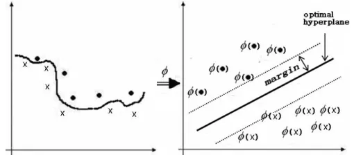
into a higher dimensional space for easily separated by a linear hyperplane as illustrated in Fig. 1.

]

,

1

[

K

k



,

{

s

_k

}



L

is a small subset of the training set. Hence, the SVM function becomes

















_

)

(

)

(

)

,

(

)

,

(

)

(

T 1 k k K k k SVM

K

b

K

f

s

x

s

x

s

x

x





(2)

[image:4.612.178.433.178.290.2]

where

K

(



,



)

is denoted as a kernel function to represent the effect of the nonlinear mapping



(



)

in classification.

Figure 1. Illustration the concept of SVM to map a nonlinear problem to a linear separable one.

Some common used kernel functions are summarized below, including linear and two nonlinear functions. If the training samples are not linear separable, non-linear kernel functions are better choice. In addition, the associated parameters

p

and



are determined automatically during the training process.

1) Linear kernel

K

(

x

_i

,

x

_j

)



x

T_i

x

_j

2) Polynomial kernel

K

(

x

_i

,

x

_j

)



(

x

_iT

x

_j



1

)

p

3) RBF kernel

(

,

)

,

(

2

2

)

1

2

 







 i j





e

K

x

_i

x

_j x x

B. The ANN Classifier

Generally speaking, ANN can be considered as an information processing system which is composed of a network of interconnected simple processing elements, i.e. neurons. Determined by the connections between these neurons and the associated parameters, ANN can exhibit complex global behavior to generate expected outputs via supervised or unsupervised learning. Inspired by the biological nervous system, the learning process is to adjust the connection strength or weights between the neurons. Each neuron forms a node in the whole network and after training each node is assigned with a determined bias or threshold. For each interconnection between two nodes, a weight is also assigned to represent the link-strength between the neurons.

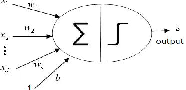
Let

x



(

x

₁

,

x

₂

,...,

x

d

)

T be an input vector and

T 2

1

,

,...,

)

(

w

w

w

d



w

the weight vector, the output of a single neuron

z

)

(

)

(

1 T













d

i

w

i

x

i

b

g

b

g

z

w

x

(3)

where

g

(



)

is namely an activation function to decide whether the perceptron should fire or not. The sigmoid function 1

)

1

(

)

(

x





e

x 

Sig

is the most popular used activation function, others include tanh and step functions, etc.

Figure 2. Illustration the effect of a single neuron.

Using the same process as to determine the output of a single neuron, the output of the whole network can be also calculated in a topological manner. This means that for each neuron its inputs from other neurons need to be computed before determining its output. As seen, the weight vector and the bias associated to each connection and each node will influence the outputted results, and they can be determined in training or learning process as follows. First of all, the topology of the ANN needs to be specified, and feed-forward ANN is adopted as it has been widely applied for the classification of MCCs [8, 23, 32, 41]. A feed-forward ANN is a multi-layer perceptron (MLP) which contains three or more layers of neurons, i.e. one input layer, one output layer and at least one hidden layer. With a given training set, a specified activation function and a learning ratio



where





(

0

,

1

)

, the learning process for supervised training using the well-known back-propagation algorithm can be described in the following three stages.

Firstly, the initial weights and bias are set randomly between

[



1

,

1

]

to attain a group of outputs

z

(t) at

t



1

referring to

the first round of iteration. Then, an error function is decided as

(

)

(

)

/

2

1 2 ) (









M i t i i

z

y

t



using the sum squared error between

the estimated output

z

and the target output

y

. Finally, the error signal at the output units is propagated backwards through the whole network to update the weights using the gradient descent rule

ij ij

w

t

t

w











(

)





(

)

(4)

where

w

_ij refers to a weight between the

j

th node in a given layer and the

i

th node in the following layer. With updated weights,

we can set

t



t



1

to start a new iteration until the network becomes convergence. This can be measured by using a small change ratio of



(



)

or a given number of iterations.

C. Comparisons between SVM and ANN

[image:5.612.214.400.157.247.2]

difference is mainly on how non-linear data is classified. Basically, SVM utilizes nonlinear mapping to make the data linear separable, hence the kernel function is the key. However, ANN employs multi-layer connection and various activation functions to deal with nonlinear problems. In fact, single layer ANN can only generates linear boundary, and the 2nd layer can combine the linear boundary together; while at least three layers are required to produce boundary of arbitrary shapes.

Using the gradient descent learning algorithm, ANN intends to converge to local minima. As a result, it suffers from the over-fitting problem. On the other hand, SVM tends to find a global solution during the training as the model complexity has been taken into consideration as a structural risk in SVM training. In other words, ANN minimizes only the empirical risk learnt from the training samples, but SVM considers both this risk and the structural risk. Consequently, the training results from SVM have better generalization capability than those from ANN. Therefore, SVM and ANN are two typical classifiers which are used to validate our balanced learning strategy as discussed in the next sections.

III. BALANCED LEARNING WITH OPTIMIZED DECISION MAKING

Despite the good generalization capability of SVM achieved for pattern recognition, the accuracy in classifying MCCs remains unsatisfied at around 80% in terms of

A

_zmeasurement [10, 29, 42, 44]. This accuracy may further degrade if the distribution of the samples is severely imbalanced [44]. Unfortunately, such imbalanced distribution is widely found for MCCs classification, as usually there are much more (>4 times) benign samples than malignant ones in the training sets [44, 46]. Therefore, the performance of the classifier may bias to the majority class and fails for correct detection of MCCs. To overcome such drawbacks, an improved strategy namely balanced learning is proposed and presented as follows.

A. Strategy in Balanced Learning

There are two main technical streams to achieve balanced learning, including data level and algorithm level methods [25, 26, 49]. At the data level, the former refer to many re-sampling solutions to balance the training data [4]. On the other hand, algorithm level solutions intend to adjust the cost function, decision threshold or the learnt probability for refined learning, such as the work reported in [19-20, 35]. Using Bayes optimal classifier theory, it is found that individual classifier has a fundamental performance limit which makes it little better than that of the majority class [4, 9, 25]. Consequently, data-level solutions are preferred for balanced training in our paper.

As random over-sampling may increase the likelihood of over-fitting in dealing with the duplicated samples, several smart sampling techniques have been presented such as synthetic over-sampling (SMOTE) [4]. In SMOTE, synthetic minority samples are generated via interpolation of one random sample and its nearest neighbors. Some other smart sampling techniques include one-sided selection, cluster-based over- sampling and Wilson’s editing etc., and details of which can be referred to the work in [21].

B. Proposed Balanced Learning Strategy

In fact, random sampling and smart sampling have both been used in learning techniques. According to the extensive experiments in [21], it is found that random sampling outperforms several smart sampling techniques and unaltered data set. However, the evaluation in [44] indicates that random over-sampling seems not improving the performance in classification of MCCs, and similar finding is concluded in detecting sentence boundaries in [26]. Besides, it is indicated that SMOTE may outperform down-sampling in certain cases [26]. These inconsistent results need to be further clarified before applying any sampling strategies to classify MCCs for improved performance.

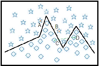
[image:7.612.225.388.496.604.2]

A typical two-class classification problem is illustrated in Fig. 3, where contains combined linear decision boundaries. This is very common in machine learning domain and the segment of the decision boundary can also be nonlinear. For the two classes marked as circle and star shapes, two pairs of same-class samples are extracted satisfying minimum neighboring distance and marked as A-B and C-D. According to the rules of smart sampling in SMOTE, synthetic samples can be generated for balanced learning. Unfortunately, the generated samples in these cases are unreliable noisy ones which may inevitably degrade the performance of training and classification. The more complex the decision boundary is, the more noisy samples may be introduced via smart sampling, and hence the worse performance may be achieved. On the other hand, smart sampling like SMOTE may work well in simpler cases such as the linear problem in detection of sentence boundary in [26].

Figure 3. Illustrating a two-class problem with combined linear decision boundaries where the interpolation using SMOTE may fail for the sample pairs of A-B and C-D.

normalizing the range of the feature values within [-1,1]) to one item of the feature values which is randomly determined. This helps to keep consistency between generated samples and the original ones for balanced learning and avoiding the problem caused by smart sampling as discussed above. Please note that it is assumed that the samples in our test set contain no noise instances thus the over-fitting caused by over-sampling in training can be avoided.

C. Criteria for Optimized Decision Making

In a more general case, classifiers like ANN and SVM produce predicted outputs in continuous real values rather than binary symbols. Conventional methods use simple thresholding in decision making. If the output is larger than a chosen threshold, say 0 for SVM and 0.5 for ANN, a positive sample is detected. Otherwise, the sample is decided as negative. However, this simple thresholding suffers imbalanced distribution of the training outputs and leads to poor performance. To solve such problems, on the contrary, optimized decision making using optimal thresholding is proposed and described as follows.

The proposed optimal thresholding is achieved through statistical analysis of the outputs of the classifiers, where SVM is taken to show its principles. For a given input sample

x

_i, let

y

_i be a target label where

y

i



{



1

,

1

}

. Also let

z

i denote the

predicted output satisfying

z

_i



(

a

₀

,

a

₁

)

and the parameters

a

₀ and

a

₁ represent respectively the lowest and the highest

boundary of the output from the classifier. Then, two conditional probabilities

p

(

z

_i

|

y

_i



1

)

and

p

(

z

_i

|

y

_i





1

)

are obtained

from the initial classification. For a given threshold

T



(

a

0

,

a

1

)

, the sum of error classification rate

Err

is determined as























  

i i i i

i i i i

T

z

y

z

p

err

T

z

y

z

p

err

err

w

err

w

T

Err

)

,

1

|

(

)

,

1

|

(

)

(

1 1 1 1 1 1 (5)

where the weights

w

₁ and

w

_1 are simply set as ½. Then, an optimal threshold

T

_svm can be determined when the minimum cost of error classification is achieved, i.e.

T

_,

arg

min

(

Err

(

T

))

T accu

svm



(6)

Similarly, an optimal threshold

T

_ANN,_accu can also be determined for the ANN classifier via statistical analysis of its outputs.

)

/(

TP

FN

TP

Recall





(7)

)

/(

TP

FP

TP

Precision





(8)

Precision

Recall

Precision

Recall

F





2

*

1 (9)

where the

F

₁ score is utilized to enable a single measure of performance.

Using the

F

₁ score measurement, another group of thresholds can also be determined by maximizing the

F

₁ score in the training set whilst adjusting the threshold below. Please note the range of the threshold value is determined between the minimum and the maximum outputted values of the classifiers.

)

_

_

_

(

max

arg

)

_

_

_

(

max

arg

1 _ 1 , 1 _ 1 ,

t

under

F

N

TrainingAN

T

t

under

F

M

TrainingSV

T

t threshold F ANN t threshold F svm





(10)

When receiver operating characteristic (ROC) curve is plotted for quantitative evaluations of classifiers, especially for the detection and classification of MCCs [5], another important measurement

Az

can be determined as the area under the ROC curve. Consequently,

Az

is also used as an important evaluation criterion [5], where

Az



1

indicates an ideal case with

%

100



rate

TP

and

FP

_rate



0

. By maximizing the

Az

measurement of the classifiers, another group of optimal thresholds

can also be determined in a similar way as defined in (10)

)

_

_

_

(

max

arg

)

_

_

_

(

max

arg

_ 1 , _ 1 ,

t

under

A

N

TrainingAN

T

t

under

A

M

TrainingSV

T

z t threshold F ANN z t threshold F svm





(11)

When the determined optimal threshold, say

T

_svm,F1, is applied for testing, it will be used to make a decision in classifying testing samples into negative and positive classes. Ideally, we would expect that this threshold can also help to achieve the maximum

F

₁ score in the testing set if the corresponding class of each test sample can also be labeled. Unfortunately, this is not always true due to the sample distribution difference between the training set and the testing set. Therefore, the optimal threshold for the testing set can be extracted and denoted as

Test

_svm,F1. Then, the inconsistency of the two optimal thresholds is measured by

(

,

)

|

|

0

1 , 1 , 1 , 1









F SVM F SVM F SVM

T

Test

T

F

SVM

(12)

Apparently, a smaller



(

SVM

,

F

₁

)

indicates a more consistent measurement of the thresholds extracted for the training and testing set, and vice versa. Similarly, we can also extract such inconsistency measurements for other thresholds hence we will have

)

,

(

SVM

Accu

decision making and how consistency different criteria are in such a context has been fully validated using the improved results as presented in Section V.

IV. DATA SET AND IMPLEMENTATION

To validate the proposed learning strategy, quantitative evaluations are achieved using a large data set extracted from the well-known DDSM database. The data set and feature set as well as evaluation strategy are discussed in this section, along with some implementation details. These are essential for consistent evaluation of our proposed methodology to compare with others.

A. Data Collection

Suspicious MCC regions are detected through optimal filtering using texture measurements [45-46]. Firstly, some pre- processing is applied to remove the influence of background and several artefacts like white/black spots and scratches. Then, optimal filtering is employed using local frequencies in terms of energy distribution extracted from mammograms. Finally, adaptive thresholding is utilized as post-processing for further robustness. Relevant details can be found in [45].

To verify the effectiveness of the proposed approach over ANN and SVM classifiers, in total 748 suspicious MCCs are collected, which contain 633 benign and 115 malignant samples where the ratio between them is over 5.5. These MCCs are extracted from 295 full-field mammograms in the well-known DDSM database, where the mammography data from more than 2600 patients are scanned at 50 microns using LUMISYS [16-17]. The collected MCCs are then randomly divided into two dataset for training and testing purposes, receptively, and the final performance is evaluated using cross validation.

In our experiments, all 748 MCC samples are randomly partitioned into two subsets for training and test, respectively. All the positive samples in the training set are over-sampled to enable balanced learning using SVM and ANN. The models determined are then used to classify samples in the test set. This process is repeated 10 times to overcome any bias in data partition. The average performance over these 10 times is taken as a final result for evaluations. Please note the over-sampling of positive samples is only applied to the training set and the test set remaining imbalanced. This is because we assume that there is no prior information to indicate the class each sample belongs to, which consequently enables blind test where balanced learning followed by testing with imbalanced data is used.

B. Feature Descriptions

Generally speaking, breast microcalcifications appear as small white specks in various patterns on the mammogram [5]. Whether their clusters are malignant or benign depends on the size, shape and geographic distribution of all microcalcification regions in a cluster. For example, suspicious MCC samples tend to be tightly clustered and have certain linear structure, etc. Therefore, the extracted features need to measure these properties accordingly which include the area, the scattered degree and brightness of the regions in the cluster.

As seen, except the first three single measures, the other 20 features in the feature set are composed of the mean and standard deviation values of ten measures. In addition, these 20 features can be categorized into three classes including i) intensity statistics (#4-#5), ii) shape features (#6-#17), and iii) linear structure features (#18-#23). Introductions to most of these features can be found in [2, 5, 12, 23, 28-30, 38, 46].

Due to the fact that about 80% of the diagnosed breast cancer cases are for women over 50 years old [3], age is a good indicator and has been widely used in the classification of MCCs [5, 23, 46]. A MCC is defined as a group of at least three microcalcifications within 1 cm2, and the number of microcalcifications in a cluster is also an important feature [23, 30, 42, 46]. The mean of the least distance of all regions in a cluster refers to the average value of inter-distance between each region and its neighboring ones [42], which can be also used to measure the scattered degree of the distribution of the microcalcifications in a cluster. In addition, the intensity measures are also useful as high intensity is expected for the white specks in MCCs [5, 29].

Table 1. List of features used for the classification of MCCs where std. means standard deviation.

Index Notes Descriptions

#1 Age of the patient [5, 23, 46]

#2 Number of regions in a cluster [[23, 30, 42, 46].

#3 mean Minimum inter-distance of all regions in a cluster [42]

#4 mean

Average intensities of all regions in a cluster [5, 29] #5 std.

#6 mean

Areas of all regions in a cluster [5, 23, 29, 30, 46] #7 std.

#8 mean

Compactness of all regions in a cluster #9 std.

#10 mean

Fourier description of all regions in a cluster #11 std.

#12 mean

Moment-based measure of all regions in a cluster #13 std.

#14 mean

Eccentricity of all regions in a cluster #15 std.

#16 mean

Spread of all regions in a cluster #17 std.

#18 mean

Average minimum std. of

r

(



,

l

)

of all regions in a cluster [12, 27, 46, 47] #19 std.

#20 mean

Average std. of the minimum std. of

r

(



,

l

)

at various directions in all regions in a cluster #21 std.

#22 mean

Average std. of the string of length

l

, starting from each point in a region at direction



#23 std.

Shape features are also commonly utilized important indicators in this field, which include the area (size), the compactness, Fourier descriptors, moments, eccentricity, and the spread. The definitions of these shape features can be referred to [5, 23, 29-30, 46]. Please note that these measures can be extracted from each microclacification region within a candidate MCC, and the mean and standard derivation values over all regions are then determined for classification purpose.

direction, which can be denoted as

r

(



,

l

)

where



and

l

refer respectively to the direction and the length in the linear structure. In addition, the pixel intensities on the line are higher than that of their surrounding pixels, and also the length of the line should be larger than its width. To measure the consistency of the intensities along the linear structures in a MCC, six features are extracted as summarized in Table 1 using the mean and standard deviation values of three measurements [46].

C. Optimizing Classifiers

For the ANN classifier, the number of nodes in the hidden layer is empirically set as 15 for the better results achieved. The training process stops when the training performance keeps unchanged over a long time, say more than 4000 iterations. The performance is measured using the

F

₁, and the parameters which yield the highest

F

₁ value is stored and used for testing. In addition, the RBF kernel has been adopted in our SVM implementation as it can generate particular good results. The other important parameters for the SVM classifier include



of the Gaussian kernel and soft margin parameter

C

. These are determined via cross validation by selecting various combinations of the parameters values. Finally, the parameter group which yields the maximum overall accuracy is chosen as the optimal one.

In our evaluation,

Recall

vs.

Precision

rates are plotted for ROC analysis. For each pair of these two rates, one sample point is obtained. When the threshold for decision making varies, as described in section III(C), the recall and precision rates are updated. As a result, a group of recall vs. precision rate pairs is produced to form a plot of the ROC curve. The plotted curve can then be used to evaluate the performance of the classifier, and detailed evaluations are presented in the next section.

V. RESULTS AND DISCUSSIONS

In this section, comprehensive experimental results from ANN and SVM classifiers are presented for the classification of benign and malignant MCCs. Quantitative evaluations are used to validate the effectiveness of our proposed method including balanced learning and optimal decision making. In addition, it is worth noting that in [36]

Az

is approximated as the average of the recall rate and the overall accuracy. In this paper, a more accurate calculation of the

Az

based on its definition is utilized.

A. Performance of Balanced Learning

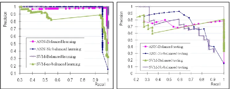
First of all, the performance of balanced learning is compared with those training with the original data, and we set the training ratio as 80%, i.e. 80% of the samples for training and 20% for testing. The ROC curves are plotted in Fig. 4 to show the performances in training and testing of SVM and ANN with or without balanced learning, respectively, where several facts can be summarized as follows.

performance of the two classifiers becomes quite comparable. This no doubt has confirmed that balanced learning helps to yield to improve the classifier. Regarding training, it has generated significant higher recall rate for SVM and slightly higher recall rate for ANN though its recall rate without balanced learning is already high enough. For testing, balanced learning produces much improved results for both ANN and SVM.

Finally, please note that the plotted ROC curves are based on varying the threshold value to obtain the corresponding recall-precision pairs. When the threshold is too small, all samples may appear above this threshold hence no positive samples are missed. This corresponds to a recall rate of 1 but the precision rate can be very small due to a large amount of false positives are detected. When the threshold increases but still below a certain level, the recall rate remains yet the precision rate increase as well. This explains the short vertical line segments in the plotted curve in Fig. 4. On the other hand, a very high threshold will generate a precision rate of 1, i.e. no false positives detected. However, the recall rate turns to be small due to missing detection of the majority of positive samples. When the threshold decreases, the precision rate may remain unchanged but the recall rate increases. This will inevitably generates horizontal line segments in the ROC curves.

[image:13.612.121.492.335.479.2]

Figure 4. ROC curves of training and testing performances from SVM and ANN with or without balanced learning.

Quantitative comparisons of the results from ANN and SVM are respectively reported in Table 2 and Table 3, and no optimized decision making is utilized in the testing. From these two tables, several facts can be extracted as follows:

 When balanced learning is absent, as shown in Table 2, ANN outperforms SVM in both training and testing. For training,

the

F

₁ score of 0.979 and

Az

measurement of 0.981 from ANN are much bigger than those from SVM at 0.796 and 0.841, respectively, which refers to a significant superior performance. However, this significance is degraded in the testing results, though ANN still generates slightly better results than SVM.

 With balanced learning in Table 3, the training results from the two classifiers are quite close to each other. However, ANN yields much better results than SVM in the testing set.

two classifiers, especially for the SVM which performs much worse in Table 2. It contributes SVM about 9% in

F

₁

score and 12% in

Az

measurement for testing, yet 14-20% gain for training. On the other hand, even the performance is quite good in Table 2, balanced learning still helps to improve the performance of ANN, especially for testing, where the improvements for

F

₁ score and

Az

measurement are about 13% and 12%, respectively.

Table 2. Training and testing results without balanced learning.

Training Testing

ANN SVM ANN SVM

Recall

0.960 0.968 0.728 0.779

Precision

1.000 0.677 0.697 0.610

1

F

0.979 0.796 0.712 0.684

Az

0.986 0.841 0.780 0.718

Table 3. Training and testing results with balanced learning.

Training Testing

ANN SVM ANN SVM

Recall

0.991 1.000 1.000 1.000

Precision

0.980 0.961 0.723 0.634

1

F

0.985 0.980 0.840 0.776

Az

0.990 0.983 0.905 0.837

In the following, we are going to further explain the observations above. Firstly, the high performance of ANN shown in these tables has indicated that ANN is capable of model the problem accurately. Although in training the

F

₁ score and

Az

value are

larger and closer to each other, much smaller

F

₁ values in testing are yielded. This is caused by lower

Precision

values caused by false positives. Due to the severe imbalanced data used for testing, a high overall accuracyis still achieved under these false positives to yield a higher

Az

measurement. In other words, the ratio between the number of false positives to the number of malignant samples is much larger than the ratio between it to the number of benign samples, and this has led to lower

F

₁ but higher

Az

values. In addition, the contributions of balanced learning to SVM can be found in two parts, i.e. much improved precision rate in training and improvements in both the

F

₁ score and

Az

measurement in testing. With a recall rate of 1 in both training and testing, balanced learning has led to accurate of positive samples in SVM. The relatively lower precision rate generates from SVM inevitably shows the weakness of SVM in modelling the diversely distributed negative samples.

B. Performance of Optimized Decision Making

with those in Table 2 and Table 3, we can clearly find several facts which are summarized as follows.

Without balanced learning, optimized decision making contributes for the ANN about 1% in

F

₁ and 2% in

Az

measurements, and this is mainly due to the much increased recall rate although the precision rate slightly degraded. For the SVM, the corresponded contributions are 2.4% in

F

₁ and 2.5% in

Az

and can be found to the two measurements, yet even degradation in

Az

, and this is caused by much degraded recall rate though the precision rate is improved.

When balanced learning is introduced, the improvements for ANN are 4.1% in

F

₁ and 2.5% in

Az

due to the 6.5% increase

of the precision rate. In addition, SVM gains 11.1% in

F

₁ and 10.1% in

Az

measurements with a dramatic 16.3% increase of the precision rate. Also it seems SVM slightly outperforms ANN in this group of results. This on one hand has fully validated the effectiveness of the proposed strategy for optimized decision making in terms of

Recall

,

Precision

,

F

₁

and

Az

measurements. On the other hand, significant improvements have achieved for the SVM classifier.

No matter balanced learning is used to not, optimized decision making improves the performance of ANN in

F

₁ and

Az

[image:15.612.173.419.507.599.2]

measurements. However, optimized decision making only works to SVM when balanced learning is used. The reason behind is that the linear classification boundary in SVM requires the sample data to be consistently distributed in training and testing set, yet this is hardly to be held when the samples are severely imbalanced. On the other hand, nonlinear decision boundary used in ANN is less affected by this assumption, and this is why optimized decision making improves the performance of ANN even without balanced learning. In other words, this shows that SVM needs more the proposed optimized decision making than ANN to reach a better classification.

Table 4. Testing results from ANN and SVM under optimized decision making with or without balanced learning.

No balanced learning Balanced learning

ANN SVM ANN SVM

Recall

0.819 0.750 1.000 1.000

Precision

0.644 0.671 0.788 0.797

1

F

0.721 0.708 0.881 0.887

Az

0.799 0.743 0.930 0.938

Please note the criterion of maximizing the

F

₁ score is adopted to generate the results in Table 4 for optimised decision

making. In the following, the performance of the three criteria, i.e. minimizing error, maximizing the

F

₁ score and maximizing the

simply because the threshold

T

_svm,. determined from the training set cannot be applied to estimate

Test

_svm,.for optimized decision

[image:16.612.178.419.204.283.2]

making in the testing set. When the balanced learning is employed, though the inconsistency of the thresholds for ANN is reduced which indicates an improved classification performance, significant reduction of such inconsistency can be found for the thresholds determined from SVM. Consequently, optimized decision making has considerable contributions to SVM and makes it even slightly outperform ANN in such a context.

Table 5. Inconsistency measurement of the optimal thresholds extracted from training and testing set.

No balanced learning Balanced learning

ANN SVM ANN SVM

)

(.,

Accu



4.3% 17.6% 1.7% 1.5%

)

(.,

F

1



4.4% 22.2% 1.6% 1.4%

)

(.,

A

_z



5.1% 25.7% 2.0% 1.7%

C. Performance under Various Training Ratios

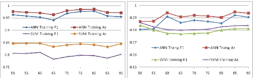
In this group of tests, the performance under various training ratios is compared. Under various training ratios, the training results and two groups of testing results with or without optimized decision making are evaluated in terms of

F

₁ and

Az

measurements. These results are illustrated in Fig. 5, Fig. 6 and Fig. 7, where Test2 denotes results when optimal decision making is utilized. In total there are four curves plotted in each plot, two for SVM and two for ANN, which forms two pairs. Each pair of the curves is plotted using the training ratio (changed from 50% to 90%) vs. performance of

F

₁ and

Az

measurements and they are further discussed as follows.

Figure 5. Training results from ANN and SVM using plots of training ratio (x-axis) vs.

F

₁ and

Az

measurements, where the left and the right plots refer respectively to results without or with balanced learning.

[image:16.612.105.513.466.592.2]

plotted curves than that of ANN, especially for the

F

₁ score, which indicates that SVM is less sensitive to the training ratios.

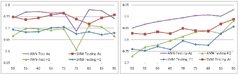
Figure 6. Testing results from ANN and SVM using plots of training ratio (x-axis) vs.

F

₁ and

Az

measurements without optimised decisionn making, where the left and the right plots refer respectively to results without or with balanced learning.

[image:17.612.105.516.95.224.2]

Fig. 6 shows the testing results from SVM and ANN without optimized decision making. Firstly, no matter balanced learning is used or not, both ANN and SVM produces higher

Az

values than the

F

₁ scores. Secondly, when balanced learning is absent, the results from the two classifiers appear quite sensitive to the traiing ratios, where SVM again outperforms ANN in such a context. Thirdly, when optimized decision making is employed, the testing results shows an ascent indication when the training ratio increases. Finally, ANN outperforms SVM in terms of the

F

₁ and

Az

measurements in most cases.

Figure 7. Testing results from ANN and SVM using plots of training ratio (x-axis) vs.

F

₁ and

Az

measurements with optimised decisionn making, where the left and the right plots refer respectively to results without or with balanced learning.

[image:17.612.101.513.423.553.2]

cases. Finally, the performance of SVM is less sensitive to the training ratios, though it yields smaller

Az

values than that of ANN when balanced learning is not used.

D. Computational Complexity

In comparison with conventional ANN and SVM, the proposed balanced learning and optimized decision making do need additional computations. Since the process of optimized decision making is not employed in the training iterations, it can be simply ignored. As discussed in [36], the additional computational burden from balanced learning is found to be

1

*

)

1

/(

2









K

K



(13)

where

K



2

is the rate of over-sampling of the minority class,





1

refers to a ratio of the number of iterations to converge the classifier when balanced learning is used in comparison to the number of iterations needed without balanced learning. This fast converging might due to the improved distributions of training samples from our balanced learning. When





0

.

7

,

)

1

/(

4

.

1

4

.

0









K

, indicating to a maximum of 40% additional computing burden, which is totally acceptable for the

benefit of much improved performance.

VI. CONCLUSIONS

In this paper, performance of ANN and SVM in classification of MCCs in mammogram imaging is evaluated, using large and imbalanced data from the well-known DDSM database. Balanced learning and optimized decision making are proposed in classifying MCCs into benign and malignant categories. In total 748 samples are employed in our experiments, and the main findings can be summarised as follows.

ACKNOWLEDGMENT

Firstly, we need thank anonymous reviewers and the editor for their constructive comments to further improve the quality of this paper. We would also like to thank Dr. Z.-Q. Wu for his helps in data collection and feature extraction in this work.

REFERENCES

1. American Cancer Society: Cancer facts and figures, http://www.cancer.org, 2009.

2. L. Bocchi, G. Coppini, J. Nori, G. Valli, “Detection of single and clustered microcalcifications in mammograms using fractals models and neural networks,”

Med. Eng. & Phy., 26(4) (2004) 303-312.

3. Cancer Research UK: Key Facts on Breast Cancer, http://info.cancerresearchuk.org/cancerstats/types/breast/, 2009.

4. N.V. Chawla, K.W. Bowyer,, L.O. Hall, W.P. Kegelmeyer, “SMOTE: synthetic minority over-sampling technique,” J. Artif. Intell. Res., 16 (2002) 321-357. 5. H.D. Cheng, X. Cai, X. Chen, L. Hu, X. Lou, “Computer-aided detection and classification of microcalcifications in mammograms: a survey,” Pattern Recog.,

36(12) (2003) 2967-2991.

6. H.D. Cheng, X.J. Shi, R. Min, L.M. Hu, X.P. Cai, H.N. Du, “Approaches for automated detection and classification of masses in mammograms,” Pattern Recog., 39(4) (2006) 646-668.

7. H.D. Cheng, J. Wang, X. Shi, “Microcalcification detection using fuzzy logic and scale space approaches,” Pattern Recog., 37(2) (2004) 363-375.

8. M. De Santo, M. Molinara, F. Tortorella, M. Vento, “Automatic classification of clustered microcalcifications by a multiple expert system,” Pattern Recog., 36(7) (2003) 1467-1477.

9. C. Drummond, R.C. Holte, “Severe class imbalance: why better algorithms aren’t the answer,” LNCS, vol. 3655, pp. 539-546, 2005.

10. I. El-Naqa, Y. Yang, N.P. Galatsanos, et al, “A similarity learning approach to content-based image retrieval: application to digital mammography,” IEEE Trans. Med. Imaging, 23(10) (2004) 1233-1244.

11. I. El-Naqa, Y. Yang, M.N. Wernick, et al., “A support vector machine approach for detection of microcalcifications,” IEEE Trans. Med. Imaging, 21(12) (2002) 1552-1563.

12. J. Ge, B. Sahiner, L.M. Hadjiiski, H.-P. Chan, J. Wei, M.A. Helvie, C. Zhou, “Computer aided detection of clusters of microcalcifications on full field digital

mammograms,” Med. Phys., 33(8) (2006) 2975-2988.

13. J. Grim, P. Somol, M. Haindl, J. Danes, “Computer-aided evaluation of screening mammograms based on local texture models,” IEEE Trans. Image Proc., 18(4) (2009) 765-773.

14. L. Hadjiiski, B. Sahiner, H.-P. Chan, et al, “Classification of malignant and benign masses based on hybrid ART2LDA approach,” IEEE Trans. Med. Imaging, 18(12) (1999) 1178-1187.

15. A.E. Hassanien, “Fuzzy rough sets hybrid scheme for breast cancer detection,” Image and Vision Comput., 25(2) (2007) 172-183.

16. M. Heath, K. Bowyer, D. Kopans, W.P. Kegelmeyer, R. Moore, K. Chang, S. MunishKumaran, “Current status of the digital database for screening

mammography,” in Proc. the 4th Int. Workshop on Digital Mammography, pp. 457-460, 1998.

17. M. Heath, K. Bowyer, D. Kopans, R. Moore, W.P. Kegelmeyer, “The digital database for screening mammography,” in Proc. the 5th _{Int. Workshop on}

Digital Mammography, pp. 212-218, 2001.

19. X. Hong, S. Chen, C. Harris, “A kernel-based two-class classifier for imbalanced data sets,” IEEE Trans. Neural Netw., 18(1) (2007) 28-42.

20.K. Huang, H. Yang, I. King, M.R. Lyu, “Maximizing sensitivity in medical diagnosis using biased minimax probability machine,”IEEE Trans. Biomed. Eng.,

53(5) (2006) 821–831.

21.J.V. Hulse, T.M. Khoshgoftaar, A. Napolitano, “Experimental perspectives on learning from imbalanced data,” in Proc. 24th _{Int. Conf. Machine Learning}

(ICML), vol. 227, pp. 935-942, 2007.

22. S. Joo, Y.S. Yang, W.K. Moon, H.C. Kim, “Computer-aided diagnosis of solid breast nodules: use of an artificial neural network based on multiple

sonographic features,” IEEE Trans. Med. Imaging, 23(10) (2004) 1292-1300.

23. M. Kallergi, “Computer-aided diagnosis of mammographic microcalcification clusters,” Med. Phys., 31(2) (2004) 314-326.

24. T.E. Kerner, K.D. Paulsen, A. Hartov, S.K. Soho, S.P. Poplack, “Electrical impedance spectroscopy of the breast: clinical imaging results in 26 subjects,” IEEE Trans. Med. Imaging, 21(6) (2002) 638-645.

25. S. Kotsiantis, D. Kanellopoulos, P. Pintelas, “Handling imbalanced datasets: a review,” GESTS Int. Trans. Computer Science and Eng., 30(1) (2006) 25-36. 26. Y. Liu, N.V. Chawla, M.P. Harper, E. Shriberg, A. Stolcke, “A study in machine learning from imbalanced data for sentence boundary detection in speech,”

Computer Speech Language, 20(4) (2006) 468-494.

27. R. Nakayama, Y. Uchiyama, K. Yamamoto, et al, “Computer- aided diagnosis scheme using a filter bank for detection of microcalcification clusters in

mammograms,” IEEE Trans. Biomed. Eng., 53(2) (2006) 273-283.

28. M. Nemoto, A. Shimizu, Y. Hagihara, et al, “Improvement of tumor detection performance in mammograms by feature selection from a large number of

features and proposal of fast feature selection method,” Systems and Computers in Japan, 37(12) (2006) 56-68.

29. A. Papadopoulosab, D.I. Fotiadisb, A. Likasb, “Characterization of clustered microcalcifications in digitized mammograms using neural networks and

support vector machines,” Artificial Intelligence in Medicine, 34(2) (2005) 141-150.

30. A. Papadopoulos, D.I. Fotiadis, L. Costaridou, “Improvement of microcalcification cluster detection in mammography utilizing image enhancement

techniques,” Computers in Biology and Medicine, 38(10) (2008) 1045-1055.

31. E.A. Rashed, I.A. Ismail, S.I. Zaki, “Multiresolution mammogram analysis in multilevel decomposition,” Pattern Recog. Letters, 28(2) (2007) 286-292. 32. P. Sajda, C. Spence, J. Pearson, “Learning contextual relationships in mammograms using a hierarchical pyramid neural network,” IEEE Trans. Med.

Imaging, 21(3) (2002) 239-250.

33. S. Sentelle, C. Sentelle, M.A. Sutton, “Multiresolution-based segmentation of calcifications for the early detection of breast cancer,” Real-Time Imaging, vol. 8, no. 3, pp. 237–252, June 2002.

34. H. Soltanian-Zadeha, F. Rafiee-Radc, S. Pourabdollah-Nejad, “Comparison of multiwavelet, wavelet, Haralick, and shape features for microcalcification

classification in mammograms,” Pattern Recog., 37(10) (2004) 1973-1986.

35. B.Y. Tang, Y.-Q. Zhang, N.V. Chawla, S. Krasser, “SVMs modelling for highly imbalanced classification,” IEEE Trans. System Man and Cybernetics Part B,

39(1) (2009) 281-288.

36. J. Ren, D. Wang, J. Jiang, “Effective recognition of MCCs in mammograms using an improved neural classifier,” Engineering Applications of Artificial Intelligence, 24(4) (2011) 638-645.

37. J. Jiang, P. Trundle, J. Ren, “Medical imaging analysis with artificial neural networks,” Computerized Medical Imaging and Graphics, 34(8) (2010) 617-631. 38. K. Thangavel, M. Karnan, R. Sivakumar, A.K. Mohideen, “Automatic detection of microcalcification in mammograms– a review,” ICGST-GVIP Journal, 5(5)

39. G. Torheim, F. Godtliebsen, D. Axelson, K.A. Kvistad, O. Haraldseth, P.A. Rinck, “Feature extraction and classification of dynamic contrast-enhanced

T2*-weighted breast image data,” IEEE Trans. Med. Imaging, 20(12) (2001) 1293-1301.

40. T.D. Tosteson, B.W. Pogue, W. Demidenko, T.O. McBride, K.D. Paulsen, “Confidence maps and confidence intervals for near infrared images in breast

cancer,” IEEE Trans. Med. Imaging, 18(12) (1999) 1188-1193.

41. B. Verma, J. Zakos, “A computer-aided diagnosis system for digital mammograms based on fuzzy-neural and feature extraction techniques,” IEEE Trans. Inform. Technol. Biomed., 5(1) (2001) 46-54.

42. L. Wei, Y. Wei, Y. Yang, R.M. Nishikawab, “Microcalcification classification assisted by content-based image retrieval for breast cancer diagnosis,” Pattern Recog., 42(6) (2009) 1126-1132.

43. L. Wei, Y. Yang, R.M. Nishikawa, et al, “Relevance vector machine for automatic detection of clustered microcalcifications,” IEEE Trans. Med. Imaging, 24(10) (2005) 1278-1285.

44. L. Wei, Y. Yang, R.M. Nishikawa, et al, “A study on several machine-learning methods for classification of malignant and benign clustered

microcalcifications,” IEEE Trans. Med. Imaging, 24(3) (2005) 371-380.

45. Z.Q. Wu, J. Jiang, Y.H. Peng, T.O. Gulsrud, “A filter-based approach towards automatic detection of microcalcification,” LNCS, vol. 4046, pp. 424-432, 2006.

46. Z.Q. Wu, J. Jiang, Y.H. Peng, “Effective features based on normal linear structures for detecting microcalcifications in mammograms,” in Proc. ICPR, pp. 1-4, 2008.

47. R. Zwiggelaar, S.M. Astley, C.R.M. Boggis, C.J. Taylor, “Linear structures in mammographic images: detection and classification,” IEEE Trans. Med. Imag., 23(9) (2004) 1077-1086.

48. D. Soria, J. M. Garibaldi, F. Ambrogi et al, “A non-parametric version of the naïve Bayes classifier,” Knowledge-Based Systems, 24(6)(2011) 775-784.

49. V. Garcia, J. S. Sanchez, R. A. Mollineda, “On the effectiveness of preprocessing methods when dealing with different levels of class imbalance,”

Knowledge-Based Systems, in Press, 2011

50. M. Salamo, M. Lopez-Sanchez, “Adaptive case-based reasoning using retention and forgetting strategies,” Knowledge-Based Systems, 24(2) (2011)