gravitational waveforms modelled using numerical
binary black hole simulations.
J. Aasi1, B. P. Abbott1, R. Abbott1, T. Abbott2,
M. R. Abernathy1, T. Accadia3, F. Acernese4,5, K. Ackley6, C. Adams7, T. Adams8, P. Addesso5, R. X. Adhikari1,
C. Affeldt9, M. Agathos10, N. Aggarwal11, O. D. Aguiar12,
A. Ain13, P. Ajith14, A. Alemic15, B. Allen9,16,17, A. Allocca18,19,
D. Amariutei6, M. Andersen20, R. Anderson1, S. B. Anderson1,
W. G. Anderson16, K. Arai1, M. C. Araya1, C. Arceneaux21,
J. Areeda22, S. M. Aston7, P. Astone23, P. Aufmuth17,
C. Aulbert9, L. Austin1, B. E. Aylott24, S. Babak25,
P. T. Baker26, G. Ballardin27, S. W. Ballmer15, J. C. Barayoga1, M. Barbet6, B. C. Barish1, D. Barker28, F. Barone4,5, B. Barr29, L. Barsotti11, M. Barsuglia30, M. A. Barton28, I. Bartos31,
R. Bassiri20, A. Basti18,32, J. C. Batch28, J. Bauchrowitz9, Th. S. Bauer10, B. Behnke25, M. Bejger33, M. G. Beker10,
C. Belczynski34, A. S. Bell29, C. Bell29, G. Bergmann9,
D. Bersanetti35,36, A. Bertolini10, J. Betzwieser7,
P. T. Beyersdorf37, I. A. Bilenko38, G. Billingsley1, J. Birch7,
S. Biscans11, M. Bitossi18, M. A. Bizouard39, E. Black1,
J. K. Blackburn1, L. Blackburn40, D. Blair41, S. Bloemen42,10,
M. Blom10, O. Bock9, T. P. Bodiya11, M. Boer43, G. Bogaert43,
C. Bogan9, C. Bond24, F. Bondu44, L. Bonelli18,32, R. Bonnand45, R. Bork1, M. Born9, V. Boschi18, Sukanta Bose46,13, L. Bosi47, C. Bradaschia18, P. R. Brady16, V. B. Braginsky38,
M. Branchesi48,49, J. E. Brau50, T. Briant51, D. O. Bridges7, A. Brillet43, M. Brinkmann9, V. Brisson39, A. F. Brooks1,
D. A. Brown15, D. D. Brown24, F. Br¨uckner24, S. Buchman20,
T. Bulik34, H. J. Bulten10,52, A. Buonanno53, R. Burman41,
D. Buskulic3, C. Buy30, L. Cadonati54, G. Cagnoli45,
J. Calder´on Bustillo55, E. Calloni4,56, J. B. Camp40,
P. Campsie29, K. C. Cannon57, B. Canuel27, J. Cao58,
C. D. Capano53, F. Carbognani27, L. Carbone24, S. Caride59,
A. Castiglia60, S. Caudill16, M. Cavagli`a21, F. Cavalier39, R. Cavalieri27, C. Celerier20, G. Cella18, C. Cepeda1,
E. Cesarini61, R. Chakraborty1, T. Chalermsongsak1,
S. J. Chamberlin16, S. Chao62, P. Charlton63,
E. Chassande-Mottin30, X. Chen41, Y. Chen64, A. Chincarini35,
A. Chiummo27, H. S. Cho65, J. Chow66, N. Christensen67,
Q. Chu41, S. S. Y. Chua66, S. Chung41, G. Ciani6, F. Clara28,
J. A. Clark54, F. Cleva43, E. Coccia68,69, P.-F. Cohadon51,
A. Colla23,70, C. Collette71, M. Colombini47, L. Cominsky72,
M. Constancio Jr.12, A. Conte23,70, D. Cook28, T. R. Corbitt2, M. Cordier37, N. Cornish26, A. Corpuz73, A. Corsi74,
C. A. Costa12, M. W. Coughlin75, S. Coughlin76, J.-P. Coulon43, S. Countryman31, P. Couvares15, D. M. Coward41, M. Cowart7, D. C. Coyne1, R. Coyne74, K. Craig29, J. D. E. Creighton16,
S. G. Crowder77, A. Cumming29, L. Cunningham29, E. Cuoco27,
K. Dahl9, T. Dal Canton9, M. Damjanic9, S. L. Danilishin41,
S. D’Antonio61, K. Danzmann17,9, V. Dattilo27, H. Daveloza78,
M. Davier39, G. S. Davies29, E. J. Daw79, R. Day27,
T. Dayanga46, G. Debreczeni80, J. Degallaix45, S. Del´eglise51,
W. Del Pozzo10, T. Denker9, T. Dent9, H. Dereli43,
V. Dergachev1, R. De Rosa4,56, R. T. DeRosa2, R. DeSalvo81, S. Dhurandhar13, M. D´ıaz78, L. Di Fiore4, A. Di Lieto18,32, I. Di Palma9, A. Di Virgilio18, A. Donath25, F. Donovan11, K. L. Dooley9, S. Doravari7, S. Dossa67, R. Douglas29, T. P. Downes16, M. Drago82,83, R. W. P. Drever1,
J. C. Driggers1, Z. Du58, S. Dwyer28, T. Eberle9, T. Edo79,
M. Edwards8, A. Effler2, H. Eggenstein9, P. Ehrens1,
J. Eichholz6, S. S. Eikenberry6, G. Endr˝oczi80, R. Essick11,
T. Etzel1, M. Evans11, T. Evans7, M. Factourovich31,
V. Fafone61,69, S. Fairhurst8, Q. Fang41, S. Farinon35, B. Farr76,
W. M. Farr24, M. Favata84, H. Fehrmann9, M. M. Fejer20,
D. Feldbaum6,7, F. Feroz75, I. Ferrante18,32, F. Ferrini27, F. Fidecaro18,32, L. S. Finn85, I. Fiori27, R. P. Fisher15, R. Flaminio45, J.-D. Fournier43, S. Franco39, S. Frasca23,70, F. Frasconi18, M. Frede9, Z. Frei86, A. Freise24, R. Frey50,
T. T. Fricke9, P. Fritschel11, V. V. Frolov7, P. Fulda6, M. Fyffe7,
J. Gair75, L. Gammaitoni47,87, S. Gaonkar13, F. Garufi4,56,
N. Gehrels40, G. Gemme35, E. Genin27, A. Gennai18,
S. Ghosh42,10,46, J. A. Giaime7,2, K. D. Giardina7, A. Giazotto18,
C. Gill29, J. Gleason6, E. Goetz9, R. Goetz6, L. Gondan86,
G. Gonz´alez2, N. Gordon29, M. L. Gorodetsky38, S. Gossan64,
S. Goßler9, R. Gouaty3, C. Gr¨af29, P. B. Graff40, M. Granata45,
S. Grunewald25, G. M. Guidi48,49, C. Guido7, K. Gushwa1,
E. K. Gustafson1, R. Gustafson59, D. Hammer16,
G. Hammond29, M. Hanke9, J. Hanks28, C. Hanna89,
J. Hanson7, J. Harms1, G. M. Harry90, I. W. Harry15,
E. D. Harstad50, M. Hart29, M. T. Hartman6, C.-J. Haster24,
K. Haughian29, A. Heidmann51, M. Heintze6,7, H. Heitmann43,
P. Hello39, G. Hemming27, M. Hendry29, I. S. Heng29,
A. W. Heptonstall1, M. Heurs9, M. Hewitson9, S. Hild29, D. Hoak54, K. A. Hodge1, K. Holt7, S. Hooper41, P. Hopkins8, D. J. Hosken91, J. Hough29, E. J. Howell41, Y. Hu29,
B. Hughey73, S. Husa55, S. H. Huttner29, M. Huynh16, T. Huynh-Dinh7, D. R. Ingram28, R. Inta85, T. Isogai11,
A. Ivanov1, B. R. Iyer92, K. Izumi28, M. Jacobson1, E. James1,
H. Jang93, P. Jaranowski94, Y. Ji58, F. Jim´enez-Forteza55,
W. W. Johnson2, D. I. Jones95, R. Jones29, R.J.G. Jonker10,
L. Ju41, Haris K96, P. Kalmus1, V. Kalogera76,
S. Kandhasamy21, G. Kang93, J. B. Kanner1, J. Karlen54,
M. Kasprzack27,39, E. Katsavounidis11, W. Katzman7,
H. Kaufer17, K. Kawabe28, F. Kawazoe9, F. K´ef´elian43, G. M. Keiser20, D. Keitel9, D. B. Kelley15, W. Kells1, A. Khalaidovski9, F. Y. Khalili38, E. A. Khazanov97,
C. Kim98,93, K. Kim99, N. Kim20, N. G. Kim93, Y.-M. Kim65, E. J. King91, P. J. King1, D. L. Kinzel7, J. S. Kissel28,
S. Klimenko6, J. Kline16, S. Koehlenbeck9, K. Kokeyama2,
V. Kondrashov1, S. Koranda16, W. Z. Korth1, I. Kowalska34,
D. B. Kozak1, A. Kremin77, V. Kringel9, B. Krishnan9,
A. Kr´olak100,101, G. Kuehn9, A. Kumar102, P. Kumar15,
R. Kumar29, L. Kuo62, A. Kutynia101, P. Kwee11, M. Landry28,
B. Lantz20, S. Larson76, P. D. Lasky103, C. Lawrie29,
A. Lazzarini1, C. Lazzaro104, P. Leaci25, S. Leavey29,
E. O. Lebigot58, C.-H. Lee65, H. K. Lee99, H. M. Lee98, J. Lee11, M. Leonardi82,83, J. R. Leong9, A. Le Roux7, N. Leroy39,
N. Letendre3, Y. Levin105, B. Levine28, J. Lewis1, T. G. F. Li10,1, K. Libbrecht1, A. Libson11, A. C. Lin20, T. B. Littenberg76,
V. Litvine1, N. A. Lockerbie106, V. Lockett22, D. Lodhia24,
K. Loew73, J. Logue29, A. L. Lombardi54, M. Lorenzini61,69,
V. Loriette107, M. Lormand7, G. Losurdo48, J. Lough15,
M. J. Lubinski28, H. L¨uck17,9, E. Luijten76, A. P. Lundgren9,
R. Lynch11, Y. Ma41, J. Macarthur29, E. P. Macdonald8,
T. MacDonald20, B. Machenschalk9, M. MacInnis11,
V. Malvezzi61,69, N. Man43, G. M. Manca9, I. Mandel24,
V. Mandic77, V. Mangano23,70, N. Mangini54, M. Mantovani18,
F. Marchesoni47,109, F. Marion3, S. M´arka31, Z. M´arka31,
A. Markosyan20, E. Maros1, J. Marque27, F. Martelli48,49,
I. W. Martin29, R. M. Martin6, L. Martinelli43, D. Martynov1,
J. N. Marx1, K. Mason11, A. Masserot3, T. J. Massinger15,
F. Matichard11, L. Matone31, R. A. Matzner110, N. Mavalvala11,
N. Mazumder96, G. Mazzolo17,9, R. McCarthy28, D. E. McClelland66, S. C. McGuire111, G. McIntyre1, J. McIver54, K. McLin72, D. Meacher43, G. D. Meadors59, M. Mehmet9, J. Meidam10, M. Meinders17, A. Melatos103, G. Mendell28, R. A. Mercer16, S. Meshkov1, C. Messenger29,
P. Meyers77, H. Miao64, C. Michel45, E. E. Mikhailov112,
L. Milano4,56, S. Milde25, J. Miller11, Y. Minenkov61,
C. M. F. Mingarelli24, C. Mishra96, S. Mitra13,
V. P. Mitrofanov38, G. Mitselmakher6, R. Mittleman11,
B. Moe16, P. Moesta64, M. Mohan27, S. R. P. Mohapatra15,60,
D. Moraru28, G. Moreno28, N. Morgado45, S. R. Morriss78,
K. Mossavi9, B. Mours3, C. M. Mow-Lowry9, C. L. Mueller6, G. Mueller6, S. Mukherjee78, A. Mullavey2, J. Munch91, D. Murphy31, P. G. Murray29, A. Mytidis6, M. F. Nagy80, D. Nanda Kumar6, I. Nardecchia61,69, L. Naticchioni23,70, R. K. Nayak113, V. Necula6, G. Nelemans42,10, I. Neri47,87,
M. Neri35,36, G. Newton29, T. Nguyen66, A. Nitz15, F. Nocera27,
D. Nolting7, M. E. N. Normandin78, L. K. Nuttall16,
E. Ochsner16, J. O’Dell88, E. Oelker11, J. J. Oh114, S. H. Oh114,
F. Ohme8, P. Oppermann9, B. O’Reilly7, R. O’Shaughnessy16,
C. Osthelder1, D. J. Ottaway91, R. S. Ottens6, H. Overmier7,
B. J. Owen85, C. Padilla22, A. Pai96, O. Palashov97,
C. Palomba23, H. Pan62, Y. Pan53, C. Pankow16, F. Paoletti18,27, R. Paoletti18,19, M. A. Papa16,25, H. Paris28, A. Pasqualetti27, R. Passaquieti18,32, D. Passuello18, M. Pedraza1, S. Penn115, A. Perreca15, M. Phelps1, M. Pichot43, M. Pickenpack9,
F. Piergiovanni48,49, V. Pierro81,35, L. Pinard45, I. M. Pinto81,35,
M. Pitkin29, J. Poeld9, R. Poggiani18,32, A. Poteomkin97,
J. Powell29, J. Prasad13, S. Premachandra105, T. Prestegard77,
L. R. Price1, M. Prijatelj27, S. Privitera1, G. A. Prodi82,83,
L. Prokhorov38, O. Puncken78, M. Punturo47, P. Puppo23,
J. Qin41, V. Quetschke78, E. Quintero1, G. Quiroga108,
R. Quitzow-James50, F. J. Raab28, D. S. Rabeling10,52, I. R´acz80,
H. Radkins28, P. Raffai86, S. Raja116, G. Rajalakshmi14,
V. Raymond1, V. Re61,69, J. Read22, C. M. Reed28,
T. Regimbau43, S. Reid117, D. H. Reitze1,6, E. Rhoades73,
F. Ricci23,70, K. Riles59, N. A. Robertson1,29, F. Robinet39,
A. Rocchi61, M. Rodruck28, L. Rolland3, J. G. Rollins1,
R. Romano4,5, G. Romanov112, J. H. Romie7, D. Rosi´nska33,118,
S. Rowan29, A. R¨udiger9, P. Ruggi27, K. Ryan28, F. Salemi9,
L. Sammut103, V. Sandberg28, J. R. Sanders59, V. Sannibale1,
I. Santiago-Prieto29, E. Saracco45, B. Sassolas45, B. S. Sathyaprakash8, P. R. Saulson15, R. Savage28,
J. Scheuer76, R. Schilling9, R. Schnabel9,17, R. M. S. Schofield50, E. Schreiber9, D. Schuette9, B. F. Schutz8,25, J. Scott29,
S. M. Scott66, D. Sellers7, A. S. Sengupta119, D. Sentenac27,
V. Sequino61,69, A. Sergeev97, D. Shaddock66, S. Shah42,10,
M. S. Shahriar76, M. Shaltev9, B. Shapiro20, P. Shawhan53,
D. H. Shoemaker11, T. L. Sidery24, K. Siellez43, X. Siemens16,
D. Sigg28, D. Simakov9, A. Singer1, L. Singer1, R. Singh2,
A. M. Sintes55, B. J. J. Slagmolen66, J. Slutsky9, J. R. Smith22,
M. Smith1, R. J. E. Smith1, N. D. Smith-Lefebvre1,
E. J. Son114, B. Sorazu29, T. Souradeep13, L. Sperandio61,69, A. Staley31, J. Stebbins20, J. Steinlechner9, S. Steinlechner9, B. C. Stephens16, S. Steplewski46, S. Stevenson24, R. Stone78, D. Stops24, K. A. Strain29, N. Straniero45, S. Strigin38,
R. Sturani120,48,49, A. L. Stuver7, T. Z. Summerscales121,
S. Susmithan41, P. J. Sutton8, B. Swinkels27, M. Tacca30,
D. Talukder50, D. B. Tanner6, S. P. Tarabrin9, R. Taylor1,
A. P. M. ter Braack10, M. P. Thirugnanasambandam1,
M. Thomas7, P. Thomas28, K. A. Thorne7, K. S. Thorne64,
E. Thrane1, V. Tiwari6, K. V. Tokmakov106, C. Tomlinson79,
A. Toncelli18,32, M. Tonelli18,32, O. Torre18,19, C. V. Torres78,
C. I. Torrie1,29, F. Travasso47,87, G. Traylor7, M. Tse31,11, D. Ugolini122, C. S. Unnikrishnan14, A. L. Urban16,
K. Urbanek20, H. Vahlbruch17, G. Vajente18,32, G. Valdes78, M. Vallisneri64, J. F. J. van den Brand10,52,
C. Van Den Broeck10, S. van der Putten10,
M. V. van der Sluys42,10, J. van Heijningen10,
A. A. van Veggel29, S. Vass1, M. Vas´uth80, R. Vaulin11,
A. Vecchio24, G. Vedovato104, J. Veitch10, P. J. Veitch91,
K. Venkateswara123, D. Verkindt3, S. S. Verma41,
F. Vetrano48,49, A. Vicer´e48,49, R. Vincent-Finley111,
J.-Y. Vinet43, S. Vitale11, T. Vo28, H. Vocca47,87, C. Vorvick28,
R. L. Ward66, M. Was9, B. Weaver28, L.-W. Wei43,
M. Weinert9, A. J. Weinstein1, R. Weiss11, T. Welborn7,
L. Wen41, P. Wessels9, M. West15, T. Westphal9, K. Wette9,
J. T. Whelan60, S. E. Whitcomb1,41, D. J. White79,
B. F. Whiting6, K. Wiesner9, C. Wilkinson28, K. Williams111,
L. Williams6, R. Williams1, T. Williams124, A. R. Williamson8,
J. L. Willis125, B. Willke17,9, M. Wimmer9, W. Winkler9,
C. C. Wipf11, A. G. Wiseman16, H. Wittel9, G. Woan29, J. Worden28, J. Yablon76, I. Yakushin7, H. Yamamoto1,
C. C. Yancey53, H. Yang64, Z. Yang58, S. Yoshida124, M. Yvert3, A. Zadro ˙zny101, M. Zanolin73, J.-P. Zendri104, Fan Zhang11,58, L. Zhang1, C. Zhao41, X. J. Zhu41, M. E. Zucker11, S. Zuraw54,
and J. Zweizig1
M. Boyle126, B. Br¨ugmann127, L. T. Buchman64,
M. Campanelli60, T. Chu57, Z. B. Etienne53,40, M. Hannam8, J. Healy128,60, I. Hinder25, L. E. Kidder126, P. Laguna128,
Y. T. Liu129, L. London128, C. O. Lousto60, G. Lovelace22,126,
I. MacDonald57,130, P. Marronetti131, P. M¨osta25, D. M¨uller127,
B. C. Mundim60,25, H. Nakano60,132, V. Paschalidis129,
L. Pekowsky15,128, D. Pollney55, H. P. Pfeiffer57,133,
M. Ponce60,134, M. P¨urrer8, G. Reifenberger131, C. Reisswig64,
L. Santamar´ıa1, M. A. Scheel64, S. L. Shapiro129,
D. Shoemaker128, C. F. Sopuerta135, U. Sperhake75,1,21,
B. Szil´agyi64, N. W. Taylor64, W. Tichy131, P. Tsatsin131, and Y. Zlochower60
1LIGO - California Institute of Technology, Pasadena, CA 91125, USA 2Louisiana State University, Baton Rouge, LA 70803, USA
3Laboratoire d’Annecy-le-Vieux de Physique des Particules (LAPP), Universit´e de
Savoie, CNRS/IN2P3, F-74941 Annecy-le-Vieux, France
4INFN, Sezione di Napoli, Complesso Universitario di Monte S.Angelo, I-80126
Napoli, Italy
5Universit`a di Salerno, Fisciano, I-84084 Salerno, Italy 6University of Florida, Gainesville, FL 32611, USA
7LIGO - Livingston Observatory, Livingston, LA 70754, USA 8Cardiff University, Cardiff, CF24 3AA, United Kingdom
9Albert-Einstein-Institut, Max-Planck-Institut f¨ur Gravitationsphysik, D-30167
Hannover, Germany
10Nikhef, Science Park, 1098 XG Amsterdam, The Netherlands
11LIGO - Massachusetts Institute of Technology, Cambridge, MA 02139, USA 12Instituto Nacional de Pesquisas Espaciais, 12227-010 - S˜ao Jos´e dos Campos, SP,
Brazil
13Inter-University Centre for Astronomy and Astrophysics, Pune - 411007, India 14Tata Institute for Fundamental Research, Mumbai 400005, India
16University of Wisconsin–Milwaukee, Milwaukee, WI 53201, USA 17Leibniz Universit¨at Hannover, D-30167 Hannover, Germany 18INFN, Sezione di Pisa, I-56127 Pisa, Italy
19Universit`a di Siena, I-53100 Siena, Italy 20Stanford University, Stanford, CA 94305, USA
21The University of Mississippi, University, MS 38677, USA 22California State University Fullerton, Fullerton, CA 92831, USA 23INFN, Sezione di Roma, I-00185 Roma, Italy
24University of Birmingham, Birmingham, B15 2TT, United Kingdom
25Albert-Einstein-Institut, Max-Planck-Institut f¨ur Gravitationsphysik, D-14476
Golm, Germany
26Montana State University, Bozeman, MT 59717, USA
27European Gravitational Observatory (EGO), I-56021 Cascina, Pisa, Italy 28LIGO - Hanford Observatory, Richland, WA 99352, USA
29SUPA, University of Glasgow, Glasgow, G12 8QQ, United Kingdom
30APC, AstroParticule et Cosmologie, Universit´e Paris Diderot, CNRS/IN2P3,
CEA/Irfu, Observatoire de Paris, Sorbonne Paris Cit´e, 10, rue Alice Domon et L´eonie Duquet, F-75205 Paris Cedex 13, France
31Columbia University, New York, NY 10027, USA 32Universit`a di Pisa, I-56127 Pisa, Italy
33CAMK-PAN, 00-716 Warsaw, Poland
34Astronomical Observatory Warsaw University, 00-478 Warsaw, Poland 35INFN, Sezione di Genova, I-16146 Genova, Italy
36Universit`a degli Studi di Genova, I-16146 Genova, Italy 37San Jose State University, San Jose, CA 95192, USA 38Moscow State University, Moscow, 119992, Russia
39LAL, Universit´e Paris-Sud, IN2P3/CNRS, F-91898 Orsay, France 40NASA/Goddard Space Flight Center, Greenbelt, MD 20771, USA 41University of Western Australia, Crawley, WA 6009, Australia
42Department of Astrophysics/IMAPP, Radboud University Nijmegen, P.O. Box
9010, 6500 GL Nijmegen, The Netherlands
43Universit´e Nice-Sophia-Antipolis, CNRS, Observatoire de la Cˆote d’Azur, F-06304
Nice, France
44Institut de Physique de Rennes, CNRS, Universit´e de Rennes 1, F-35042 Rennes,
France
45Laboratoire des Mat´eriaux Avanc´es (LMA), IN2P3/CNRS, Universit´e de Lyon,
F-69622 Villeurbanne, Lyon, France
46Washington State University, Pullman, WA 99164, USA 47INFN, Sezione di Perugia, I-06123 Perugia, Italy
48INFN, Sezione di Firenze, I-50019 Sesto Fiorentino, Firenze, Italy 49Universit`a degli Studi di Urbino ’Carlo Bo’, I-61029 Urbino, Italy 50University of Oregon, Eugene, OR 97403, USA
51Laboratoire Kastler Brossel, ENS, CNRS, UPMC, Universit´e Pierre et Marie Curie,
F-75005 Paris, France
52VU University Amsterdam, 1081 HV Amsterdam, The Netherlands 53University of Maryland, College Park, MD 20742, USA
54University of Massachusetts - Amherst, Amherst, MA 01003, USA 55Universitat de les Illes Balears, E-07122 Palma de Mallorca, Spain
56Universit`a di Napoli ’Federico II’, Complesso Universitario di Monte S.Angelo,
57Canadian Institute for Theoretical Astrophysics, University of Toronto, Toronto,
Ontario, M5S 3H8, Canada
58Tsinghua University, Beijing 100084, China
59University of Michigan, Ann Arbor, MI 48109, USA
60Rochester Institute of Technology, Rochester, NY 14623, USA 61INFN, Sezione di Roma Tor Vergata, I-00133 Roma, Italy 62National Tsing Hua University, Hsinchu Taiwan 300
63Charles Sturt University, Wagga Wagga, NSW 2678, Australia 64Caltech-CaRT, Pasadena, CA 91125, USA
65Pusan National University, Busan 609-735, Korea
66Australian National University, Canberra, ACT 0200, Australia 67Carleton College, Northfield, MN 55057, USA
68INFN, Gran Sasso Science Institute, I-67100 L’Aquila, Italy 69Universit`a di Roma Tor Vergata, I-00133 Roma, Italy 70Universit`a di Roma ’La Sapienza’, I-00185 Roma, Italy 71University of Brussels, Brussels 1050 Belgium
72Sonoma State University, Rohnert Park, CA 94928, USA
73Embry-Riddle Aeronautical University, Prescott, AZ 86301, USA 74The George Washington University, Washington, DC 20052, USA 75University of Cambridge, Cambridge, CB2 1TN, United Kingdom 76Northwestern University, Evanston, IL 60208, USA
77University of Minnesota, Minneapolis, MN 55455, USA
78The University of Texas at Brownsville, Brownsville, TX 78520, USA 79The University of Sheffield, Sheffield S10 2TN, United Kingdom
80Wigner RCP, RMKI, H-1121 Budapest, Konkoly Thege Mikl´os ´ut 29-33, Hungary 81University of Sannio at Benevento, I-82100 Benevento, Italy
82INFN, Gruppo Collegato di Trento, I-38050 Povo, Trento, Italy 83Universit`a di Trento, I-38050 Povo, Trento, Italy
84Montclair State University, Montclair, NJ 07043, USA
85The Pennsylvania State University, University Park, PA 16802, USA 86MTA E¨otv¨os University, ‘Lendulet’ A. R. G., Budapest 1117, Hungary 87Universit`a di Perugia, I-06123 Perugia, Italy
88Rutherford Appleton Laboratory, HSIC, Chilton, Didcot, Oxon, OX11 0QX,
United Kingdom
89Perimeter Institute for Theoretical Physics, Ontario, N2L 2Y5, Canada 90American University, Washington, DC 20016, USA
91University of Adelaide, Adelaide, SA 5005, Australia
92Raman Research Institute, Bangalore, Karnataka 560080, India
93Korea Institute of Science and Technology Information, Daejeon 305-806, Korea 94Bia lystok University, 15-424 Bia lystok, Poland
95University of Southampton, Southampton, SO17 1BJ, United Kingdom 96IISER-TVM, CET Campus, Trivandrum Kerala 695016, India
97Institute of Applied Physics, Nizhny Novgorod, 603950, Russia 98Seoul National University, Seoul 151-742, Korea
99Hanyang University, Seoul 133-791, Korea 100IM-PAN, 00-956 Warsaw, Poland
101NCBJ, 05-400 ´Swierk-Otwock, Poland
102Institute for Plasma Research, Bhat, Gandhinagar 382428, India 103The University of Melbourne, Parkville, VIC 3010, Australia 104INFN, Sezione di Padova, I-35131 Padova, Italy
106SUPA, University of Strathclyde, Glasgow, G1 1XQ, United Kingdom 107ESPCI, CNRS, F-75005 Paris, France
108Argentinian Gravitational Wave Group, Cordoba Cordoba 5000, Argentina 109Universit`a di Camerino, Dipartimento di Fisica, I-62032 Camerino, Italy 110The University of Texas at Austin, Austin, TX 78712, USA
111Southern University and A&M College, Baton Rouge, LA 70813, USA 112College of William and Mary, Williamsburg, VA 23187, USA
113IISER-Kolkata, Mohanpur, West Bengal 741252, India
114National Institute for Mathematical Sciences, Daejeon 305-390, Korea 115Hobart and William Smith Colleges, Geneva, NY 14456, USA
116RRCAT, Indore MP 452013, India
117SUPA, University of the West of Scotland, Paisley, PA1 2BE, United Kingdom 118Institute of Astronomy, 65-265 Zielona G´ora, Poland
119Indian Institute of Technology, Gandhinagar Ahmedabad Gujarat 382424, India 120Instituto de F´ısica Te´orica, Univ. Estadual Paulista/International Center for
Theoretical Physics-South American Institue for Research, S˜ao Paulo SP 01140-070, Brazil
121Andrews University, Berrien Springs, MI 49104, USA 122Trinity University, San Antonio, TX 78212, USA 123University of Washington, Seattle, WA 98195, USA
124Southeastern Louisiana University, Hammond, LA 70402, USA 125Abilene Christian University, Abilene, TX 79699, USA
126Center for Radiophysics and Space Research, Cornell University, Ithaca, NY
14853, USA
127Theoretisch Physikalisches Institut, Friedrich Schiller Universit¨at, 07743 Jena,
Germany
128Center for Relativistic Astrophysics and School of Physics, Georgia Institute of
Technology, Atlanta, GA 30332, USA
129Department of Physics, University of Illinois at Urbana-Champaign, Urbana, IL
61801, USA
130Department of Astronomy and Astrophysics, 50 St. George Street, University of
Toronto, Toronto, ON M5S 3H4, Canada
131Department of Physics, Florida Atlantic University, Boca Raton, FL 33431 132Yukawa Institute for Theoretical Physics, Kyoto University, Kyoto, 606-8502,
Japan
133Canadian Institute for Advanced Research, 180 Dundas St. West, Toronto, ON
M5G 1Z8, Canada
134Department of Physics, University of Guelph, Guelph, ON N1G 2W1, Canada 135Institut de Ciencies de l’Espai (CSIC-IEEC), Campus UAB, Bellaterra, 08193
Barcelona, Spain
Advanced LIGO and Advanced Virgo sensitivity curves during their first observing runs. The resulting data was analyzed by gravitational-wave detection algorithms and 6 of the waveforms were recovered with false alarm rates smaller than 1 in a thousand years. Parameter estimation algorithms were run on each of these waveforms to explore the ability to constrain the masses, component angular momenta and sky position of these waveforms. We find that the strong degeneracy between the mass ratio and the black holes’ angular momenta will make it difficult to precisely estimate these parameters with Advanced LIGO and Advanced Virgo. We also perform a large-scale monte-carlo study to assess the ability to recover each of the 60 hybrid waveforms with early Advanced LIGO and Advanced Virgo sensitivity curves. Our results predict that early Advanced LIGO and Advanced Virgo will have a volume-weighted average sensitive distance of 300Mpc (1Gpc) for 10M+ 10M(50M+ 50M) binary black
hole coalescences. We demonstrate that neglecting the component angular momenta in the waveform models used in matched-filtering will result in a reduction in sensitivity for systems with large component angular momenta. This reduction is estimated to be up to ∼ 15% for 50M + 50M binary black hole coalescences with almost
1. Introduction
A network of second-generation laser interferometric gravitational-wave (GW) observatories is presently under construction. The US-based Advanced Laser Interferometer Gravitational Wave Observatory (aLIGO) [1] is expected to have its initial observing run in 2015 utilizing observatories in Hanford, Washington and Livingston, Louisiana (denoted “H” and “L”, respectively). aLIGO will then work towards reaching design sensitivity, expected in 2018-20 [2]. The French-Italian Advanced Virgo (AdV) observatory [3, 4] (denoted “V”) is expected to follow shortly after the aLIGO instruments. The cryogenically cooled KAGRA observatory [5,6] and a India-based aLIGO facility [7, 8] are due to begin operations around 2020, providing a 5-site network to explore the gravitational-wave sky in detail.
These second-generation observatories will have an order of magnitude increase in sensitivity over their first generation counterparts and will be sensitive to a broader range of gravitational-wave frequencies [1, 4, 6]. One of the primary observational targets for this global network is the inspiral, merger and ringdown of a binary system containing two black holes [9]. With aLIGO and AdV operating at their final design sensitivities it is expected that 0.4 - 1000 binary black hole (BBH) coalescences will be observed per year of operation [10]. Directly observing the collision of two black holes will allow gravitational-wave astronomers to understand the physics of black-hole spacetimes and to explore the strong-field conditions of the theory of general relativity [11].
Exploring the underlying mass and spin distributions of stellar-mass black holes can tell us a great deal about the end stages of massive-star evolution. The mass measurements of compact objects made to date suggest a gap between the most massive neutron stars (.3 M) [12] and the least massive black holes (&5 M) [13]. It is still
an open question as to whether this gap is real and the result of formation mechanisms, or simply due to observational biases [14]. Whether or not ground-based detectors will be able to distinguish between these regions in mass space is of great interest. Furthermore, from the distributions of black hole spin magnitudes and tilts (orientation of the spin relative to the orbital angular momentum), more can be learned about supernovae kicks and compact binary formation environments. Stellar-mass black hole spin measurements are currently done by modelling either the accretion disk’s thermal continuum X-ray spectrum, or the profile of the broadened Fe Kα line [15]. Both methods are fundamentally based on assumptions about the location of the inner edge of the accretion disk, and also depend sensitively on very complicated physical models of the disk and its emission. Gravitational waves will provide an entirely new method of measuring black hole spin which does not require the complicated modeling of accretion disk physics.
be able to constrain the magnitude of the black holes’ component spins. The direction of the compact objects’ angular momenta is also of interest, with particular implications for formation mechanisms [16]. Measuring systems with component spins misaligned with the orbital angular momentum is outside of the scope of this project. However, this study does include systems with component spins that are both aligned and anti-aligned with the orbital angular momenta, and we will evaluate the ability of aLIGO and AdV to distinguish such systems from one another.
The standard technique for observing BBH mergers involves matched-filtering data taken from gravitational-wave observatories against “template” waveforms that should closely match potential astrophysical signals [17,18,19]. The observable BBH waveform includes the signal from the inspiral of the two black holes, as well as their merger and the resulting black hole’s ringdown. Search templates must include all of these features [20, 21]. As an alternative to matched-filter searches, a number of algorithms exist to perform searches for unmodelled gravitational-wave signals [22, 23, 24]. These algorithms do not require accurate knowledge of the waveforms to make observations, but are not as sensitive as matched-filter searches in cases where the waveform models are well understood.
Theoretical models of the inspiral, merger and ringdown of BBH systems are necessary to produce template banks for matched-filter searches and to use as model signals to test both matched-filter and unmodelled searches. The inspiral portion of the waveform can be modeled by analytic post-Newtonian (PN) calculations [25,20], while numerical solutions of the General Relativity field equations are required to accurately model the final orbits and merger. Prior to breakthroughs in numerical relativity (NR) in 2005 [26, 27, 28], template banks and search pipeline tests used only inspiral waveforms. Since 2007, NR waveforms have been used to calibrate analytical waveform models [29, 30, 31, 32, 33, 34, 35, 36]. Some of the analytical waveforms have been already employed in search pipelines [37]. However, there exists another useful and valuable avenue of communication between numerical relativists and gravitational-wave astronomers. As NR pushes into new regions of parameter space the waveforms can be used directly to test searches employing previously-calibrated templates, and the degree to which these searches prove to be insufficient can motivate both new template models and additional simulations.
The Numerical INJection Analysis (NINJA) project was created in 2008. The project uses recent advances in numerical relativity ([38] and references therein) to test analysis pipelines by adding numerically-modelled, physically-realistic signals to detector noise and attempting to recover these signals with search pipelines. The first NINJA project (NINJA-1) [39] utilized a total of 23 numerical waveforms, which were injected into Gaussian noise colored with the frequency sensitivity of initial LIGO and Virgo. These data were analyzed by nine data-analysis groups using both search and parameter-estimation algorithms [39].
merger. Therefore the waveforms were too short to inject over an astrophysically interesting mass range without introducing artifacts into the data. The lowest mass binary considered in NINJA-1 had a total mass of 35M, whereas the mass of black
holes could extend below 5M [14, 40]. Second, the waveforms were only inspected for
obvious, pathological errors and no cross-checks were performed between the submitted waveforms. It was therefore difficult to assess the physical fidelity of the results. Third, the NINJA-1 data set contained stationary noise with the simulated signals already injected into the data. Since the data set lacked the non-Gaussian noise transients present in real detector data, it was not possible to fully explore the response of the algorithms in a real search scenario. Finally, the data set contained only 126 simulated signals, this precluded detailed statistical studies of the effectiveness of search and parameter estimation algorithms. Despite these limitations, the NINJA-1 project lead to a framework within which to perform injection studies using waveforms as calculated by the full nonlinear general theory of relativity, established guidelines for such studies (in particular a well-defined format for the exchange of NR waveforms [41]), and clarified where further work was needed.
A set of 7 numerical relativity waveforms, with masses ranging from 14.4M to
124M were added into the recolored data as an unbiased test of the process through
which candidate events are identified for BBH waveforms. This data was distributed to analysts who knew that such “blind injections” were present but had no information about the number, parameters or temporal location of these waveforms. This was similar to blind injection tests conducted by the LIGO and Virgo collaborations in their latest science runs [46]. Using a search for unmodelled gravitational wave transients we found that one of these signals was recovered, with an estimated false alarm rate of 1 every 47 years. The remaining 6 signals were consistent with background. Using a matched-filtered algorithm with a bank of BBH IMR waveforms, which were not calibrated against the NR signals used in NINJA-2, 6 of the signals were recovered with more significance than all background events. This allowed upper limits on the false alarm rate ranging between 1 every 5000 years and 1 every 40000 years to be placed on each blind injection. The remaining signal was not recovered due to having a low network signal-to-noise ratio and possessing a large anti-aligned spin, which was not modelled in the bank of waveforms used in the search.
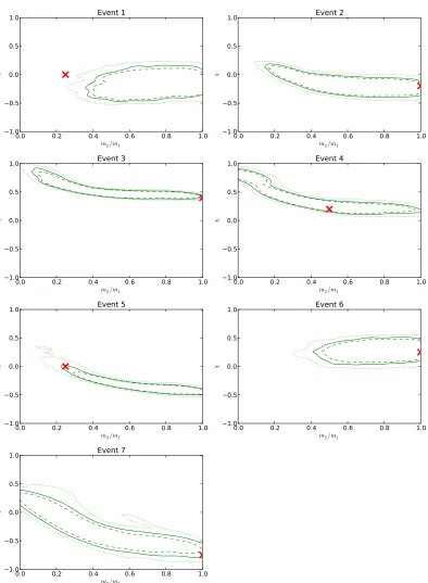
Parameter estimation algorithms have come a long way since the first NINJA project. Previously these analyses were unable to estimate the parameters of high mass systems accurately due to the use of inspiral-only models on data with little measurable inspiral. We show that these tools are now capable of reliably providing parameter estimates for both low and high mass systems. For all but one injection the masses and spins of the black holes were recovered within the estimated 95% credible regions. The remaining injection suffered small systematic biases due to non-Gaussian features present in the noise, the modeling of which is an ongoing endeavor. We find that strong intrinsic degeneracies between the masses and black hole spins [47,48] make it difficult to constrain the masses well, for 3 of the signals the presence of a neutron star cannot be ruled out. We also investigate the ability to constrain the sky localization of the various signals and demonstrate how even low power non-Gaussian noise transients in the data can effect the recovery of the intrinsic parameters of BBH systems.
We use large sets of known waveforms to assess the efficiency of the matched-filter BBH search algorithm as a function of the mass and angular momenta of the component black holes. These are the first such studies that have been done using real data recolored to second-generation noise curves, which include the non-Gaussian features that will be present in the data taken with Advanced LIGO and Advanced Virgo. As these results were obtained using the search pipelines and techniques that were deployed in the final observing runs of Initial LIGO and Initial Virgo, they can therefore provide a benchmark against which improvements to the search techniques can be compared and assessed.
assess the efficiency of the matched-filter BBH search algorithm to recover waveforms generated by different groups with the same parameters. We find that the efficiency of the matched-filter BBH search algorithm to recover different waveforms, generated by different groups, but with identical physical parameters, is indistinguishable up to statistical errors.
In this work we have not scaled observed masses and distances to account for cosmological effects, which will be important especially for high-mass binary black hole collisions. Therefore any masses and distances quoted should be interpreted asobserved
masses and luminosity distances.
The paper is organized as follows: In section2 we briefly summarize the waveform catalogue described more fully in [42]. Section 3 describes the LIGO/Virgo data used and the processing that was done to make it resemble anticipated advanced-detector noise. Section 4 describes how the parameters for the signals were chosen and reports the values that were selected. Section5describes the detection algorithms that were run on the data set and section 6 reports their results. Section 7 describes the parameter estimation results. Section 8 describes the results of a high-statistics analysis aimed at quantifying the sensitivity of the detection searches to the different hybrid waveforms. We conclude in section9with a discussion of how well the various algorithms performed, and implications for the Advanced detector era.
2. PN-NR Hybrid Waveforms
The NINJA-2 waveform catalog contains 60 PN-NR hybrid waveforms that were contributed by eight numerical relativity groups. This catalog and the procedures used to validate it are described in detail in [42]. We briefly summarize the NINJA-2 catalog here.
Each waveform in the NINJA-2 waveform catalog consists of a PN portion modelling the early inspiral, stitched to a numerical portion modelling the late inspiral, merger and ringdown. This ensures accurate modelling of the late portions of the waveform while simultaneously ensuring that waveforms are long enough to be scaled to masses as low as 10M without starting abruptly within the sensitive frequency band of the detectors.
Figure 1. Mass ratio qand dimensionless spinsχi of the NINJA-2 hybrid waveform submissions. Reproduced from [42].
The parameter space for aligned-spin BBH systems is four dimensional; the masses and spin magnitudes of each of the two holes. However, in the absence of matter Einstein’s equations possess a mass invariance, and a solution obtained by numerical relativity or other method may be trivially rescaled to any total mass. We therefore eliminate total mass from the parameter space of submissions leaving the ratio of the two masses, denotedq, and the dimensionless spins denotedχ1,2 which must lie between
−1< χ1,2 <1.
Tables 1and 2give a summary of the submissions for systems where the masses of the two black holes are equal and unequal, respectively. The first column of Tables 1
and 2gives a label for each waveform, to ease referring to them in later sections. These labels of the form “G2+20+20 T4” are constructed as follows: The first letter represents
the group submitting the numerical simulation:
F: The numerical relativity group at Florida Atlantic University, also using the BAM code [54, 55, 56,57].
G: The Georgia Tech group using MayaKranc [58, 59,60, 61, 62,63, 64]
J: The BAM (Jena) code, as used by the Cardiff-Jena-Palma-Vienna collaboration [65, 66,33, 67, 55,68]
L: The Lean Code, developed by Ulrich Sperhake [69, 70].
Ll: The Llama code, used by the AEI group and the Palma-Caltech groups [71,72,73]
R: The group from Rochester Institute of Technology, using the LazEv code [27, 74,
75,76].
S: The SXS collaboration using the SpEC code [77,78, 79, 80, 81,82,83,84, 85, 86].
U: The group from The University of Illinois [87].
Immediately after this letter follows the mass-ratioq=m1/m2, where the black holes are labeled such that q ≥ 1. Subsequently are the components of the initial dimensionless spin along the orbital angular momentum, multiplied by 100 (e.g. ‘+20’ corresponds to
ˆ
L·S~1/m21 = 0.2) of the more massive and the less massive black hole. The label closes with the Taylor-approximant being used for the PN portion of the waveform, with “T1” and “T4” representing TaylorT1 and TaylorT4, respectively. The Georgia Tech group submitted four pairs of simulations where each pair simulates systems with identical physical parameters, stitched to the same PN approximant. These waveforms are not identical however as each simulation within a pair has a different number of NR cycles and was generated at a different resolution. These are distinguished by appending “ 1” and “ 2” to the label.
by hybridization or integration from the Newman-Penrose curvature scalarψ4 to strain. Where multiple simulations were available for the same physical parameters these simulations were compared using the matched-filteroverlap. The inner product between two real waveforms s1(t) and s2(t) is defined as
(s1 s2) = 4<
Z ∞
0
df s˜1(f)˜s
?
2(f)
Sn(f)
(1)
where ˜xdenotes the Fourier transform ofxandSn(f) is the power spectral density, which
was taken to be the target sensitivity for the first advanced-detector runs, referred to as the “early aLIGO” PSD. This is described in more detail in section 3.
The overlap is then obtained by normalization and maximization over relative time and phase shifts, ∆t and ∆φ.
hs1 s2i:= max ∆t,∆φ
(s1 s2)
p
(s1 s1) (s2 s2)
. (2)
The investigations in [42] demonstrated that the submitted waveforms met the requirements as outlined above and in addition were consistent with each other to the extent expected. We therefore conclude that these submissions model real gravitational waves with sufficient accuracy to quantitatively determine how data-analysis pipelines will respond to signals in next-generation gravitational-wave observatories.
The NINJA-2 waveforms cover the 3-dimensional aligned-spin parameter space rather unevenly, as indicated in figure1. The configurations available fall predominantly into two 1-dimensional subspaces: (i) Binaries of varying mass-ratio, but with non-spinning black holes. (ii) Binaries of black holes with equal-mass and equal-spin, and with varying spin-magnitude. Future studies, with additional waveforms covering the gaps that are clearly evident in figure 1and waveforms including precession [88,89,43], would be useful to more fully understand the response of search codes across the parameter space, and would help to better tune analytical waveform models including inspiral, merger and ringdown phases.
3. Modified Detector Noise
In this section we describe the techniques used in this work to emulate data that will be taken by second generation gravitational wave observatories. This was accomplished by recoloring data taken from the initial LIGO and Virgo instruments to predicted 2015 – 2016 sensitivities. Recoloring initial LIGO and Virgo data allows the non-Gaussianity and non-stationarity of that data to be maintained.
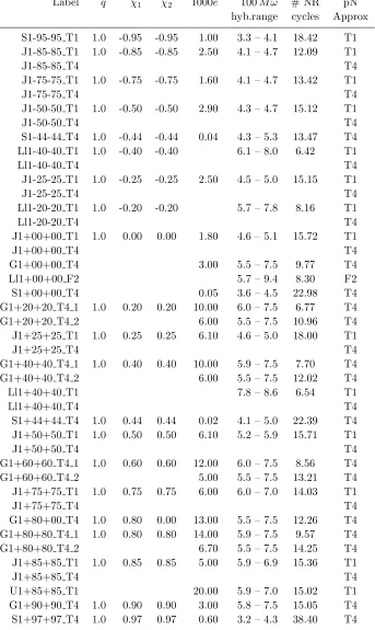
Table 1. Summary of the contributions to the NINJA-2 waveform catalog withm1=
m2. Given are an identifying label, described in section2, mass-ratioq=m1/m2which
is always 1 for these simulations, magnitude of the dimensionless spinsχi = Si/m2i, orbital eccentricitye, frequency range of hybridization inM ω, the number of numerical cycles from the middle of the hybridization region through the peak amplitude, and the post-Newtonian Taylor-approximant(s) used for hybridization.
Label q χ1 χ2 1000e 100M ω # NR pN
hyb.range cycles Approx
S1-95-95 T1 1.0 -0.95 -0.95 1.00 3.3 – 4.1 18.42 T1
J1-85-85 T1 1.0 -0.85 -0.85 2.50 4.1 – 4.7 12.09 T1
J1-85-85 T4 T4
J1-75-75 T1 1.0 -0.75 -0.75 1.60 4.1 – 4.7 13.42 T1
J1-75-75 T4 T4
J1-50-50 T1 1.0 -0.50 -0.50 2.90 4.3 – 4.7 15.12 T1
J1-50-50 T4 T4
S1-44-44 T4 1.0 -0.44 -0.44 0.04 4.3 – 5.3 13.47 T4
Ll1-40-40 T1 1.0 -0.40 -0.40 6.1 – 8.0 6.42 T1
Ll1-40-40 T4 T4
J1-25-25 T1 1.0 -0.25 -0.25 2.50 4.5 – 5.0 15.15 T1
J1-25-25 T4 T4
Ll1-20-20 T1 1.0 -0.20 -0.20 5.7 – 7.8 8.16 T1
Ll1-20-20 T4 T4
J1+00+00 T1 1.0 0.00 0.00 1.80 4.6 – 5.1 15.72 T1
J1+00+00 T4 T4
G1+00+00 T4 3.00 5.5 – 7.5 9.77 T4
Ll1+00+00 F2 5.7 – 9.4 8.30 F2
S1+00+00 T4 0.05 3.6 – 4.5 22.98 T4
G1+20+20 T4 1 1.0 0.20 0.20 10.00 6.0 – 7.5 6.77 T4
G1+20+20 T4 2 6.00 5.5 – 7.5 10.96 T4
J1+25+25 T1 1.0 0.25 0.25 6.10 4.6 – 5.0 18.00 T1
J1+25+25 T4 T4
G1+40+40 T4 1 1.0 0.40 0.40 10.00 5.9 – 7.5 7.70 T4
G1+40+40 T4 2 6.00 5.5 – 7.5 12.02 T4
Ll1+40+40 T1 7.8 – 8.6 6.54 T1
Ll1+40+40 T4 T4
S1+44+44 T4 1.0 0.44 0.44 0.02 4.1 – 5.0 22.39 T4
J1+50+50 T1 1.0 0.50 0.50 6.10 5.2 – 5.9 15.71 T1
J1+50+50 T4 T4
G1+60+60 T4 1 1.0 0.60 0.60 12.00 6.0 – 7.5 8.56 T4
G1+60+60 T4 2 5.00 5.5 – 7.5 13.21 T4
J1+75+75 T1 1.0 0.75 0.75 6.00 6.0 – 7.0 14.03 T1
J1+75+75 T4 T4
G1+80+00 T4 1.0 0.80 0.00 13.00 5.5 – 7.5 12.26 T4
G1+80+80 T4 1 1.0 0.80 0.80 14.00 5.9 – 7.5 9.57 T4
G1+80+80 T4 2 6.70 5.5 – 7.5 14.25 T4
J1+85+85 T1 1.0 0.85 0.85 5.00 5.9 – 6.9 15.36 T1
J1+85+85 T4 T4
U1+85+85 T1 20.00 5.9 – 7.0 15.02 T1
G1+90+90 T4 1.0 0.90 0.90 3.00 5.8 – 7.5 15.05 T4
Table 2. Summary of the contributions to the NINJA-2 waveform catalog with
m1> m2. Given are an identifying label, described in section2, mass-ratioq=m1/m2
magnitude of the dimensionless spins χi = Si/m2i, orbital eccentricity e, frequency range of hybridization in M ω, the number of numerical cycles from the middle of the hybridization region through the peak amplitude, and the post-Newtonian Taylor-approximant(s) used for hybridization.
Label q χ1 χ2 1000e 100M ω # NR pN
hyb.range cycles Approx
J2+00+00 T1 2.0 0.00 0.00 2.30 6.3 – 7.8 8.31 T1
J2+00+00 T4 T4
G2+00+00 T4 2.50 5.5 – 7.5 10.42 T4
Ll2+00+00 F2 6.3 – 9.4 7.47 F2
S2+00+00 T2 0.03 3.8 – 4.7 22.34 T2
G2+20+20 T4 2.0 0.20 0.20 10.00 5.6 – 7.5 11.50 T4
J2+25+00 T1 2.0 0.25 0.00 2.00 5.0 – 5.6 15.93 T1
J2+25+00 T4 T4
J3+00+00 T1 3.0 0.00 0.00 1.60 6.0 – 7.1 10.61 T1
J3+00+00 T4 T4
S3+00+00 T2 0.02 4.1 – 5.2 21.80 T2
F3+60+40 T4 3.0 0.60 0.40 1.00 5.0 – 5.6 18.89 T4
J4+00+00 T1 4.0 0.00 0.00 2.60 5.9 – 6.8 12.38 T1
J4+00+00 T4 T4
L4+00+00 T1 5.00 5.1 – 5.5 17.33 T1
S4+00+00 T2 0.03 4.4 – 5.5 21.67 T2
S6+00+00 T1 6.0 0.00 0.00 0.04 4.1 – 4.6 33.77 T1
R10+00+00 T4 10.0 0.00 0.00 0.40 7.3 – 7.4 14.44 T4
101 102 103
Frequency [Hz]
10−24 10−23 10−22 10−21
√ PSD
[1
/
√ Hz]
Early Adv. Virgo Rescaled Early Adv. Virgo Adv. Virgo design Early aLIGO aLIGO ZDHP
0 50 100 150 200
Total mass (M)
102 103 104
Horizon
distance
(Mp
c)
[image:20.612.126.488.181.609.2]early aLIGO Rescaled early AdV
Figure 2. Left: predicted sensitivity curves for aLIGO and AdV. Shown are both the design curves and predicted 2015 – 2016 early sensitivity curves. Also shown is the early AdV noise curve rescaled such that the horizon distance for a (10M,
10 M) binary system is equal to that obtained with the early aLIGO noise curve.
sensitivity curves. It is clear from the figure that the predicted sensitivity of early AdV is significantly greater than that of the early aLIGO curve, when using the predictions given in [90]. In the right panel of figure 2 we show the distance at which optimally oriented, optimally located, non-spinning, equal mass binaries would be detected with a signal-to-noise ratio (SNR) of 8 using both noise curves. This is commonly referred to as the horizon distance. The early AdV noise curve was rescaled by a factor of 1.61 so that the sensitive distance for a (10 M, 10 M) binary merger would be equal to
the early aLIGO noise curve. This rescaling was found to better reflect the updated predicted sensitivities presented in [2]. The results in this paper are generated using the early aLIGO and rescaled early AdV sensitivity curves.
As with the initial science runs, we expect data taken from these detectors, in the absence of gravitational-wave signals, to be neither Gaussian nor stationary. It is important that search pipelines demonstrate an ability to deal with these features. To simulate data with advanced detector sensitivities and with realistic non-Gaussian and non-stationary features, we chose to use data recorded by initial LIGO and Virgo and recolor that data to the predicted early sensitivity curves of aLIGO and AdV. The data we chose to recolor was data taken during LIGO’s sixth science run and Virgo’s second science run.
The procedure for producing suchrecolored data was accomplished in the following steps, which were conducted separately for the two LIGO detectors and Virgo.
• Identify a two-month duration of initial detector data to be recolored
• Measure the power spectral density (PSD) for each distinct section of science mode data using the PSD estimation routines in the lal software package [91].
• Calculate an average PSD over the two month period by taking, for every discrete value of frequency recorded in the PSDs, the median value over each of the PSDs in the set.
• Remove any line features from the resulting PSD and from the predicted early noise curves. This is done because it is difficult to remove or introduce line features from the data without introducing unwanted artifacts. Therefore it is simpler to remove line features in the PSDs, which will have the effect of preserving the line features of the original data into the recolored data.
• For each frequency bin, record the median value of the PSD over each section of science mode
• Take the ratio of the median PSD and the predicted early advanced detector noise curve. This is the reweighting to be used when recoloring.
• Using the time domain filtering abilities of thegstlalsoftware package [92], recolor the data using this reweighting factor.
Figure 3. Sensitivity curves of the recolored data for the LIGO Hanford detector (left) and the Virgo detector (right). In both cases the black dashed line shows the predicted 2015 – 2016 sensitivity curve (with the scaling factor added for Virgo). The dark colored region indicates the range between the 10 % and 90 % quantiles of the PSD over time. The lighter region shows the range between the minimum and maximum of the PSD over time.
0 5 10 15 20
Time (s)
0 200 400 600 800 1000 1200 1400 1600 1800
Signal
to
noise
ratio
0 5 10 15 20
Time (s)
0 200 400 600 800 1000 1200 1400 1600 1800
Signal
to
noise
ratio
Figure 4. SNR time series in a 20 s window around a known glitch in the original data (left) and in the recolored data (right). While the SNR time series clearly change, the primary features of the glitch are preserved across the recoloring procedure. These SNR time series were obtained by matched-filtering a short stretch of recolored and original data against a (23.7,1.3)M template.
average, we show the 10 % and 90 % quantiles as well as the maximum and minimum values for the PSD of the recolored data. We notice that the sensitivity of the detector still varies with time, as in the initial data, and that the lines in the initial spectra are still present.
[image:22.612.81.503.365.519.2]SNR time series are very comparable. As in searches on the original data, we attempt to mitigate the effect of such features. A set of data quality flags were created for the initial detector data [93,94]. These attempt to flag times where a known instrumental or environmental factor, which is known to produce non-Gaussian artifacts in the resulting strain data, was present. To simulate these data quality flags in our recolored data we simply used the same flags that were present in the original data and apply them to the recolored data.
4. Injection Parameters
As an unbiased test of the process through which candidate events are identified for BBH waveforms, 7 BBH waveforms were added to the recolored data. The analysts were aware that “blind injections” had been added, however the number and parameters of these simulated signals were not disclosed until the analyses were completed. This was similar to blind injection tests conducted by the LIGO and Virgo collaborations in their latest science runs [46]. These injections are self-blinded to ensure that no bias from knowing the parameters of the signal, or indeed whether a candidate event is a signal or a noise artifact, affects the analysis process.
The 7 waveforms added to the data were taken from the numerical relativity simulations discussed in section 2. The parameters of the blind injections are given in Table 3. The distribution of physical parameters used in these blind injections was not intended to represent any physical distribution. Instead, the injections were chosen to test the ability to recover BBH systems across a wide range of parameter space. We describe the results of searches for these blind injections in section 6 and of parameter estimation studies on these signals in section 7.
As well as these blind injections, a large number of (non-blind) simulated signals were subsequently analyzed to obtain sufficient statistics to adequately evaluate the sensitive distances at which the NR waveforms could be detected in the early aLIGO and early AdV simulated data sets. For each of the 60 NR waveforms given in Table 1
and used in results in section 8, a set of ∼ 42000 simulated signals was generated, necessarily with the same mass ratio and spins as the provided NR waveform. The total mass was chosen from a uniform distribution between 10 and 100 M. The simulations
were distributed uniformly in distance, however they were not injected beyond a distance where they could not possibly be detected. The mass-dependent maximum distance that we chose to use is given by
Dmax =
M
1.219M
5/6
175 Mpc. (3)
Here 1.219M is the chirp mass of a (1.4 + 1.4)M binary system. The factor of M5/6
Table 3. The details of the blind injections that were added to the NINJA-2 datasets prior to analysis. In this table the Event ID will be used throughout the paper to refer to specific injections. The network SNR of each injection is denoted by ρN. This is
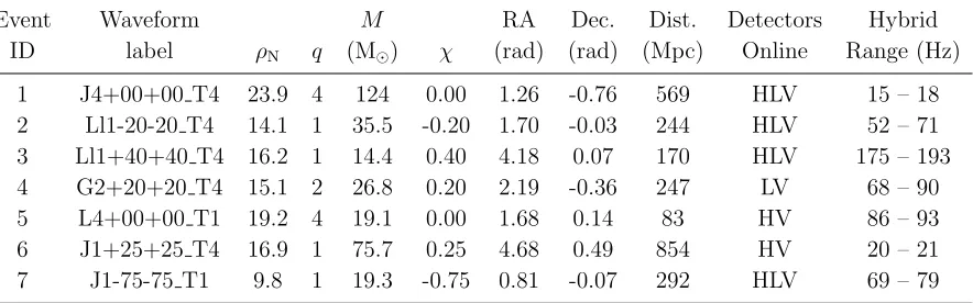
the sum of the overlaps of the injection with itself in each detector, using 30 Hz as the starting frequency in the overlap integrals. M denotes the total mass andqthe mass ratio. χ denotes the spin on each black hole, in all 7 cases both black holes in the binary had the same spin. RA and dec give the right ascension and declination of the signals respectively. Dist. denotes the distance to the source. Detectors online lists the detectors for which data is present at the time of signal. Hybridization range gives the range of frequencies in which the signal is hybridized between the post-Newtonian and numerical components. Waveform label indicates which numerical waveform was used, as shown in Tables1and2.
Event Waveform M RA Dec. Dist. Detectors Hybrid
ID label ρN q (M) χ (rad) (rad) (Mpc) Online Range (Hz)
1 J4+00+00 T4 23.9 4 124 0.00 1.26 -0.76 569 HLV 15 – 18
2 Ll1-20-20 T4 14.1 1 35.5 -0.20 1.70 -0.03 244 HLV 52 – 71
3 Ll1+40+40 T4 16.2 1 14.4 0.40 4.18 0.07 170 HLV 175 – 193
4 G2+20+20 T4 15.1 2 26.8 0.20 2.19 -0.36 247 LV 68 – 90
5 L4+00+00 T1 19.2 4 19.1 0.00 1.68 0.14 83 HV 86 – 93
6 J1+25+25 T4 16.9 1 75.7 0.25 4.68 0.49 854 HV 20 – 21
7 J1-75-75 T1 9.8 1 19.3 -0.75 0.81 -0.07 292 HLV 69 – 79
However, to include a large margin for safety ∼ 7000 of the signals were generated with chirp-weighted distances between 175 and 350 Mpc. The orbital orientations, polarization angles and sky directions are all chosen from isotropic distributions. The signal coalescence times are drawn from a uniform distribution within our analysis window. Coalescence times were limited to times where at least two observatories were operating and no data-quality flags were active. The results of analyses on the non-blind simulated signals are given in section 8.
5. Search Pipelines
The goal of this work was to evaluate the detection sensitivity to binary black hole systems, modelled from the latest numerical simulations, using the search pipelines that were used to search for gravitational-wave transient signals in data taken during the final initial LIGO and Virgo joint observing run. The two pipelines that were used to do this were the dedicated compact binary coalescence (CBC) search pipeline “ihope”
[96,97,98,46,37,44] and the unmodelled burst pipeline “Coherent WaveBurst” (cWB) [99, 100, 45, 101]. The ihope pipeline was developed as a search pipeline for detecting compact binary mergers. It employs a matched-filtering algorithm against a bank of template waveforms [44]. Theihope pipeline was used to search for CBC systems (not just binary black holes) with component masses ∈ [1,99] M. As a complement to
search pipeline, hence, it does not requirea priori knowledge of the signal waveforms. It is better suited for burst signals spanning a small time-frequency volume. Moreover, due to the lack of model constraints, cWB is more adversely affected by background noise than matched-filter searches. Past simulation studies with initial LIGO sensitivity curves have shown that cWB was sensitive to CBC mergers with total masses ∈ [25,500] M
over wide regions of the binary parameter space [102].
In addition to the ihope and cWB detection pipelines we also use parameter estimation algorithms to provide estimates of the parameters of compact binary systems observed with the detection algorithms. In the following section we provide a brief overview of the detection and parameter estimation pipelines. The results of running these searches on the data containing the NINJA-2 blind injections are presented in section 6and parameter estimation results given in section 7.
5.1. Coherent WaveBurst
Coherent WaveBurst is a multi-resolution algorithm for coherent detection and reconstruction of gravitational wave bursts [22]. The cWB algorithm has been used in various LIGO-Virgo burst searches [99, 100, 45] and more recently in the search for intermediate mass black hole binaries [101]. Within the framework of the constrained maximum likelihood analysis [22], cWB identifies GW signals in data from multiple detectors and provides estimates of the signal parameters, e.g. sky location and waveforms. Along with the reconstruction of un-modeled burst signals, which imply random polarization, cWB can perform loosely modeled likelihood analyses assuming different polarization states, i.e. elliptical, linear or circular.
The NINJA2 cWB analysis uses the elliptical polarization constraint [102,101] and searches for signals in the frequency band from 32 Hz to 1024 Hz. The analysis is performed in several steps: first, the data streams from all GW detectors are processed with the Meyer’s wavelet transformations with 6 different time-frequency resolutions of 4×1/8, 8×1/16, 16×1/32, 32×1/64, 64×1/128, 128×1/256 [Hz×s]. Then the data are conditioned with a linear predictor error filter to remove power lines, violin modes and other predictable data components. Triggers are reconstructed as the coherent sets of samples (pixels) identified in the time-frequency data. For each trigger the coherent statistics are then computed. These include the network correlation coefficient,
5.2. ihope
The ihope pipeline is designed to search for gravitational waves emitted by coalescing compact binaries [44]. It has been optimized for and used in LIGO and Virgo GW searches over the past decade [103, 96, 97, 104, 46, 37], and also in the mock Laser Interferometer Space Antenna (LISA) data challenges [105]. The NINJA-2 ihope
analysis uses the same pipeline-tuning that was used in the searches performed during the final initial LIGO and Virgo joint observing run [46].
The pipeline matched-filters the detector data against a bank of analytically modelled compact binary merger waveforms [19,44]. Only nonspinning compact binary merger signals are used as filters and the bank is created so as to densely sample the range of possible binary masses [106]. For each detector, the filtering stage produces a sequence oftriggers which are plausible events with a high signal to noise ratio SNRρ. The algorithm proposed in [107] is used to keep only those that are found coincident in more than one detector across the network, which helps remove triggers due to noise. Knowledge of the instrument and its environment is used to further exclude triggers that are likely due to non-Gaussian noise transients, or glitches. Periods of heightened glitch rate are removed (vetoed) from the analysis. The time periods where the rate of glitches is elevated are divided into 3veto categories. Periods of time flagged by category 1 and 2 vetoes are not included in the analysis as known couplings exist between instrumental problems and the gravitational-wave channel during these periods. Periods of time vetoed at category 3 are likely to have instrumental problems. A strong gravitational-wave signal can still be detected during category 3 times, but including these periods in the background estimate can compromise our ability to detect weaker signals in less glitchy periods of time. For this reason the search is performed both before and after category 3 vetoes are applied. The significance of events that survived category 1-3 vetoes were calculated using the background that also survived categories 1-3. The significance of events that survived category 2 but were vetoed at category 3 were calculated using background that survived categories 1-2.
Signal based consistency measures further help distinguish real signals from background noise triggers in those that are not vetoed and pass the coincidence test. Theχ2 statistic proposed in [108] quantifies the disagreement in the frequency evolution of the trigger and the waveform template that accumulated the highest SNR for it, c.f. Eq. (4.14) of [108]. We weight the SNR with this statistic to obtain thereweighted SNRs for all coincident triggers. The exact weighting depends on the mass range the search is focused on, c.f. Eq. (17,18) of [44]. The reweighted SNR is used as the ranking statistic to evaluate the significance, and thus the false alarm rate (FAR), of all triggers.
Following the division of the mass-parameter space used in [46,37], we performed both low mass and high mass ihope searches on the NINJA-2 data. The low-mass search focused on binaries with 2M ≤m1+m2 <25M, and used frequency domain
inspiral-merger-ringdown model calibrated to numerical relativity, as described in [29]. The exact
χ2-weighting used to define the re-weighted SNR varied between the two analyses [44]. The significance of the triggers found by both was estimated as follows. All coincident triggers are divided into 4 categories, i.e. HL, LV, HV and HLV, based on the detector combination they are found to be coincident in [46]. They are further divided into 3
mass-categories based on their chirp mass Mc = (m1m2)3/5(m1 +m2)−1/5 for the low-mass search, and 2 categories based on their length in time for the high-low-mass search [46]. The rate of background noise triggers, orfalse alarms, has been found to be significantly higher for shorter signals from more massive binaries, and also to be different depending on the detector combination, and these categorizations help segregate these effects for estimation of the background [46,44]. For all the triggers the combined re-weighted SNR
ˆ
ρ is computed, which is the quadrature sum of re-weighted SNRs across the network of detectors. All triggers are then ranked in each of the mass and duration sub-categories independently according to their ˆρ, allowing us to put a limit on the trigger false alarm rate (FAR) at a given threshold ˆρ= ˆρ0. This is described by
FAR (ˆρ0)≤ N(ˆρ≥ρˆ0) + 1
Tc
, (4)
where N(ˆρ ≥ x) is the number of background noise triggers with ˆρ greater than or equal to x, and Tc is the total time analyzed for that coincidence category. From 4, the smallest FAR we can estimate is 1/Tc, and to get a more precise estimate
for our detection candidates we simulate additional background time. We shift the time-stamps on the time-series of single detector triggers by ∆t relative to the other detector(s), and treat the shifted time-series as independent coincident background time. All coincident triggers found in the shifted times would be purely due to background noise. We repeat this process setting ∆t=±5s,±10s,±15s, . . ., recording all the time-shifted coincidences, until ∆t is larger than the duration of the dataset itself. With the additional coincident background time Tc accumulated in this way, we can get a
more precise estimate of the low FARs we expect for detection candidates, which are described in detail in section 6.2.
5.3. Parameter estimation
The detection methods described above produce times of interest where a gravitational wave may be present in the data (i.e. triggers), along with point estimates of the compact object masses from the signal, independently in each detector. These triggers are followed up with the goal of estimating the posterior probability density function of the parameters that describe the signal and to evaluate the evidence of different waveform models. In order to do so, we use Bayesian methods, in which the data from all detectors are analysed coherently.
![Figure 1.Mass ratiosubmissions. Reproduced from [ q and dimensionless spins χi of the NINJA-2 hybrid waveform42].](https://thumb-us.123doks.com/thumbv2/123dok_us/1622651.115372/16.612.83.508.81.424/figure-mass-ratiosubmissions-reproduced-dimensionless-ninja-hybrid-waveform.webp)
![Figure 2.] waveform approximant.Results in this paper are generated from the early aLIGO noise curve and the rescaled10Right: Horizon distance as a function of observed total mass for the early aLIGO andrescaled early AdV sensitivity curves](https://thumb-us.123doks.com/thumbv2/123dok_us/1622651.115372/20.612.126.488.181.609/waveform-approximant-results-generated-horizon-observed-andrescaled-sensitivity.webp)