City, University of London Institutional Repository
Citation: Charalambous, T. and Kalyvianaki, E. (2010). A min-max framework for CPU
resource provisioning in virtualized servers using ∞ Filters. Decision and Control (CDC),
ℋ
2010 49th IEEE Conference on, pp. 3778-3783. doi: 10.1109/CDC.2010.5717375
This is the accepted version of the paper.
This version of the publication may differ from the final published
version.
Permanent repository link: http://openaccess.city.ac.uk/8178/
Link to published version: http://dx.doi.org/10.1109/CDC.2010.5717375
Copyright and reuse: City Research Online aims to make research
outputs of City, University of London available to a wider audience.
Copyright and Moral Rights remain with the author(s) and/or copyright
holders. URLs from City Research Online may be freely distributed and
linked to.
A Min-Max Framework for CPU Resource Provisioning
in Virtualized Servers using
H
∞Filters
Themistoklis Charalambous and Evangelia Kalyvianaki
Abstract— Dynamic resource provisioning for virtualized server applications is integral to achieve efficient cloud and green computing. In server applications unpredicted workload changes occur frequently. Resource adaptation of the virtual hosts should dynamically scale to the updated demands (cloud computing) as well as co-locate applications to save on energy consumption (green computing). Most importantly, resource transitions during workload surges should occur while mini-mizing the expected loss due to mismatches of the resource predictions and actual workload demands. Our approach is to minimize the maximum expected loss using the same techniques as in two-person zero-sum games. We develop an H∞ filter that minimizes the worst-case estimation and allocate resources fast. Through simulations our H∞ filter demonstrates its effectiveness and good performance when compared against Kalman-based controllers.
I. INTRODUCTION
Virtualization of data centers has given rise to important paradigms namely cloud and green computing. Cloud com-puting provides an execution platform of essential means (i.e. computing resources and software components) that applications can use on demand. Applications might include for example web and database servers which can be hosted within one machine or span across machines. In addition, green computing utilizes machines power in ways to reduce their energy consumption as well as power and cooling expenses.
Modern virtualization (e.g. [1]) is one of the key contribut-ing factors to both paradigms. When virtualized, a machine is transformed into one or more virtual execution environments,
called virtual machines (VMs) where applications can run
in isolation and share the machine resources by runtime resource allocation. In cloud computing, virtualization is used to dynamically create VMs according to the application demands and online adjust their resource allocations to match their workload needs. Furthermore, virtualization is also used to reduce the required machines to host a certain number of server applications. This is achieved by application consoli-dation to a smaller group of hosting machines where unused machines are switched off for reduced energy consumption. To achieve efficient virtualization it is essential to ensure performance guarantees for each co-located application and provide them with resources according to their demands and meet their Service Level Objectives (SLOs). However, ap-plications exhibit highly changing workload demands which cause difficult to predict resource fluctuations [2], [3]. There
Themistoklis Charalambous is at the Electrical and Computer Engi-neering Department, University of Cyprus, Cyprus and Evagelia Kaly-vianaki is at the Department of Computing, Imperial College London, UK
[email protected], [email protected]
is the need forautonomic resource managementmethods that
adaptively allocate resources across virtualized applications with diverse workload and internal structure characteristics. Autonomic resource management in a virtualized environ-ment using control-based techniques has recently gained sig-nificant attention. The most widely-used approach to control the application performance is by controlling its CPU utiliza-tion within the VM, for example [4], [5]. This approach is further extended to dynamically distribute resources among co-located applications under conditions of contention [4], [6]. Finally, special attention has been given to model the resource coupling in multi-tier virtualized applications to provide timely allocations during workload changes [5], [7]. A key performance metric for these controllers is their re-sponsiveness to sudden workload changes. Their parameters can be tuned to achieve transition phases of smaller duration, however, they do not provide any sort of control over the maximum error of the application performance.
The maximum error occurs under conditions of contention. In a virtualized application—resources are constantly up-dated to match the workload demands while freeing up resources for other applications—it is anticipated that the ap-plication exhibits short but very frequent periods of resource contention. It is thus important to optimize performance to recover after these periods. To the best of our knowledge, this is the first approach to control the maximum error of the performance of a virtualized application in conditions of contention.
This paper treats the problem as a game against nature and minimizes the maximum expected loss using the same techniques as in the two-person zero-sum games [8]. It
presents a new discrete-time controller based on the H∞
filter, which minimizes the worst-case estimation error
(min-max). The H∞ controller allocates CPU resources in
vir-tualized applications and minimizes the maximum error in their performance as measured by the requests mean response
time (mRT). Simulation results show that the H∞ controller
lowers mRT during saturation when compared against a Kalman controller.
In Section II we provide further motivation and discuss related work. In Section III we provide the notation used throughout this paper. Section IV describes the models
adopted for the resource utilization and the mRT. In
Sec-tion V, the H∞ filter is designed, while in Section VI,
the performance of the H∞ filter is evaluated. Finally, we
II. BACKGROUND
A. Motivation
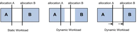
Adequate provisioning for VMs’ resources is crucial for a high performance data center. Consider a server con-solidation example with two single-component applications hosted on a single physical server machine. Assume that each application has known workload requirements and the sum of resources from both applications does not exceed the total available physical resources for the server machine. The left diagram in Figure 1 illustrates two VMs, each one hosting an application with resources allocated as required. In this way, both applications are served adequately and the total resource utilization of the physical machine is now increased simply by co-locating two running servers.
Consider now the case where the workload in both ap-plications changes, (middle diagram in Figure 1). In VM A it increases, therefore more resources are required, while in VM B it decreases so fewer resources are needed. In the case of VM A, the under-provisioning results in performance degradation, since the application does not have enough resources to serve its incoming requests. In the case of VM B, the over-provisioning does not affect the running application within the VM B. However it does reduce the free available resources for a third VM to be placed on the same machine. Therefore, in both cases, the resource allocation needs to adapt to the new resource demands (right most diagram in Figure 1).
This paper concentrates on the dynamic case of the resource adaptation while workload demands change. Our work makes use of modern virtualization platforms which export a user-level interface to bound the maximum resource allocation per VM at runtime.
B. Related Work
Autonomic resource management aims to adjust resource allocations across applications to meet their SLOs as mea-sured by the application response times. In [9] and [10], the authors directly control application response times through runtime resource CPU allocation using an offline system identification analysis to model the relationship between the response times and the CPU allocations in regions where it is measured to be linear. However, as this relationship is application-specific and relies on offline identification performance models, other approaches, such as [11] and [10], control the response times in combination with the applica-tion CPU utilizaapplica-tion.
The application performance can be controlled, by control-ling is CPU utilization. As long as the utilization remains below the allocation by a certain threshold the application response times stay low [12]. Furthermore, when the utiliza-tion approaches the allocautiliza-tion, the response times increase dramatically and the application performance drops. Padala
et al.[4] present a two-layer non-linear controller to regulate the utilization of the virtualized components of multi-tier applications. Kalyvianaki et al.[5] formulate the regulation problem as a CPU utilization tracking one and present
Fig. 1. Resource management example in virtualized applications. Shaded rectangles show resource utilizations and solid lines indicate allocated resources.
adaptive Kalman-based controllers to track and maintain the CPU utilization to a user-defined threshold. However, the Kalman filter provides an optimal estimate if the model and the noise statistics are known. Otherwise, it may perform poorly if there are errors in the system model or the assumed noise statistics.
In addition, [4], [6] control the resource allocations across consolidated virtualized applications under conditions of contention. When applications demand more resources than physically available the above controllers distribute resources among them in ways to respect their user-given priorities. Finally, in [7] and [5] Multi-Input-Multi-Output (MIMO) feedback controllers are presented. These controllers make global decisions by coupling the resource usage of all components of multi-tier server applications.
A key performance metric for controllers used for vir-tualized servers is their responsiveness to sudden workload changes. [5], [6] study the performance of their controllers across their parameters against significant resource fluctua-tions until the controllers stabilize to the new demands. The parameters of the controllers in [5] can be tuned to achieve transition phases of smaller duration, however, they do not provide any sort of control over the maximum error of the application performance. TheH∞ controller presented here
is designed to minimize the max error caused by saturation periods.
III. NOTATION
Vectors are denoted by small, bold letters whereas matrices are denoted by capital letters. AT and A−1 denote the
transpose and inverse of matrix A respectively. For two
symmetric matrices A and B, A � B means that A−B
is positive definite andA �B means that A−B is
semi-positive definite. By I we denote the identity matrix. aˆk
denotes the estimate of random vectorak for time instantk. Pk denotes the matrix P at time instant k. The norm of a vector or a matrix is given by � · �. a ∈ RN+×1 represents
a vector with N nonnegative real entries and A ∈ RN+×N
represents a nonnegative matrix, i.e. all entries in the matrix are nonnegative.
IV. SYSTEMMODEL
A. mRT model
[image:3.612.324.547.65.120.2]!"#$"#
%&'( )&
*&
Fig. 2. Model of the demandDin a server.
requests. For instance, in the case of a single server M/M/1, this is given by: mRT =s/(1−u)(Little’s law), where s
is the mean service time and u the mean utilization. This
model predicts that when the utilization reaches saturation the mRT goes to infinity. This is the case where the server has no more resources to serve new requests, and hence these are kept in the input queues and their waiting times grow indefinitely. However, in a virtualized environment when the server is saturated, we can dynamically increase its resource allocations and therefore provide more resources to serve new incoming requests and those already waiting in the queue. In this way, as long as the server is saturated the requests mRT will grow, however, it will drop when the server exits saturation and has enough resources to server all requests. This section provides a function of themRTwhich models the above characteristics. We do not aim to provide an accuratemRTprediction model, rather, we use this model as the cost function to evaluate the performance of theH∞ controller in a simulated environment. This model is solely based on well known characteristics of server applications described below.
It is very difficult to predict the exact values of the
mRT of server applications across operating regions and different applications and workloads. However, it is known to have certain characteristics [12]. Generally, its values can be divided into three regions: (a) when the application is provisioned with abundant resources all requests are served as they arrive and the response times are kept low; (b) when the utilization approaches 100% (e.g. around 70-80% on average) the mRT increases above the low values from the previous region because there are instances at which the requests peak and approach 90-100%; (c) however, when resources are scarce and very close to 100%, requests compete for limited resources, they wait in the input queues and their response times increase dramatically to relatively high values.
It is often the case, for instance in data centers that to maintain good server performance the operators aim to keep machine CPU utilization below 100% of the machine capacity by a certain value, which is usually called head-room. Headroom values denote the boundary between the second and the thirdmRTregions. At these values the server is well provisioned and response times are kept low. If the utilization approaches 100% due to increased workload demands, operators increase the server resources.
In order to assimilate these characteristics into the system we propose the followingmRTmodel defined in (1), where themRTis given as a function of the ratio between workload
0 0.2 0.4 0.6 0.8 1
0 0.5 1 1.5 2 2.5 3
CPU Demand/CPU allocation
[image:4.612.365.510.53.171.2]mRT (s)
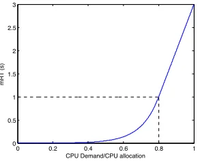
Fig. 3. mRTmodel with respect to CPU usage, whereγ= 10andφ= 0.8.
demandD and allocationa:
mRT(D/a) =
�
eγ(D
a−φ), if D
a ≤1
1 +γ(D
a −φ), if D
a >1
(1)
First, we define the demandD, in terms of CPU, at time
instantk. This is given by:Dk+1=Dk−uk+ik+1, whereuk is the CPU utilization at time instantkandik+1 is the CPU from the requests at time instantk+1. A graphical illustration of the demand model in a server is given in Figure 2. We then include the headroom valueφand we also use the constant γto assign some large response time values in regions close to saturation.
Figure 3 graphically illustrates the response time model when γ = 10 and φ = 0.8. It is easy to distinguish the three regions aforementioned: (a) When D/a < 0.7, the mRT is much lower than 1 second (s). For the rest of this paper we will use the 1s threshold to denote a timely completed request; (b) when 0.7 ≤ D/a ≤ 0.8, then the mRT increases, but since there are still resources it remains below the threshold; (c) when D/a > 0.8 we assume that some requests remain in the input queue due to the fluctuations in demand and hence, the mRT is varying linearly with the demand. Note that D/a > 1 means that the maximum amount of resources has been allocated and queues are growing in the input, making the demand even bigger, thus increasing themRT.
For the rest of this paper, we will use (1) along with the Root-Mean-Square-Error (RMSE) of the allocation to evaluate the performance of the virtualized application when its CPU allocation is controlled by our H∞ filter and the other filters we use for comparison. Without loss of generality this enables us to evaluate the performance of the
H∞ filter across operating regions.
B. The CPU Usage and Allocation
The purpose of the H∞ controller is to control the allocation of the VMs running a server application while observing its utilization across VMs. We assume multi-tier server applications composed of N components, where each component runs on a different VM. We start by modeling the time-varying CPU utilization per component as a random walk given by the following linear stochastic difference equation:
wherexk ∈RN+×1is the vector of the percentages of the total CPU capacity actually used by the application components
during interval k; each row corresponds to a component.
The independent random vector rk ∈ RN+×1 represents the
process noise. The process noise models the utilization be-tween successive intervals caused by workload changes, e.g. requests being added, doing work from previous intervals, or leaving the server.
We denoteak ∈RN+×1as the CPU capacity of a physical
machine allocated to the VMs; each row corresponds to a
component. ak shows the maximum amount of resources
a VM can use. We denote uk ∈ RN+×1 as the total CPU
utilization actually observed in the VMs; again each row
corresponds to an application tier. uk models the observed
application utilization xk in addition to any usage noise
coming from other sources, such as the operating system, to support the application.
The purpose of the H∞ controller is to maintain good
server performance in the presence of workload changes. This is achieved by adjusting the allocation to values above
the utilization. For each time-intervalkthe desired
relation-ship between the two quantities is given by:
uk=Cak+vk, (3)
where C ∈ RN×N
+ is a diagonal matrix with the target
value ci for each component i along the diagonal, and
denotes the gap between the allocation and the utilization;
vk ∈ RN+×1 denotes the utilization measurement noise at
each component. To maintain good server performance, the allocation should follow the utilization and therefore is also modeled as a random walk. The allocation for the next
time-interval (k+ 1)is given by:
ak+1=ak+wk, (4)
wherewk ∈RN+×1 denotes the process noise of the
alloca-tion signal.
V. THEH∞CONTROLLER
We formulate the allocation problem as a state estimation problem. Kalman filters [13] are commonly used to estimate the states of a dynamic system and they have also been used for the allocation problem [5]. Their attractiveness relies on the fact that the Kalman filter is the optimal linear filter when minimizing at each time step the two-norm of the expected values of the estimation error. However, they do not provide any guarantees in terms of limiting the maximum estimation
error. Alternatively, H∞ filters minimize the worst-case
estimation error—they are calledminimaxfilters—and can be
used to incorporate more robustness into the state estimation problem.
The cost function for our problem formulation is given by:
J =
�N−1
k=0 �ak−ˆak�22
�a0−aˆ0�2P−1
0 +
�N−1
k=0
�
�wk�2Q−1
k
+�vk�2R−1
k
� (5)
where P0 ∈ RN×N, Q
k ∈ RN×N and Rk ∈ RN×N are symmetric, positive definite matrices defined by the problem
specifications, i.e. P0 is the initial error covariance matrix,
Qk and Rk are the process and measurement covariance
matrices for time intervalk, respectively;ˆak is the estimate
of the CPU allocation. The direct minimization ofJ in (5) is
not tractable, and as a result we choose a performance bound and our controller is designed based on that threshold. In
our problem, the target is to keep themRT below a certain
threshold (e.g. less than a second). Therefore, our controllers
are designed based on the fact that J < 1/θ, where θ is
specified such that the desiredmRTis less than a certain
user-specified threshold. Considering (5), the steady-state H∞
filter bounds the following cost function:
J = lim
N→∞
�N−1
k=0 �ak−ˆak�22
�N−1
k=0
�
�wk�2Q−1
k
+�vk�2R−1
k
�. (6)
LetGˆae be the system that hase= [w v]T as its input and
ˆ
a as its output. Since theH∞ filter makes the cost (6) less
than1/θ for allwk andvk, then according to [14]:
�Gˆae�2∞= sup ζ
�a−ˆa�2 2
�w�2
Q−1+�v�2R−1 ≤ 1
θ, (7)
where ζ is the phase of �w�2
Q−1 +�v�2R−1 comprised by
the sampling time of the system and the frequency of the
signals. Since we want themRTto be less than a certain value
(usually around1 second), we have to keep the CPU usage
to less than a threshold set by our mRT model. Therefore, using (7) we want:
sup
ζ
�Φ−C�2 2
�w�2
Q−1+�v�2R−1 ≤ 1
θ, (8)
which is equivalent to:
θ≤inf
ζ �w�2
Q−1+�v�2R−1
�Φ−C�2 2
. (9)
whereΦandCare diagonal matrices with the headroom
val-uesφiand target valuesci for each component, respectively,
along the diagonal. Inequality (9) suggests that a higher value
of θ can be accommodated when the system is very noisy
or the CPU usage uis very closed to the headroom value
φ. Note, however, that the necessary condition to ensure that
Pk remains positive definite and the system retains stability
for the aboveH∞ filter is that:
I−θPk+CTRk−1CPk �0. (10)
To design the controller we consider inequalities (9) and (10).
Note that the Kalman filter gain is smaller than the H∞
filter gain forθ >0, meaning that theH∞ filter relies more
on the measurement and less on the system model. Asθgoes
closer to zero, theH∞filter gain goes closer to the Kalman
filter gain [14].
For the cost function (5), theH∞ filter is thus given by:
Kk=Pk[I−θPk+CTRk−1CPk]−1CTR−k1 (11)
ˆ
ak+1= ˆak+Kk(uk−Cˆak) (12)
whereKk is the gain matrix andPk is the error covariance
matrix and it is positive definite (since P0 is positive def-inite and if Pk is positive definite, then from (13) positive
definiteness is preserved inPk+1).
VI. PERFORMANCEEVALUATION
In this section, we evaluate the performance of the H∞
filter using a simulated virtualized environment which we have built using MATLAB. For simplicity, a Single-Input-Single-Output (SISO) system is used, in order to high-light the characteristics of our controller. For the current evaluation we measure the performance of the controller around the mRT using (1) and the RMSE of the allocation. We compare our controller against the conceptually similar Kalman controller from [5]. Both controllers use the same utilization model, however, the Kalman controller aims to minimize the mean prediction error, while our controller minimizes the maximum error.
We evaluate the H∞ controller across two workload
conditions. First, we simulate gradual workload variations to decreasing and increasing demand. Results are shown in Section VI-A. Second, we simulate a flash crowd, where the workload demand repeatedly peaks for a very short time following a saw-tooth pattern. Results are shown in Section VI-B. In both cases, we study the performance of the
H∞ controller when the process wk and the measurement
noisevk are either normally or uniformly distributed.
Finally, the parameters used in the current evaluation are the following:c is set to 0.95 which is above the headroom valueφ= 0.8. This makes our system to constantly operate near conditions of contention, in order to better observe the
H∞ filter performance. θ is set to the high value of 0.7
because we set the system to be noisy, which is depicted by the value ofQthat we set to 4. Different values for the rest
of the parameters showed similar results and therefore they are not presented here.
A. Gradual workload changes
The performance of theH∞ controller is measured when
the utilization exhibits gradual changes towards decreasing from an initial 60% to 30% and then increasing again to 60%. We study the controller allocations when the process (wk) and measurement (vk) noises are taken to be normally
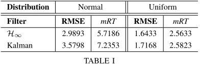
distributed in Figure 4 and when these noises are uniformly distributed in Figure 5. Numerical results for themRTand the RMSE of the allocation for the duration of the experiments are shown in Table I. The RMSE measures the error between the observed allocation and the predicted allocation, given the utilization for each interval and the headroom value c. It measures the variation of the controller’s allocations with respect to the reference valuec.
Figures 4(a) and 5(a) illustrate the allocations of the
H∞ controller as the utilization demand varies. The same
figures also show the allocations of the Kalman controller for comparison purposes. Although both controllers adjust their allocations to match the workload demands, the H∞
controller allocates resources faster during conditions of
contention than the Kalman controller. This is better shown for the intervals 50 to 80 where the workload demand increases gradually and saturation here causes the mRT to jump to high values as shown in Figures 4(b) and 5(b).
The difference between theH∞and the Kalman controller
is better shown in the case where the noises are normally distributed. In this case, the server is saturated for many intervals (i.e. intervals 50-60) and themRT increases a lot. However, as soon as the demand starts to stabilize the server is able to serve new incoming requests and those already left in its input queue. TheH∞ controller manages to serve all
requests faster than the Kalman controller as shown by the lower maximummRT. The Kalman controller also serves all requests, but itsmRTincreases to higher values. Overall, the
H∞ controller achieves better performance for the duration
of the experiment as also shown in Table I.
When the process and measurement noise are uniformly distributed the workload utilizations vary less than in the case of the normally distributed noises. When the noise is uniform, theH∞controller also recovers faster after a period
of contention; the mRT of the H∞ controller is lower than
the KalmanmRTaround the intervals50−60in Figure 5(b).
However, its overall performance for the duration of the experiment is very close to the Kalman performance, Table I. The most important aspect of the H∞ filter that
differ-entiates it from other controllers is that is minimizes the maximum error. When the noise is normal, it operates very well when compared against the Kalman controller which is designed under this assumption. In addition, the H∞
filter performs better near the maximum error for uniformly distributed noise.
B. Saw-tooth demand for CPU usage
In this case we vary the utilization in a saw-tooth structure. This is a very demanding workload, where the utilization changes rapidly from very large to very small values. In this case it is very important for the controller to adapt the allocations in a timely fashion. To achieve overall good per-formance the error during contention should be minimized.
Figures 7 and 6 illustrate the performance of the H∞
controller against the Kalman filter in cases where the process (wk) and measurement (vk) noises are taken to be
normally and uniformly distributed, respectively. Numerical results for the duration of the simulations, given in Table II, show that theH∞controller keeps themRTin both cases to
lower values than the Kalman controller. TheH∞controller
allocates resources faster during periods of contentions as also shown by its increased utilization when the workload demand increases in Figure 7(a) and 6(a).
VII. CONCLUSIONS
We have used a minimax framework and developed anH∞
0 10 20 30 40 50 60 70 80 90 100 25 30 40 50 60 70 80 90 time interval CPU (%) H!
CPU usage (H!)
Kalman CPU usage (Kalman)
(a) CPU allocations and utiliza-tions
0 10 20 30 40 50 60 70 80 90 100 0 5 10 15 20 25 30 time interval mRT (s) H! Kalman (b)mRT
Fig. 4. Gradual Workload Changes:H∞controller performance when the
process (wk) and the measurement (vk) noise arenormallydistributed.
0 10 20 30 40 50 60 70 80 90 100 25 30 40 50 60 70 80 90 time interval CPU (%) H! CPU usage (H!) Kalman CPU usage (Kalman)
(a) CPU allocations and utiliza-tions
0 10 20 30 40 50 60 70 80 90 100 1.5 2 2.5 3 3.5 4 4.5 5 time interval mRT (s) H ! Kalman (b)mRT
Fig. 5. Gradual Workload Changes:H∞controller performance when the
process (wk) and the measurement (vk) noise areuniformlydistributed.
Distribution Normal Uniform
Filter RMSE mRT RMSE mRT
H∞ 2.9893 5.7186 1.6433 2.5633
Kalman 3.5798 7.2353 1.7168 2.5823
TABLE I
RMSEANDmRTVALUES FOR GRADUAL WORKLOAD CHANGES
0 10 20 30 40 50 60 70 80 90 100 25 30 40 50 60 70 80 90 time interval CPU (%) H ! CPU usage (H!) Kalman CPU usage (Kalman)
(a) CPU allocations and utiliza-tions
0 10 20 30 40 50 60 70 80 90 100 0 5 10 15 20 25 30 35 40 time interval mRT (s) H ! Kalman (b)mRT
Fig. 6. Saw-Tooth Workload Changes:H∞controller performance when
the process (wk) and the measurement (vk) noise arenormallydistributed.
the maximum error during conditions of contention. In these
conditions, the H∞ controller provides better performance
than other approaches. But, there are no assumptions on the
noise characteristics and hence the H∞ controller is more
robust than other controllers.
REFERENCES
[1] P. Barham, B. Dragovic, K. Fraser, S. Hand, T. Harris, A. Ho, R. Neugebauer, I. Pratt, and A. Warfield, “Xen and the Art of
Virtualization,” inProceedings of the ACM Symposium on Operating
Systems Principles (SOSP), 2003, pp. 164–177.
0 10 20 30 40 50 60 70 80 90 100 25 30 40 50 60 70 80 90 time interval CPU (%) H ! CPU usage (H!) Kalman CPU usage (Kalman)
(a) CPU allocations and utiliza-tions
0 20 40 60 80 100 0 5 10 15 20 25 30 35 40 time interval mRT (s) H ! Kalman (b)mRT
Fig. 7. Saw-Tooth Workload Changes:H∞controller performance when
the process (wk) and the measurement (vk) noise areuniformlydistributed.
Distribution Normal Uniform
Filter RMSE mRT RMSE mRT
H∞ 6.0463 11.5674 4.575 10.5759
Kalman 5.7544 12.7232 5.0099 12.0326
TABLE II
RMSEANDmRTVALUES FOR SAW-TOOTH-LIKE WORKLOAD CHANGES
[2] M. Arlitt and T. Jin, “A Workload Characterization Study of the 1998
World Cup Web Site,” IEEE Network, vol. 14, no. 3, pp. 30–37,
May/June 2000.
[3] A. Iyengar, J. Challenger, D. Dias, and P. Dantzig, “High-Performance
Web Site Design Techniques,”IEEE Internet Computing, vol. 4, no. 2,
pp. 17–26, Mar/Apr 2000.
[4] P. Padala, K. Shin, X. Zhu, M. Uysal, Z. Wang, S. Singhal, A. Mer-chant, and K. Salem, “Adaptive Control of Virtualized Resources in
Utility Computing Environments,” in Proceedings of the European
Conference on Computer Systems (EuroSys), 2007, pp. 289–302. [5] E. Kalyvianaki, T. Charalambous, and S. Hand, “Self-Adaptive and
Self-Configured CPU Resource Provisioning for Virtualized Servers
using Kalman Filters,” inProceedings of the 6th International
Con-ference on Autonomic Computing (ICAC). New York, NY, USA: ACM, 2009, pp. 117–126.
[6] P. Padala, K.-Y. Hou, K. G. Shin, X. Zhu, M. Uysal, Z. Wang, S. Sing-hal, and A. Merchant, “Automated Control of Multiple Virtualized
Resources,” inProceedings of the 4th ACM European Conference on
Computer Systems (EuroSys ’09). New York, NY, USA: ACM, 2009, pp. 13–26.
[7] E. Kalyvianaki, T. Charalambous, and S. Hand, “Resource
Provi-sioning for Multi-Tier Virtualized Server Applications,” Computer
Measurement Group (CMG) Journal, vol. 126, pp. 6–17, 2010.
[8] T. Basar and P. Bernhard,H∞- Optimal Control and Related Minimax
Design Problems: A Dynamic Game Approach, 2nd ed. Boston, MA:
Birkha¨user, 1995.
[9] Z. Wang, X. Zhu, and S. Singhal, “Utilization and SLO-Based Control
for Dynamic Sizing of Resource Partitions,” inProceedings of the
IFIP/IEEE International Workshop on Distributed Systems: Opera-tions and Management (DSOM), October 2005, pp. 133–144. [10] X. Zhu, Z. Wang, and S. Singhal, “Utility-Driven Workload
Manage-ment using Nested Control Design,” inProceedings of the American
Control Conference (ACC), 2006, pp. 6033–6038.
[11] Z. Wang, X. Liu, A. Zhang, C. Stewart, X. Zhu, T. Kelly, and S. Singhal, “AutoParam: Automated Control of Application-Level
Performance in Virtualized Server Environments,” inProceedings of
the IEEE International Workshop on Feedback Control Implementation and Design in Computing Systems and Networks (FeBID), 2007.
[12] L. Kleinrock, Queueing Systems, Volume 1, Theory.
Wiley-Interscience, 1975.
[13] R. E. Kalman, “A New Approach to Linear Filtering and Prediction
Problems,”Transaction of the ASME–Journal of Basic Engineering,
vol. 82, no. Series D, pp. 35–45, 1960.
[14] D. Simon,Optimal State Estimation: Kalman, H-infinity, and
[image:7.612.66.288.53.157.2] [image:7.612.65.287.206.310.2] [image:7.612.79.275.356.419.2] [image:7.612.64.289.453.557.2]