arXiv:astro-ph/0703234v1 9 Mar 2007
Upper limit map of a background of gravitational waves
B. Abbott,14 R. Abbott,14 R. Adhikari,14J. Agresti,14 P. Ajith,2 B. Allen,2, 51 R. Amin,18 S. B. Anderson,14 W. G. Anderson,51 M. Arain,39M. Araya,14H. Armandula,14 M. Ashley,4 S. Aston,38 P. Aufmuth,35 C. Aulbert,1
S. Babak,1 S. Ballmer,14 H. Bantilan,8 B. C. Barish,14 C. Barker,16 D. Barker,16 B. Barr,40 P. Barriga,50 M. A. Barton,40K. Bayer,15 K. Belczynski,24J. Betzwieser,15 P. T. Beyersdorf,27B. Bhawal,14I. A. Bilenko,21 G. Billingsley,14R. Biswas,51 E. Black,14K. Blackburn,14 L. Blackburn,15D. Blair,50B. Bland,16J. Bogenstahl,40
L. Bogue,17R. Bork,14 V. Boschi,14 S. Bose,52P. R. Brady,51 V. B. Braginsky,21 J. E. Brau,43 M. Brinkmann,2 A. Brooks,37D. A. Brown,14, 6A. Bullington,30 A. Bunkowski,2 A. Buonanno,41 O. Burmeister,2 D. Busby,14
R. L. Byer,30 L. Cadonati,15 G. Cagnoli,40 J. B. Camp,22 J. Cannizzo,22 K. Cannon,51 C. A. Cantley,40 J. Cao,15 L. Cardenas,14 M. M. Casey,40 G. Castaldi,46C. Cepeda,14 E. Chalkey,40 P. Charlton,9S. Chatterji,14 S. Chelkowski,2Y. Chen,1 F. Chiadini,45D. Chin,42 E. Chin,50 J. Chow,4 N. Christensen,8 J. Clark,40P. Cochrane,2
T. Cokelaer,7C. N. Colacino,38R. Coldwell,39 R. Conte,45 D. Cook,16T. Corbitt,15 D. Coward,50D. Coyne,14 J. D. E. Creighton,51 T. D. Creighton,14 R. P. Croce,46 D. R. M. Crooks,40 A. M. Cruise,38 A. Cumming,40
J. Dalrymple,31 E. D’Ambrosio,14 K. Danzmann,35, 2 G. Davies,7 D. DeBra,30 J. Degallaix,50 M. Degree,30 T. Demma,46 V. Dergachev,42S. Desai,32 R. DeSalvo,14 S. Dhurandhar,13M. D´ıaz,33 J. Dickson,4 A. Di Credico,31
G. Diederichs,35 A. Dietz,7 E. E. Doomes,29 R. W. P. Drever,5J.-C. Dumas,50 R. J. Dupuis,14 J. G. Dwyer,10 P. Ehrens,14E. Espinoza,14T. Etzel,14 M. Evans,14T. Evans,17 S. Fairhurst,7, 14 Y. Fan,50 D. Fazi,14 M. M. Fejer,30
L. S. Finn,32 V. Fiumara,45N. Fotopoulos,51A. Franzen,35K. Y. Franzen,39A. Freise,38R. Frey,43 T. Fricke,44 P. Fritschel,15 V. V. Frolov,17M. Fyffe,17 V. Galdi,46 J. Garofoli,16I. Gholami,1 J. A. Giaime,17, 18S. Giampanis,44
K. D. Giardina,17 K. Goda,15 E. Goetz,42 L. Goggin,14 G. Gonz´alez,18 S. Gossler,4 A. Grant,40 S. Gras,50 C. Gray,16M. Gray,4 J. Greenhalgh,26 A. M. Gretarsson,11R. Grosso,33H. Grote,2 S. Grunewald,1M. Guenther,16
R. Gustafson,42 B. Hage,35 D. Hammer,51 C. Hanna,18 J. Hanson,17J. Harms,2 G. Harry,15E. Harstad,43 T. Hayler,26 J. Heefner,14 I. S. Heng,40 A. Heptonstall,40 M. Heurs,2M. Hewitson,2 S. Hild,35 E. Hirose,31 D. Hoak,17D. Hosken,37 J. Hough,40 E. Howell,50 D. Hoyland,38 S. H. Huttner,40 D. Ingram,16 E. Innerhofer,15 M. Ito,43Y. Itoh,51 A. Ivanov,14D. Jackrel,30B. Johnson,16W. W. Johnson,18D. I. Jones,47 G. Jones,7R. Jones,40
L. Ju,50 P. Kalmus,10 V. Kalogera,24 D. Kasprzyk,38 E. Katsavounidis,15 K. Kawabe,16 S. Kawamura,23 F. Kawazoe,23W. Kells,14D. G. Keppel,14 F. Ya. Khalili,21 C. Kim,24 P. King,14 J. S. Kissel,18 S. Klimenko,39
K. Kokeyama,23V. Kondrashov,14R. K. Kopparapu,18 D. Kozak,14 B. Krishnan,1 P. Kwee,35 P. K. Lam,4 M. Landry,16B. Lantz,30A. Lazzarini,14B. Lee,50M. Lei,14J. Leiner,52V. Leonhardt,23I. Leonor,43K. Libbrecht,14
P. Lindquist,14 N. A. Lockerbie,48M. Longo,45M. Lormand,17 M. Lubinski,16 H. L¨uck,35, 2 B. Machenschalk,1 M. MacInnis,15 M. Mageswaran,14 K. Mailand,14 M. Malec,35 V. Mandic,14 S. Marano,45 S. M´arka,10 J. Markowitz,15E. Maros,14I. Martin,40 J. N. Marx,14K. Mason,15 L. Matone,10 V. Matta,45 N. Mavalvala,15
R. McCarthy,16 D. E. McClelland,4 S. C. McGuire,29 M. McHugh,20 K. McKenzie,4 J. W. C. McNabb,32 S. McWilliams,22 T. Meier,35A. Melissinos,44G. Mendell,16R. A. Mercer,39 S. Meshkov,14E. Messaritaki,14 C. J. Messenger,40D. Meyers,14E. Mikhailov,15S. Mitra,13V. P. Mitrofanov,21G. Mitselmakher,39R. Mittleman,15
O. Miyakawa,14S. Mohanty,33G. Moreno,16 K. Mossavi,2C. MowLowry,4 A. Moylan,4 D. Mudge,37G. Mueller,39 S. Mukherjee,33 H. M¨uller-Ebhardt,2J. Munch,37 P. Murray,40 E. Myers,16 J. Myers,16 G. Newton,40 A. Nishizawa,23 K. Numata,22B. O’Reilly,17 R. O’Shaughnessy,24D. J. Ottaway,15H. Overmier,17B. J. Owen,32 Y. Pan,41M. A. Papa,1, 51 V. Parameshwaraiah,16P. Patel,14M. Pedraza,14S. Penn,12 V. Pierro,46I. M. Pinto,46 M. Pitkin,40 H. Pletsch,51M. V. Plissi,40 F. Postiglione,45 R. Prix,1 V. Quetschke,39F. Raab,16 D. Rabeling,4 H. Radkins,16 R. Rahkola,43N. Rainer,2 M. Rakhmanov,32S. Ray-Majumder,51 V. Re,38 H. Rehbein,2 S. Reid,40
D. H. Reitze,39 L. Ribichini,2 R. Riesen,17 K. Riles,42 B. Rivera,16 N. A. Robertson,14, 40 C. Robinson,7 E. L. Robinson,38S. Roddy,17A. Rodriguez,18A. M. Rogan,52J. Rollins,10 J. D. Romano,7J. Romie,17R. Route,30
S. Rowan,40A. R¨udiger,2L. Ruet,15 P. Russell,14K. Ryan,16S. Sakata,23M. Samidi,14 L. Sancho de la Jordana,36 V. Sandberg,16V. Sannibale,14S. Saraf,25P. Sarin,15B. S. Sathyaprakash,7S. Sato,23P. R. Saulson,31R. Savage,16 P. Savov,6S. Schediwy,50R. Schilling,2 R. Schnabel,2 R. Schofield,43B. F. Schutz,1, 7 P. Schwinberg,16S. M. Scott,4 A. C. Searle,4 B. Sears,14 F. Seifert,2D. Sellers,17A. S. Sengupta,7 P. Shawhan,41D. H. Shoemaker,15A. Sibley,17
J. A. Sidles,49 X. Siemens,14, 6 D. Sigg,16 S. Sinha,30 A. M. Sintes,36, 1 B. J. J. Slagmolen,4 J. Slutsky,18 J. R. Smith,2 M. R. Smith,14 K. Somiya,2, 1 K. A. Strain,40 D. M. Strom,43 A. Stuver,32 T. Z. Summerscales,3 K.-X. Sun,30 M. Sung,18 P. J. Sutton,14 H. Takahashi,1 D. B. Tanner,39 M. Tarallo,14 R. Taylor,14 R. Taylor,40
C. Vorvick,16 S. P. Vyachanin,21 S. J. Waldman,14 L. Wallace,14 H. Ward,40 R. Ward,14 K. Watts,17 D. Webber,14 A. Weidner,2 M. Weinert,2 A. Weinstein,14 R. Weiss,15 S. Wen,18 K. Wette,4 J. T. Whelan,1
D. M. Whitbeck,32 S. E. Whitcomb,14 B. F. Whiting,39 C. Wilkinson,16 P. A. Willems,14 L. Williams,39 B. Willke,35, 2 I. Wilmut,26 W. Winkler,2 C. C. Wipf,15 S. Wise,39 A. G. Wiseman,51G. Woan,40 D. Woods,51
R. Wooley,17 J. Worden,16 W. Wu,39 I. Yakushin,17 H. Yamamoto,14 Z. Yan,50 S. Yoshida,28 N. Yunes,32 M. Zanolin,15J. Zhang,42 L. Zhang,14C. Zhao,50 N. Zotov,19 M. Zucker,15 H. zur M¨uhlen,35 and J. Zweizig14
(The LIGO Scientific Collaboration, http://www.ligo.org)
1Albert-Einstein-Institut, Max-Planck-Institut f¨ur Gravitationsphysik, D-14476 Golm, Germany 2Albert-Einstein-Institut, Max-Planck-Institut f¨ur Gravitationsphysik, D-30167 Hannover, Germany
3Andrews University, Berrien Springs, MI 49104 USA 4Australian National University, Canberra, 0200, Australia 5California Institute of Technology, Pasadena, CA 91125, USA
6Caltech-CaRT, Pasadena, CA 91125, USA 7Cardiff University, Cardiff, CF2 3YB, United Kingdom
8Carleton College, Northfield, MN 55057, USA 9Charles Sturt University, Wagga Wagga, NSW 2678, Australia
10Columbia University, New York, NY 10027, USA 11Embry-Riddle Aeronautical University, Prescott, AZ 86301 USA
12Hobart and William Smith Colleges, Geneva, NY 14456, USA 13Inter-University Centre for Astronomy and Astrophysics, Pune - 411007, India
14LIGO - California Institute of Technology, Pasadena, CA 91125, USA 15LIGO - Massachusetts Institute of Technology, Cambridge, MA 02139, USA
16LIGO Hanford Observatory, Richland, WA 99352, USA 17LIGO Livingston Observatory, Livingston, LA 70754, USA
18Louisiana State University, Baton Rouge, LA 70803, USA 19Louisiana Tech University, Ruston, LA 71272, USA
20Loyola University, New Orleans, LA 70118, USA 21Moscow State University, Moscow, 119992, Russia 22NASA/Goddard Space Flight Center, Greenbelt, MD 20771, USA 23National Astronomical Observatory of Japan, Tokyo 181-8588, Japan
24Northwestern University, Evanston, IL 60208, USA 25Rochester Institute of Technology, Rochester, NY 14623, USA
26Rutherford Appleton Laboratory, Chilton, Didcot, Oxon OX11 0QX United Kingdom 27San Jose State University, San Jose, CA 95192, USA
28Southeastern Louisiana University, Hammond, LA 70402, USA 29Southern University and A&M College, Baton Rouge, LA 70813, USA
30Stanford University, Stanford, CA 94305, USA 31Syracuse University, Syracuse, NY 13244, USA
32The Pennsylvania State University, University Park, PA 16802, USA
33The University of Texas at Brownsville and Texas Southmost College, Brownsville, TX 78520, USA 34Trinity University, San Antonio, TX 78212, USA
35Universit¨at Hannover, D-30167 Hannover, Germany 36Universitat de les Illes Balears, E-07122 Palma de Mallorca, Spain
37University of Adelaide, Adelaide, SA 5005, Australia 38University of Birmingham, Birmingham, B15 2TT, United Kingdom
39University of Florida, Gainesville, FL 32611, USA 40University of Glasgow, Glasgow, G12 8QQ, United Kingdom
41University of Maryland, College Park, MD 20742 USA 42University of Michigan, Ann Arbor, MI 48109, USA
43University of Oregon, Eugene, OR 97403, USA 44University of Rochester, Rochester, NY 14627, USA 45University of Salerno, 84084 Fisciano (Salerno), Italy 46University of Sannio at Benevento, I-82100 Benevento, Italy 47University of Southampton, Southampton, SO17 1BJ, United Kingdom
48University of Strathclyde, Glasgow, G1 1XQ, United Kingdom 49University of Washington, Seattle, WA, 98195
50University of Western Australia, Crawley, WA 6009, Australia 51University of Wisconsin-Milwaukee, Milwaukee, WI 53201, USA
We searched for an anisotropic background of gravitational waves using data from the LIGO S4 science run and a method that is optimized for point sources. This is appropriate if, for example, the gravitational wave background is dominated by a small number of distinct astrophysical sources. No signal was seen. Upper limit maps were produced assuming two different power laws for the source strain power spectrum. For an f−3 power law and using the 50 Hz to 1.8kHz band the upper limits on the source strain power spectrum vary between 1.2×10−48Hz−1(100 Hz/f)3 and
1.2×10−47Hz−1(100 Hz/f)3, depending on the position in the sky. Similarly, in the case of constant
strain power spectrum, the upper limits vary between 8.5×10−49Hz−1 and 6.1×10−48Hz−1. As a
side product a limit on an isotropic background of gravitational waves was also obtained. All limits are at the 90% confidence level. Finally, as an application, we focused on the direction of Sco-X1, the closest low-mass X-ray binary. We compare the upper limit on strain amplitude obtained by this method to expectations based on the X-ray luminosity of Sco-X1.
PACS numbers: 04.80.Nn, 04.30.Db, 07.05.Kf, 02.50.Ey, 02.50.Fz, 95.55.Ym, 98.70.Vc
I. INTRODUCTION
A stochastic background of gravitational waves can be non-isotropic if, for example, the dominant source of stochastic gravitational waves comes from an ensemble of astrophysical sources (e.g. [9, 11]), and if this ensemble is dominated by its strongest members. So far the LIGO Scientific Collaboration has analyzed the data from the first science runs for a stochastic background of gravita-tional waves [1, 2, 3], assuming that this background is isotropic. If astrophysical sources indeed dominate this background, one should look for anisotropies.
A method that is optimized for extreme anisotropies, namely point sources of stochastic gravitational radia-tion, was presented in [7]. It is based on the cross-correlation of the data streams from two spatially sepa-rated gravitational wave interferometers, and is referred to as radiometer analysis. We have analyzed the data of the 4th LIGO science run using this method.
Section II is a short description of the radiometer anal-ysis method. The peculiarities of the S4 science run are summarized in section III, and we discuss the results in section IV.
II. METHOD DESCRIPTION
A stochastic background of gravitational waves can be distinguished from other sources of detector noise by cross-correlating two independent detectors. Thus we cross-correlate the data streams from a pair of de-tectors with a cross-correlation kernel Q, chosen to be optimal for a source which is specified by an assumed strain power spectrumH(f) and angular power distribu-tionP( ˆΩ). Specifically, with ˜s1(f) and ˜s2(f) representing the Fourier transforms of the strain outputs of two detec-tors, this cross-correlation is computed in the frequency domain segment by segment as:
Yt= Z ∞
−∞
df˜s∗
1(f)Qt(f) ˜s2(f). (1)
In contrast to the isotropic analysis the optimal filterQt
is now sidereal time dependent. It has the general form:
Qt(f) =λt
R
S2dΩˆγΩˆ,t(f)P( ˆΩ)H(f) P1(f)P2(f)
(2)
where λt is a normalization factor, P1 and P2 are the strain noise power spectra of the two detectors,H is the strain power spectrum of the stochastic signal we search for, and the factor γΩˆ,t takes into account the sidereal time dependent time delay due to the detector separation and the directionality of the acceptance of the detector pair. Assuming that the source is unpolarized, γΩˆ,t is given by:
γΩˆ,t(f) = 1 2
X
A
ei2πfΩˆ·∆
⇀ x c FA
1 ( ˆΩ)F2A( ˆΩ) (3)
where ∆⇀x =⇀x2−
⇀
x1 is the detector separation vector, ˆ
Ω is the unit vector specifying the sky position and
FA
i ( ˆΩ) =eAab( ˆΩ)
1 2( ˆX
a
iXˆib−YˆiaYˆib) (4)
is the response of detectorito a zero frequency, unit am-plitude,A= + or×polarized gravitational wave. eA
ab( ˆΩ)
is the spin-two polarization tensor for polarizationAand ˆ
Xa
i and ˆYia are unit vectors pointing in the directions of
the detector arms (see [6] for details). The sidereal time dependence enters through the rotation of the earth, af-fecting ˆXa
i, ˆYia and ∆ ⇀
x.
The optimal filterQt is derived assuming that the in-trinsic detector noise is Gaussian and stationary over the measurement time, uncorrelated between detectors, and uncorrelated with and much greater in power than the stochastic gravitational wave signal. Under these assumptions the expected variance, σ2
Yt, of the
cross-correlation is dominated by the noise in the individ-ual detectors, whereas the expected value of the cross-correlation Yt depends on the stochastic background power spectrum:
σY2t ≡ hY 2
ti − hYti2≈
T
hYti=T Qt,
R
S2dΩˆγΩˆ,tP( ˆΩ)H P1P2
!
(6)
Here the scalar product (·,·) is defined as (A, B) = R∞
−∞A ∗
(f)B(f)P1(f)P2(f)df and T is the duration of the measurement.
Equation 2 defines the optimal filter Qt for any arbi-trary choice ofP( ˆΩ). To optimize the method for finite, but unresolved astrophysical sources one should use a
P( ˆΩ) that covers only a localized patch in the sky. But the angular resolution is diffraction limited with the de-tector separation as baseline and the frequency content weighted byH2P−1
1 P
−1
2 . For a constantH(f) this corre-sponds to a resolution of several tens of square degrees, so that astrophysical sources will not be spatially resolved. Thus we chose to optimize the method for true point sources, i.e. P( ˆΩ) = δ2( ˆΩ,Ωˆ′
), which also allows for a more efficient implementation (see [7]).
We define the strain power spectrum H(f) of a point source as one-sided (positive frequencies only) and in-cluding the power in both polarizations. ThusH(f) is re-lated to the gravitational luminosityLGW and the grav-itational energy fluxF(f) through
LGW = Z fmax
fmin
F(f)df= c 3π
4G
Z fmax
fmin
H(f)f2df, (7)
withcthe light speed andGNewton’s constant. We look for strain power spectraH(f) in the form of a power law with exponent β. The amplitude at the pivot point of 100 Hz is described byHβ, i.e.
H(f) =Hβ
f
100 Hz β
. (8)
With this definition we can choose the normalization of the optimal filterQtsuch that equation 6 reduces to
hYti=Hβ. (9)
The data set from a given interferometer pair is divided into equal-length intervals, and the cross-correlation Yt
and theoreticalσYt are calculated for each interval,
yield-ing a set {Yt, σYt} of such values for each sky direction
ˆ
Ω, with t the mid-segment sidereal time. The optimal filter Qt is kept constant and equal to its mid-segment value for the whole segment. The remaining error due to this discretization is of second order in (Tseg/1 day) and is given by:
Yerr(Tseg)/Y =
Tseg2 24 R∞ −∞ ∂2 γ∗ ˆ Ω′
∂t2 γΩˆ′
H2
P1P2df R∞
−∞
γΩˆ′
2 H2
P1P2df
=O
2πf d
c Tseg 1 day
2!
(10)
with f the typical frequency and dthe detector separa-tion. At the same time the interval length can be cho-sen such that the detector noise is relatively stationary
over one interval. We use an interval length of 60 sec, which guarantees that the relative errorYerr(Tseg)/Y is less than 1%. The cross-correlation values are combined to produce a final cross-correlation estimator,Yopt, that maximizes the signal-to-noise ratio, and has variance
σ2 opt:
Yopt=Ptσ
−2
Yt Yt/σ
−2
opt , σ
−2
opt=Ptσ
−2
Yt . (11)
In practice the intervals are overlapping by 50% to avoid the effective loss of half the data due to the required windowing (Hanning). Thus equation 11 was modified slightly to take the correlation of neighboring segments into account.
The data was downsampled to 4096 Hz and high-pass filtered with a sixth order Butterworth filter with a cut-off frequency at 40 Hz. Frequencies between 50 Hz and 1800 Hz were used for the analysis and the frequency bin width was 0.25 Hz. Frequency bins around multi-ples of 60 Hz up to the tenth harmonic were removed, along with bins near a set of nearly monochromatic in-jected signals used to simulate pulsars. These artificial pulsars proved useful in a separate end-to-end check of this analysis pipeline, which successfully recovered the sky locations, frequencies and strengths of three such pulsars listed in TABLE I. The resulting map for one of these pulsars is shown in FIG. 5.
III. THE LIGO S4 SCIENCE RUN
The LIGO S4 science run consisted of one month of co-incident data taking with all three LIGO interferometers (22 Feb 2005 noon to 23 Mar 2005 midnight CST). Dur-ing that time all three interferometers where roughly a factor of 2 in amplitude away from design sensitivity over almost the whole frequency band. Also, the Livingston interferometer was equipped with a Hydraulic External Pre-Isolation (HEPI) system, allowing it to stay locked during day time. This made S4 the first LIGO science run with all-day coverage at both sites. A more detailed description of the LIGO interferometers is given in [5].
Since the radiometer analysis requires two spatially separated sites we used only data from the two 4 km interferometers (H1 in Hanford and L1 in Livingston). For these two interferometers about 20 days of coinci-dent data was collected, corresponding to a duty factor of 69%.
Injected pulsars
Quantity Pulsar #3 Pulsar #4 Pulsar #8
Frequency during S4 run 108.86 Hz 1402.20 Hz 193.94 Hz
Noise level (σ) 1.89×10−47 6.04×10−46 1.73×10−47
InjectedHdf (corrected for polarization) 1.74×10−46 4.28×10−44 1.54×10−46
RecoveredHdf on source 1.74×10−46 4.05×10−44 1.79×10−46
Signal-to-noise ratio (SNR) 9.2 67.1 10.3
Injected position 11h 53m 29.4s 18h 39m 57.0s 23h 25m 33.5s
−33◦ 26′ 11.8′′ −12◦27′ 59.8′′ −33◦25′ 6.7′′
Recovered position (max SNR) 12h 12m 18h 40m 23h 16m
−37◦ −13◦ −32◦
TABLE I: Injected pulsars: The table shows the level at which the three strongest injected pulsars were recovered. Hdf
denotes the RMS strain power over the 0.5 Hz band that was used. The reported values of for the injected Hdf include corrections that account for the difference between the polarized pulsar injection and an unpolarized source that is expected by the analysis. The underestimate of Pulsar #4 is due to a known bias of the analysis method in the case of a signal strong enough to affect the power spectrum estimation.
used as an off-line monitor of the Analog-to-Digital Con-verter (ADC) card timing and thus was connected to the same ADC card that was used for the gravitational wave channel, which resulted in a non-zero cross-talk to the gravitational wave channel.
To reduce the contamination from this signal a tran-sient template was subtracted in the time domain. This has the advantage that effectively only a very narrow band (1/runtime ≈ 1×10⁻⁶ Hz) is removed around each 1 Hz harmonic, while the rest of the analysis is unaffected. The waveform for subtraction from the raw (uncalibrated) data was recovered by averaging the data from the whole run in order to produce a typical second. Additionally, since this typical second only showed signif-icant features in the first 80 msec, the transient subtrac-tion template was set to zero (with a smooth transisubtrac-tion) after 120 msec. This subtraction was done for only H1 since adding repetitive data to both detectors can intro-duce artificial correlation. It eliminated the observed cor-relation. However, due to an automatically adjusted gain between the ADC card and the gravitational wave chan-nel, the amplitude of the transient waveform is affected by a residual systematic error. Its effect on the cross-correlation result was estimated by comparing maps with the subtraction done on either H1 or L1. The systematic error is mostly concentrated around the north and south poles, with a maximum of about 50% of the statistical error at the south pole. In the declination range of−75◦
to +75◦
the error is less than 10% of the statistical er-ror. For upper limit calculations this systematic error is added in quadrature to the statistical error. After the S4 run the GPS RAMP signal was replaced with a two-tone signal at 900 Hz and 901 Hz. The beat between the two is now used to monitor the timing.
One post-processing cut was required to deal with de-tector non-stationarity. To avoid a bias in the cross-correlation statistics the segment before and the segment after the one being analyzed are used for the power spec-tral density (PSD) estimate [10]. Therefore the analysis
becomes vulnerable to large, short transients that happen in one instrument in the middle segment - such transients cause a significant underestimate of the PSD and thus of the theoretical standard deviation for this segment. This leads to a contamination of the final estimate.
To eliminate this problem the standard deviation σ
is estimated for both the middle segment and the two adjacent segments. The two estimates are then required to agree within 20%:
1 1.2 <
σmiddle
σadjacent
<1.2. (12)
The analysis is fairly insensitive to the threshold - the only significant contamination comes from very large out-liers that are cut by any reasonable threshold [8]. The chosen threshold of 20% eliminates less than 6 % of the data.
IV. RESULTS FROM THE S4 RUN
A. Broadband results
In this analysis we searched for an H(f) following a power law with two different exponentsβ:
• β=−3: H(f) =H−3
100 Hz
f
3 .
This emphasizes low frequencies and is useful when interpreting the result in a cosmological framework, since it corresponds to a scale-invariant primordial perturbation spectrum, i.e. the GW energy per logarithmic frequency interval is constant.
• β= 0: H(f) =H0 (constant strain power). This emphasizes the frequencies for which the in-terferometer strain sensitivity is highest.
0 50 100 150 −1
0 1 2
msec
uVolt Pentek
H1:DARM_ERR (1437280 averages)
0 2 4 6 8 10 12 14
−1 0 1 2
msec
uVolt Pentek
H1:DARM_ERR (1437280 averages)
0 50 100 150
−4 −2 0 2 4
msec
uVolt Pentek
L1:DARM_ERR (1447904 averages)
0 2 4 6 8 10 12 14
−4 −2 0 2 4
msec
uVolt Pentek
[image:6.612.76.275.51.378.2]L1:DARM_ERR (1447904 averages)
FIG. 1: Periodic timing transient in the gravitational wave channel (DARM ERR), calibrated inµVolt at the ADC (Pentek card) for H1 (top two) and L1 (bottom two) shown with a span of 200 msec and 14 msec in black. The x-axis is the offset from a full GPS second. About 1.4 million seconds of DARM ERR data was averaged to get this trace. Also shown in gray is the GPS RAMP signal that was used as a timing monitor. It was identified as a cause of the periodic timing transient in DARM ERR. The H1 trace shows an ad-ditional feature at 6 msec.
point estimateYΩˆ must be interpreted as best fit ampli-tudeHβ for the pixel ˆΩ (equation 9).
Also we should note that the resulting maps have an intrinsic spatial correlation, which is described by the point spread function
A( ˆΩ,Ωˆ′
) =
YΩˆYΩˆ′
YΩˆ′YΩˆ′
. (13)
It describes the spatial correlation in the following sense: if eitherYΩˆ′ = ¯Y due to random fluctuations, or if there is a true source of strength ¯Y at ˆΩ′
, then the expec-tation value at ˆΩ is
YΩˆ = A( ˆΩ,Ωˆ′) ¯Y. The shape of
A( ˆΩ,Ωˆ′
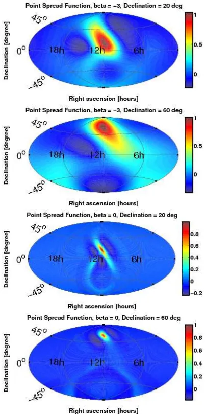
) depends strongly on the declination. FIG. 4 showsA( ˆΩ,Ωˆ′
) for different source declinations and both the β = −3 and β = 0 case, assuming continuous day coverage.
1. Scale-invariant case,β=−3
−50 0 5
1000 2000 3000 4000 5000 6000
SNR
sky area (deg
2)
S4, beta=−3 Histogram of SNR (40 bins)
Data
Ideal gaussian (sigma=1 mean=0)
[image:6.612.319.561.90.282.2]Max Likelihood: sigma=0.91836 mean=0.11816 1−sigma error for 100 indep. points
FIG. 2: S4 Result: Histogram of the signal-to-noise ratio (SNR) for β = −3. The gray curve is a maximum
likeli-hood Gaussian fit to the data. The black solid line is an ideal Gaussian, the two dash-dotted black lines indicate the expected one sigma variations around this ideal Gaussian for 100 independent points (Neff = 100).
A histogram of the SNR = Yσ is plotted in FIG. 2. The data points were weighted with the corresponding sky area in square degrees. Because neighboring points are correlated, the effective number of independent points
Neff is reduced. Therefore the histogram can exhibit statistical fluctuations that are significantly larger than those naively expected from simply counting the number of pixels in the map, while still being consistent with (cor-related) Gaussian noise. Indeed the histogram in FIG. 2 features a slight bump around SNR=2, but is still con-sistent withNeff = 100 - the red dash-dotted lines indi-cate the one sigma band around the red ideal Gaussian for Neff = 100. Additionally the SNR distribution also passes a Kolmogorov-Smirnov test forNeff = 100 at the 90% significance level.
The number of independent pointsNeff, which in effect describes the diffraction limit of the LIGO detector pair, was estimated by 2 heuristic methods:
• Spherical harmonics decomposition of the SNR map. The resulting power vsl graph shows struc-ture up to roughlyl= 9 and falls off steeply above that - the l = 9 point corresponds to one twenti-eth of the maximal power. The effective number of independent points then isNeff ≈(l+ 1)2= 100.
FIG. 2 suggests that the data is consistent with no sig-nal. Thus we calculated a Bayesian 90% upper limit for each sky direction. The prior was assumed to be flat be-tween zero and an upper cut-off set to 5×10−45Hz−1at 100 Hz, the approximate limit that can be set from just operating a single LIGO interferometer at the S4 sensi-tivity. Note, however, that this cut-off is so high that the upper limit is completely insensitive to it. Addition-ally we marginalized over the calibration uncertainty of 8% for H1 and 5% for L1 using a Gaussian probability distribution. The resulting upper limit map is shown in FIG. 6. The upper limits on the strain power spec-trum H(f) vary between 1.2×10−48Hz−1(100 Hz/f)3 and 1.2×10−47Hz−1
(100 Hz/f)3, depending on the po-sition in the sky. These strain limits correspond to limits on the gravitational wave energy flux F(f) vary-ing between 3.8×10⁻⁶erg cm−2 Hz−1(100 Hz/f) and 3.8×10⁻⁵erg cm−2 Hz−1(100 Hz/f).
2. Constant strain power, β= 0
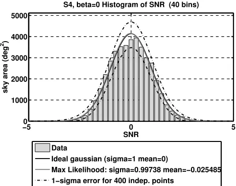
Similarly, FIG. 3 shows a histogram of the SNR = Yσ for the constant strain power case. Structure in the spherical harmonics power spectrum goes up to l = 19, thusNeff was estimated to beNeff ≈(l+ 1)2= 400. Al-ternatively the FWHM area of a strong injection covers about 100◦2 which also leads to N
eff ≈400. The dash-dotted red lines in the histogram (FIG. 3) correspond to the expected 1−σdeviations from the ideal Gaussian for
Neff = 400. The histogram is thus consistent with (cor-related) Gaussian noise, indicating that there is no signal present. The SNR distribution also passes a Kolmogorov-Smirnov test forNeff = 400 at the 90% significance level.
Again we calculated a Bayesian 90% upper limit for each sky direction, including the marginalization over the calibration uncertainty. The prior was again assumed to be flat between 0 and an upper cut-off of 5×10−45Hz−1 at 100 Hz. The resulting upper limit map is shown in FIG. 7. The upper limits on the strain power spectrum
H(f) vary between 8.5×10−49Hz−1and 6.1×10−48Hz−1 depending on the position in the sky. This corresponds to limits on the gravitational wave energy fluxF(f) varying between 2.7×10⁻⁶erg cm−2Hz−1(f /100 Hz)2
and 1.9×
10−5erg cm−2Hz−1
(f /100 Hz)2.
3. Interpretation
The maps presented in FIGS. 6 and 7 represent the first directional upper limits on a stochastic gravitational wave background ever obtained. They are consistent with no gravitational wave background being present. This search is optimized for well localized, broadband sources of gravitational waves. As such it is best suited for un-expected, poorly modeled sources.
−50 0 5
1000 2000 3000 4000 5000
SNR
sky area (deg
2)
S4, beta=0 Histogram of SNR (40 bins)
Data
Ideal gaussian (sigma=1 mean=0)
Max Likelihood: sigma=0.99738 mean=−0.025485 1−sigma error for 400 indep. points
FIG. 3: S4 Result: Histogram of the signal-to-noise ratio (SNR) forβ = 0. The gray curve is a maximum likelihood Gaussian fit to the data. The black solid line is an ideal Gaussian, the two dash-dotted black lines indicate the ex-pected one sigma variations around this ideal Gaussian for 400 independent points (Neff = 400).
In order to compare the result to what could be ex-pected from known sources we also search for the gravita-tional radiation from low-mass X-ray binaries (LMXBs). They are accretion-driven spinning neutron stars, i.e. narrow-band sources and thus not ideal for this broad-band search. However they have the advantage that we can predict the gravitational luminosity based on the known X-ray flux. If gravitational radiation provides the torque balance for LMXBs, then there is a simple relation between the gravitational luminosityLGW and X-ray lu-minosityLX [13]:
LGW ≈ fspin
fKepler
LX. (14)
Here fKepler is final orbital frequency of the accreting matter, about 2 kHz for a neutron star, andfspin is the spin frequency.
As an example we estimate the gravitational luminos-ity of all LMXBs within the Virgo galaxy cluster. Their integrated X-ray luminosity is about 10−9 erg/sec/cm2 (3000 galaxies at 15 Mpc, 1040 erg/sec/galaxy from LMXBs). For simplicity we assume that the ensemble produces a flat strain power spectrumH(f) over a band-width ∆f. Then the strength of this strain power spec-trum is about
H(f) = 2G
πc3
1
fKeplerfcenter∆f
LX
≈10−55Hz−1100 Hz
fcenter
100 Hz ∆f
.
(15)
set in this paper, which is mostly due to the fact that the intrinsically narrow-band sources are diluted over a broad frequency band.
FIG. 4: Point spread function A( ˆΩ,Ωˆ′) of the
radiome-ter for β=−3 (top two figures) and forβ= 0 (bottom two
figures). Plotted is the relative expected signal strength as-suming a source at right ascension 12hand declinations 20◦
and 60◦. Uniform day coverage was assumed, so the resulting
shapes are independent of right ascension. An Aitoff projec-tion was used to plot the whole sky.
B. Limits on isotropic background
[image:8.612.76.277.100.505.2]It is possible to recover the estimate for an isotropic background as an integral over the map (see [7]). The cor-responding theoretical standard deviation would require a double integral with essentially the point spread func-tion as integrand. In practice it is simpler to calculate this theoretical standard deviation directly by using the
FIG. 5:Injected pulsar #3: The analysis was run using the 108.625 Hz−109.125 Hz frequency band. The artificial signal
of Pulsar #3 at 108.86 Hz stands out with a signal-to-noise ratio of 9.2. The circle marks the position of the simulated pulsar.
FIG. 6: S4 Result: Map of the 90% confidence level Bayesian upper limit on Hβ for β = −3. The upper
limit varies between 1.2×10−48Hz−1(100 Hz/f)3 and 1.2×
10−47Hz−1(100 Hz/f)3
, depending on the position in the sky. All fluctuations are consistent with the expected noise.
FIG. 7: S4 Result: Map of the 90% confidence level Bayesian upper limit onHβ forβ= 0.The upper limit varies between 8.5×10−49Hz−1and 6.1×10−48Hz−1depending on
the position in the sky.
[image:8.612.317.563.263.378.2] [image:8.612.317.561.472.589.2]up-per limit we can set on h2
72Ωgw(f) is 1.20×10⁻⁴. The dimensionless quantity Ωgw(f) is the GW energy density per unit logarithmic frequency, divided by the critical energy density ρc to close the universe, and h72 is the Hubble constant in units of 72 km sec−1Mpc−1
. Table II summarizes the results for all choices ofβ.
1. Interpretation
In [1] we published an upper limit of h2
72ΩGW <
6.5×10⁻⁵on an isotropic gravitational wave background using S4 data. That analysis is mathematically identi-cal to inferring the point estimate as an integral over the map [7], but the mitigation of the timing transient and the data quality cuts were sufficiently different to affect the point estimate. While both results are consistent within the error bar of the measurement, this difference results in a slightly higher upper limit. Both results are significantly better than the previously published LIGO S3 result.
C. Narrow-band results targeted on Sco-X1
As an application we again focus on low-mass X-ray binaries (LMXBs). The gravitational wave flux from all LMXBs is expected to be dominated by the closest one, Sco-X1, simply because Sco-X1 dominates the X-ray flux from all LMXBs, and X-ray luminosityLX is related to the gravitational luminosity LGW through equation 14. Unfortunately the spin frequency of Sco-X1 is not known. We thus want to set an upper limit for each frequency bin on the RMS strain coming from the direction of Sco-X1 (RA: 16h 19m 55.0850s; Dec: -15◦
38’ 24.9”).
The binary orbital velocity of Sco-X1 is about 40±
5 km/sec (see [12]). This induces a maximal frequency shift of ∆fGW = 2.7×10⁻⁴×fGW. We chose a bin width ofdf = 0.25 Hz, which is broader than maximal frequency shift ∆fGW for all frequencies below 926 Hz and is the same bin width that was used for the broad-band analysis. Above 926 Hz the signal is guaranteed to spread over multiple bins.
To avoid contamination from the hardware-injected pulsars, the 2 frequency bins closest to a pulsar frequency were excluded. Multiples of 60 Hz were also excluded. The lowest frequency bin was at 50 Hz, the highest one at 1799.75 Hz. FIG. 8 shows a histogram of the remain-ing 6965 0.25 Hz wide frequency bins. It is consistent with a Gaussian distribution (Kolmogorov-Smirnov test withN = 6965 at the 90% significance level).
A 90% Bayesian upper limit for each frequency bin was calculated based on the point estimate and standard deviation, including a marginalization over the calibra-tion uncertainty. Figure 9 is a plot of this 90% limit (red trace). Above about 200 Hz (shot noise regime above the cavity pole) the typical upper limit rises linearly with
fre-−40 −3 −2 −1 0 1 2 3 4
100 200 300 400 500 600
SNR
N
Sco−X1, Histogram of SNR
Data
Ideal gaussian (sigma=1 mean=0)
[image:9.612.320.560.54.249.2]Max Likelihood: sigma=1.0336 mean=0.0058866 1−sigma error for 6965 indep. points
FIG. 8: S4 Result for Sco-X1: Histogram of the signal-to-noise ratio calculated for each 0.25 Hz wide frequency bin. There are no outliers.
102 103
10−24 10−23 10−22
Hz
strain
Sco−X1, ra= 16.332 h , decl= −15.6402 deg
90% Bayesian limit Standard deviation
FIG. 9: S4 Result for Sco-X1: The 90% confidence Bayesian upper limit as a function of frequency - marginalized over the calibration uncertainty. The standard deviation (one sigma error bar) is shown in blue.
quency and is given by
h(90%)RMS ≈3.4×10
−24
f
200 Hz
f >∼200 Hz. (16)
The standard deviation is also shown in blue.
1. Interpretation
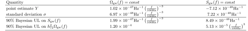
[image:9.612.320.560.308.508.2]S4 isotropic upper limit
Quantity Ωgw(f) =const Sgw(f) =const
point estimateY 1.02×10−47Hz−1`100Hzf
´−3
−7.12×10−48Hz−1
standard deviationσ 6.97×10−48Hz−1`100Hzf
´−3
7.22×10−48Hz−1
90% Bayesian UL onSgw(f) 1.99×10−47Hz−1`100Hzf
´−3
8.49×10−48Hz−1
90% Bayesian UL onh272Ωgw(f) 1.20
×10−4 5.13×10⁻⁵`100Hzf
[image:10.612.43.566.67.133.2]´3
TABLE II: S4 isotropic resultfor the Ωgw(f) =const, (β=−3) and theSgw(f) =const, (β= 0) case. The first two lines show the point estimate and standard deviation that are used to calculate the 90% Bayesian upper limits. The upper limits are also marginalized over the calibration uncertainty. These results agree with the ones published in [1] within the error bar of the measurement.
Sco-X1. Nevertheless it can set a competitive upper limit with a minimal set of assumptions on the source and significantly less computational resources. Indeed LIGO published a 95% upper limit on gravitational radiation amplitude from Sco-X1 of 1.7×10⁻²²to 1.3×10⁻²¹across the 464−484 Hz and 604−624 Hz frequency bands [4], using data from S2, which had a noise amplitude about 4.5 times higher around 500 Hz in each instrument. The analysis was computationally limited to using 6 hours of data and two 20 Hz frequency bands. However the strain amplitude sensitivity scales asT−1/4[7], while a coherent method scales asT−1/2.
The upper limit (eq. 16) can directly be compared to the expected strain based on the X-ray luminosity:
h(90%)RMS
hLX RMS
≈100
f
200 Hz 32
f >∼200 Hz. (17)
Here f is the gravitational wave frequency, i.e. twice the (unknown) spin frequency of Sco-X1. This is close enough that, if the model described in [13], and thus equation 14 are indeed correct, Sco-X1 ought to be de-tectable with this method and the next generation of gravitational wave detectors operated in a narrow-band configuration (AdvLIGO [14]). For a discussion of the expected signal from Sco-X1 see also [4].
V. CONCLUSION
We produced the first upper limit maps for a stochas-tic gravitational wave background by applying a method that is described in [7] to the data from the LIGO S4 sci-ence run. No signal was seen and upper limits were set for two different choices for the strain power spectrumH(f). In the case ofH(f)∝f−3 the upper limits for a point source vary between 1.2×10−48Hz−1(100 Hz/f)3
and 1.2×10−47Hz−1
(100 Hz/f)3, depending on the position in the sky (see FIG. 6). Similarly, in the case of constant
H(f) the upper limits vary between 8.5×10−49Hz−1and 6.1×10−48Hz−1 (see FIG. 7). As a side product limits
on an isotropic background of gravitational waves were also obtained, see TABLE II.
In an additional application, narrow-band upper lim-its were set on the gravitational radiation coming from the closest low-mass X-ray binary, Sco-X1 (see FIG. 9). In the shot noise limited frequency band (above about 200 Hz) the limits on the strain in each 0.25 Hz wide frequency bin follow roughly
h(90%)RMS ≈3.4×10
−24
f
200 Hz
f >∼200 Hz, (18)
where f is the gravitational wave frequency (twice the spin frequency).
Acknowledgments
[1] B. Abbott et al., astro-ph/0608606, to be published in ApJ.
[2] B. Abbottet al., Phys. Rev. Lett.95, 221101 (2005). [3] B. Abbottet al., Phys. Rev. D69, 122004 (2004). [4] B. Abbottet al., gr-qc/0605028, to be published in PRD. [5] B. Abbottet al., Nucl. Instrum. Methods A517(2004)
154-179.
[6] B. Allen and J.D. Romano, Phys. Rev. D 59, 102001 (1999).
[7] S.W. Ballmer, Class. Quantum Grav. 23, S179-S185 (2006).
[8] S.W. Ballmer, MIT thesis (2006).
[9] L. Bildsten, Astrophys. J. 501L89-L93 (1998)
[10] A. Lazzarini, J. Romano LIGO preprint (2004) http://www.ligo.caltech.edu/docs/T/T040089-00.pdf [11] T. Regimbau, J. A. de Freitas Pacheco Astron.
Astro-phys.376, 381 (2001)