THE DEVELOPMENT AND CALIBRATION OF A GENERIC DYNAMIC ABSORPTION CHILLER MODEL
Simon Paul Borgi, Nicolas James Kelly Energy Systems Research Unit
Department of Mechanical and Aerospace Engineering
University of Strathclyde, Glasgow, UK
ABSTRACT
Although absorption cooling has been available for many years, the technology has typically been viewed as a poorly performing alternative to vapour compression refrigeration. Rising energy prices and the requirement to improve energy-efficiency is however driving renewed interest in the technology, particularly within the context of combined cooling, heat and power systems (CCHP) for buildings. In order to understand the performance of absorption cooling, numerous models are available in the literature. However, the complexities involved in the thermodynamics of absorption chillers have so far restricted researchers to creating steady state or dynamic models reliant on data measurements of the internal chiller state, which require difficult-to-obtain, intrusive measurements. The pragmatic, yet fully-dynamic model described in this paper is designed to be easily calibrated using data obtained from the measurements of inflows and outflows to a chiller, without resorting to intrusive measurements. The model comprises a series of linked control volumes featuring both performance maps and lumped mass volumes, which reflect the underlying physical structure of the device. The model was developed for the ESP-r building simulation tool. This paper describes the modelling approach, theory and limitations, along with its calibration and the application of the model to a specific example.
1. INTRODUCTION
The increased use of air conditioning in buildings, including dwellings over the last 30 years has contributed to a significant increase in electrical energy consumption [1], particularly in southern European countries [2]. The conditioning systems installed are typically packaged, split vapour
i
Corresponding author:
compression units [3]. Due to escalating fuel costs worldwide, interest is growing in less energy intensive forms of cooling. Thermally activated absorption cooling powered either by heat absorbed by solar collectors [1, 4] or from waste heat produced by a CCHP trigeneration system [5, 6], is possibly one of the most well known and researched alternatives.
1.1 The need for a dynamic model
In order to predict model performance under fixed operating conditions steady-state models are used [7]. A number of steady-state models typically used as design aids have been developed [8-11]. However, chiller systems will typically operate under dynamic conditions, due to (for example) on/off or modulating behaviour, start-up and shut down or other temporal fluctuations in operating conditions, as discussed by Jeong et al.[12]and Fujii et al. [7]. Dynamic models [12-16], whilst intrinsically more complex, are therefore a more appropriate means to assess the performance of absorption chillers within a trigeneration system reliant on transient heat input such as that supplied by solar energy and subject to a fluctuating load.
1.2 Existing dynamic models
1.3 Requirement for a new model
The models described above typically require the user to define the characteristics of the components comprising the desired absorption chiller such as the individual components’ heat exchange surface area, individual internal component dimensions, solution composition and internal mass flow rates. This is a non-trivial task requiring invasive experimental techniques which are difficult to perform and very time-consuming; limiting the flexibility and adaptability of these models.
The scope of this research was therefore to create a functional dynamic model, which could be adapted to represent different chillers using easily obtainable data. The model concept is similar to that developed by the IEA ECBCS Annex 42 in [21] where the model of a generic engine-based CHP system was developed comprising performance maps linking key input and output parameters, coupled with lumped thermal masses that enabled transient thermal performance to be captured. The Annex 42 model was complemented by a calibration approach using non-invasive tests and measurements. The chiller model developed and described in this paper represents a single-effect hot water fed lithium bromide-water absorption chiller, the most apt [7] for use in CCHP trigeneration systems.
2. DEVELOPMENT OF THE PROPOSED MODEL
The chiller model was developed for the ESP-r building simulation tool [22] in which a complex system such as a building or a plant system can be reduced to series of discrete control volumes, represented by a node, to which the conservation of energy and mass can be applied [23]; this approach is extended to the modelling of the absorption chiller. It should be noted that the model described in this paper can be integrated into other common, dynamic simulation tools such as TRNSYS [20] or EnergyPlus [24].
2.1 The control volume concept used to model the thermal transients inside the chiller
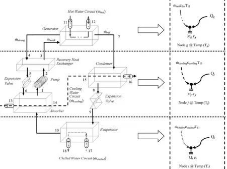
model for ESP-r.
[image:4.595.76.527.123.458.2]
Fig. 1 - The absorption chiller system represented by a system of three nodes
Applying basic energy and mass conservation individually on the three nodes, three partial differential equations, one for each node are obtained as follows:
For Node i, for an incoming chilled water flow rate ṁ having specific heat capacity
̅⁄ = ṁ− + Q,where - (1)
Q= ṁℎ− ℎ - (2)
For Node j, for an incoming cooling water flow rate ṁ having specific heat capacity
̅⁄ = ṁ !− " + Q, where - (3)
Q= ṁℎ− ℎ# + ṁℎ+ ṁ$ℎ$− ṁℎ" - (4)
For Node g, for an incoming hot water flow rate ṁ% having specific heat capacity %
̅⁄ = ṁ%% − " + &' (− " + Q, where - (5)
Q= ṁ!ℎ!− ṁ)ℎ)− ṁℎ" - (6)
The extra term UA(Tenv – Tg) in the analysis of Node g represents the heat transfer to and from the environment. The numbers in subscript refer to the individual state points within the chiller cycle as shown in Figure 1. Solving equations (1), (3) and (5) using a numerical approximation with a time interval ∆t as described in [23, 26-28] yields the temperatures of the three nodes, Ti, Tj, and Tg - the outlet temperatures of the three water circuits, the chilled, cooling and hot water circuits, respectively. In Figure 1 these are T18, T16and T12 respectively.
2.2 Finding the state points within the chiller
In order to obtain Qi, Qj and Qg, the net energy flows into and out of Node i, Node j and Node g respectively, the individual state points within the chiller’s thermodynamic cycle are calculated as follows:
Equations and assumptions used to find Qi
Q= ṁℎ− ℎ
Making the reasonable assumption that the refrigerant exits the evaporator as dry vapour, h10can be considered to be the specific enthalpy at dry conditions of plow, the low pressure inside the
evaporator-absorber. Also, assuming adiabatic expansion in the expansion valve implies that h9is equal to h8, the
specific enthalpy at wet vapour conditions of phigh, the high pressure inside the condenser-generator.
The low pressure (plow) inside the evaporator-absorber and the high pressure (phigh) inside the
condenser-generator are found based on empirically calibrated data as explained in Section 3.1. No
pressure loss is assumed to occur between the condenser and generator and similarly between the
evaporator and the absorber. The refrigerant mass flow rate, ṁ, is found using equation (7).
ṁ = *+,-⁄.1000ℎ− ℎ1 - (7)
CHPower, the chiller’s refrigerating output power is found using empirically calibrated data as described in Section 3.2.
Equations and assumptions used to find Qj
Recall from equation (4) that:
Q= ṁℎ− ℎ# + ṁℎ+ ṁ$ℎ$− ṁℎ"
Performing a mass balance analysis on the generator yields:
ṁ+ṁ2% =ṁ-34 - (8)
Assuming that all solution concentration changes occur only in the absorber and generator, the concentration in the weak and strong solution branches can be assumed to be constant such that 5= 56= 5!= 5-34 and 5)= 57= 5$= 52%, from which the circulation factor f results as shown
in equation (9).
8 = 9:;<=>? 9:;<=>?@9ABCD=
ṁABCD
The solution concentrations inside the two branches, Xstrong, and Xweak¸ are found using an iterative process which make use of a series of equations described by Kaita in [29]. In this iterative process use is made of T1, which is assumed to be slightly higher than the arithmetic mean between the inlet and outlet temperature of the cooling water circuit temperatures, T13 and T16 respectively, and T4 which is assumed to be slightly lower than the inlet temperature of the hot water circuit, T11. T1 and T4 are calculated using equation (10) and (11) respectively.
= !+ 1.275$− ! 2⁄ - (10)
)= 0.95 - (11)
Assuming solution saturation and considering the case of Xweak, the iterative process relies on comparing plow (the low cycle pressure calculated using the empirical method explained in Section 3.1)
with pweak [the low cycle pressure calculated as a function of solution concentration and temperature
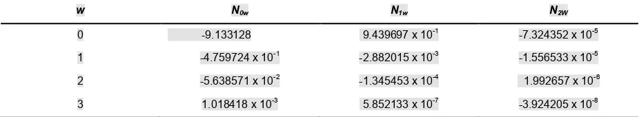
as shown in equations (12), (13) and (14)] until the two values are equal. The coefficients Nvw in equation (14) are given in Table 1 as described by Kaita in [29].
K-34= 10L,, where - (12)
MNO = 7.05 − P6!.7QR$!.7)S − P.)77T6!.7QRVUS, where D, the dew point temperature is - (13)
W = ∑ ∑! Y(-5 − 40( --[
6
[image:7.595.66.529.584.669.2]([ - (14)
Table 1 - Coefficients to calculate the dew point temperature
w N0w N1w N2W
0 -9.133128 9.439697 x 10⁻¹ -7.324352 x 10⁻⁵
1 -4.759724 x 10⁻¹ -2.882015 x 10⁻³ -1.556533 x 10⁻⁵
2 -5.638571 x 10⁻² -1.345453 x 10⁻⁴ 1.992657 x 10⁻⁶
3 1.018418 x 10⁻³ 5.852133 x 10⁻⁷ -3.924205 x 10⁻⁸
For equation (14) Tis T1 derived from equation (10), whilst Xweak is varied from an initial concentration of X being equal to 40% up to a point where pweak is equal to plow. Equation (14) is valid for a
concentrations for absorption cycle chillers and ensuring no crystallisation problems occur above 65% [30]. Similarly for Xstrong, the same iterative process is repeated this time using T4, phigh and pstrong.
Considering the solution at Point 1 and Point 6, respectively, the weak solution exiting the absorber and the strong solution entering the absorber to be saturated, the specific enthalpy of Point 1 and Point 6, h1 and h6, are calculated using the general form of equation (15) [29].
ℎ = .3.462023 − 2.679895x10@6X1 + 0.5.1.3499x10@!− 6.55x10@$X1.61 + .162.81 − 6.0418X −
4.5348x10@!X6+ 1.2053x10@!X!1 - (15)
In the case of h1, the temperature is T1 and the solution concentration is X1. On the other hand, assuming again that the expansion process in the expansion valve is completely adiabatic, h6 is equal to h5. T5 which is used to find h5 is in this case calculated using equation (16). T5 is assumed to be slightly lower than the mid-point temperature between the generator and the absorber.
7= 0.95− a0.95− - (16)
The specific enthalpy at Point 7, h7, the exit point of the refrigerant from the generator assumed to be superheated at temperature T7 and pressure phigh, is calculated using equation (17) (from Kalogirou
[31]).
ℎ= b cdeUfghigV@.!dejfghigQ6$# k@c!6.7#lm fghig"Q67!.6k"
n − # + 32.508Ln prstr" + 2513.2
- (17)
In equation (17) T8is the saturation temperature at the high cycle pressure phigh, whilst T7is calculated using equation (18); the mean temperature of the solution flows in and out of the generator [8].
cweak is the specific heat of the lithium bromide-water solution inside the weak solution branch calculated using equation (19) (from Kalogirou [31]).
-34 = 9.76u10@75-346− 3.751u10@65-34+ 3.8254 - (19)
Equations and assumptions used to find Qg
Recall from equation (6) that: Q= ṁ!ℎ!− ṁ)ℎ)− ṁℎ"
The specific enthalpy at point 4, h4, the strong solution at the exit of the generator is again found using equation (15); h3, is calculated as shown in equation (20).
ℎ!= ℎ6+ 1 − 1 8⁄ ℎ)− ℎ7 - (20)
The specific enthalpy at point 2, h2, the weak solution at the exit of the pump is calculated using equation (21).
ℎ6= ℎ+ vwxy zw{| }~ KK
= ℎ+.1145.36 + 470.84X6+ 1374.79X K− K-" 6
6 − 0.333393 + 0.571749X 6
6273 + 1
- (21)
3. MODEL CALIBRATION
The data required to calibrate the component (see Table 2) is derived from two sources:
• Some of the parameters including the highest and lowest permissible high and low pressure, the minimum chilled water protection temperature and the working minimum hot water outlet temperature can be extracted directly from manufacturer’s data sheets as these are typically listed to avoid any damage being caused to the chiller.
refrigerating power output function (CHPower) curve coefficients (d0, d1, d2 and d3), the thermal
masses (Mi, Mj and Mg) and the mass weighted average specific heat values (, and c t) all require empirical data, obtained from a three stage calibration process. Details on how these values can be obtained are given in Sections 3.1, 3.2 and 3.3.
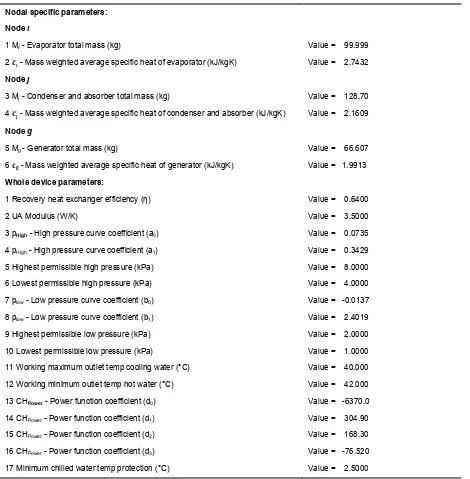
[image:10.595.67.537.291.770.2]Table 2 lists the parameters that require calibration together with the respective values obtained after calibrating the model with experimentally measured data acquired for a 10 kWth absorption chiller developed by SK SonnenKlima GMbH[32, 33].
Table 2 - Component coefficients and data describing the absorption chiller plant component
Nodal specific parameters: Node i
1 Mi - Evaporator total mass (kg) Value = 99.999
2 - Mass weighted average specific heat of evaporator (kJ/kgK) Value = 2.7432
Node j
3 Mj - Condenser and absorber total mass (kg) Value = 128.70
4 - Mass weighted average specific heat of condenser and absorber (kJ/kgK) Value = 2.1609
Node g
5 Mg - Generator total mass (kg) Value = 66.607
6 ̅ - Mass weighted average specific heat of generator (kJ/kgK) Value = 1.9913
Whole device parameters:
1 Recovery heat exchanger efficiency (ƞ) Value = 0.6400
2 UA Modulus (W/K) Value = 3.5000
3 pHigh - High pressure curve coefficient (a0) Value = 0.0735
4 pHigh - High pressure curve coefficient (a1) Value = 0.3429
5 Highest permissible high pressure (kPa) Value = 8.0000
6 Lowest permissible high pressure (kPa) Value = 4.0000
7 plow - Low pressure curve coefficient (b0) Value = -0.0137
8 plow - Low pressure curve coefficient (b1) Value = 2.4019
9 Highest permissible low pressure (kPa) Value = 2.0000
10 Lowest permissible low pressure (kPa) Value = 1.0000
11 Working maximum outlet temp cooling water (°C) Value = 40.000
12 Working minimum outlet temp hot water (°C) Value = 42.000
13 CHPower - Power function coefficient (d0) Value = -6370.0
14 CHPower - Power function coefficient (d1) Value = 304.90
15 CHPower - Power function coefficient (d2) Value = 168.30
16 CHPower - Power function coefficient (d3) Value = -76.520
18 Circulation pump electrical efficiency (-) Value = 0.9000
Control variables:
1 ‘On’/‘Off’ Control signal (-) Value = 1/0
3.1 Cycle high and low pressures in terms of the hot water circuit inlet temperature
This section explains how the general relationships between the internal high (phigh) and low (plow)
cycle pressures and the incoming inlet temperature of the hot water circuit were obtained and how the pressure curve coefficients (a0, a1, b0 and b1) were eventually calibrated.
3.1.1 Calibration 1: Obtaining the cycle high and low pressures in terms of the hot water circuit inlet temperature
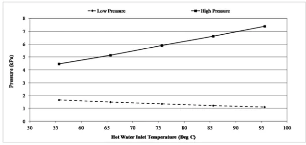
[image:11.595.145.449.602.746.2]Experimental data obtained from the IEA Task 38 Solar Heating and Cooling Programme (personal communication, October 29, 2010) for the mentioned 10 kWth absorption chiller shows that over the working range of inlet water circuit temperatures (lowest and highest hot water temperature working range [55-95°C - 40°C], lowest and highest cooling water temperature working range [35-27°C - 7°C] and lowest and highest chilled water temperature working range [20-6°C - 14°C]) [32], both the high pressure inside the condenser-generator and the low pressure inside the evaporator-absorber are predominantly effected by the hot water circuit inlet temperature, and that the inlet temperatures of the cooling and chilled water flow circuits have only a marginal effect on the cycle pressures. Also, the control scheme employed by most chillers is to use constant water circuit flow rates and use the hot or cooling water inlet circuit temperature to control the output power of the absorption chiller [34]. Considering these conditions, a reasonable assumption is therefore that the cycle pressures can be modelled as a function of hot water circuit inlet temperature.
The experimental data of Figure 2 shows how the high pressure inside the condenser-generator and the low pressure inside the evaporator-absorber vary over the whole range of hot water circuit inlet temperatures. Both the high pressure inside the condenser-generator and the low pressure inside the evaporator-absorber vary linearly with change in hot water circuit inlet temperature. However, whereas the pressure inside the condenser-generator increases with increasing temperature, the pressure inside the evaporator-absorber decreases with increasing temperature.
The high and low cycle pressure curves coefficients (a0, a1, b0 and b1) can therefore be derived by
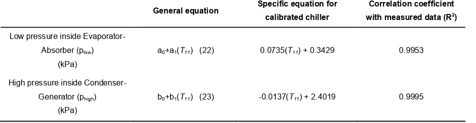
[image:12.595.66.539.462.585.2]varying the hot water circuit inlet temperature to the generator and recording the resulting part-load cycle pressures. A similar calibration exercise can be repeated to obtain the characteristics of any other chiller. The relationships describing the behaviour of the two system pressures with a corresponding change in T11, the hot water circuit inlet temperature in °C, were obtained using a linear regression analysis on the test data shown in Figure 2. Table 3 shows the general and particular equations for the calibrated chiller together with the corresponding correlation coefficients.
Table 3 - Relationships between hot water inlet temperature and the high and low pressure
General equation Specific equation for calibrated chiller
Correlation coefficient with measured data (R2)
Low pressure inside
Evaporator-Absorber (plow)
(kPa)
a0+a1(T11) (22) 0.0735(T11) + 0.3429 0.9953
High pressure inside
Condenser-Generator (phigh)
(kPa)
b0+b1(T11) (23) -0.0137(T11) + 2.4019 0.9995
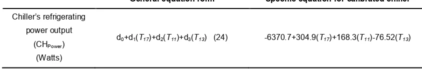
3.2 Calibration 2: Obtaining the chiller’s refrigerating power output as a function of water circuits’ inlet temperatures
all other internal mass flow rates are calculated. Similarly to the regression analysis performed in the previous section, the expression considers the case that the flow rates of all three incoming water circuits (hot, chilled and cooling water circuits) remain constant, whilst temperature can vary.
[image:13.595.83.505.375.444.2]The calibration used a time-series dataset compiled from three non-consecutive days during which the absorption chiller was being field tested together with a solar water heating system. This is similar to the approach employed by Ferguson et al. in [35]. Data was supplied in the form of 1-minute averaged recordings of the three water circuits’ individual inlet and outlet temperatures and their respective mass flow rates. The chiller’s refrigerating power output can be expressed in terms of the three water circuits’ inlet temperatures - the best fit being a simple linear relation having the general form of equation (24) shown in Table 4.
Table 4 - Relationship between the chiller’s refrigerating power output and the water circuits’ inlet temperatures
General equation form Specific equation for calibrated chiller
Chiller’s refrigerating
power output
(CHPower)
(Watts)
d0+d1(T17)+d2(T11)+d3(T13) (24) -6370.7+304.9(T17)+168.3(T11)-76.52(T13)
Where T11 is the hot water circuit inlet temperature, T13 is the cooling water circuit inlet temperature and T17 is the chilled water circuit inlet temperature. The coefficient values (d0, d1, d2 and d3) can be
calibrated for any kind of single-effect lithium bromide-water chiller using a similar dynamic dataset obtained from experimental measurements.
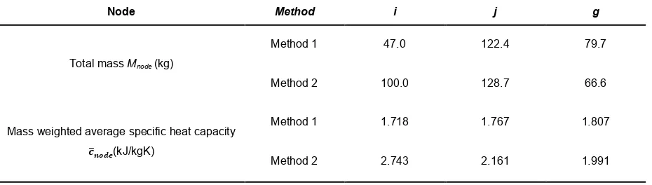
3.3 Calibration 3: Obtaining the total mass and the mass weighted average specific heat capacity of each individual node
each individual node can simply be considered as the mathematical addition of all the masses (m1, m2,.;, mn) represented by the node as shown in equation (25). The mass weighted average specific heat capacity (̅) is on the other hand, the specific heat of the node calculated using the specific heat values of the components making up an individual node (c1, c2,;., cn) as shown in equation (26).
= + 6+ ⋯ + - (25)
̅ = + 66+ ⋯ + ⁄ + 6+ ⋯ + - (26)
For this specific 10kWth chiller Kohlenbach in [34] gives a detailed breakdown of the masses and characteristics of the individual internal components from which Mnode and ̅ can be calculated as shown in Table 5. Using such a method however suffers from two major limitations. As discussed previously a first limitation is of course the fact that detailed data is required for the internal components of the chiller. This data may not be available or require intrusive measurements to obtain. An additional limitation is the fact that, in a complex plant system such as an absorption chiller where a considerable part of the mass (approx. 21% of the total mass) is water being moved along the plant component, it is difficult to accurately assign individual mass components to the individual nodes.
To address these two limitations the proposed model permits a second method of calibration which relies completely on an iterative parametric identification process, which makes use of an optimization tool; this drives the simulation over multiple runs, comparing the modelled outlet temperatures of the three water circuits with the measured outlet water data for the same feed conditions. For each run the thermal masses (Mi, Mj and Mg) and the mass weighted average specific heat values (, and c t) are varied individually and the resulting error between the modelled and the measured outlet water temperatures computed. The values of the thermal masses and the mass weighted average specific heat values which best represent the internal dynamics of the chiller are obtained once the error, which in this case is the objective function, is minimised. This is similar to the parametric identification technique described in by Ferguson et al. in [35].
average specific heat values (, and c t) obtained using both methods; Method 1 using the known data of the characteristics of the internal components and Method 2 using the iterative process.
Table 5 - Mnodeand ̅ calculated using both methods
Node Method i j g
Total mass Mnode (kg)
Method 1 47.0 122.4 79.7
Method 2 100.0 128.7 66.6
Mass weighted average specific heat capacity
(kJ/kgK)
Method 1 1.718 1.767 1.807
Method 2 2.743 2.161 1.991
Although the two set of results appear to be substantially different from one another, in practice, when modelling the dynamic output of the proposed chiller, the difference is negligible. Figure 3 (for example) shows the resulting temperature profile for the chilled water circuit using the thermal masses and the mass weighted average specific heat values calculated using both methods.
Fig. 3 - Chilled water circuit outlet temperature response
The two sets give very similar results with an average error calculated over the investigated period shown in Figure 3, between the modelled and measured data of 0.27°C in the case of Method 1, and 0.21°C in the case of Method 2.
4. VERIFICATION - MODEL TESTING AND COMPARISON BETWEEN MEASURED AND MODELLED DATA
[image:15.595.150.451.428.566.2]• an inter-model comparative exercise where the results obtained for the proposed chiller were compared to results obtained from the model presented by Kohlenbach and Ziegler in [13, 16], which was calibrated against the same 10 kWth chiller; and
• the model was compared to a separate set of experimental results compared to that used for calibration purposes.
4.1 Inter-model comparison
Kohlenbach and Ziegler in [13, 16] performed a dynamic test on their model whereby it was first run at steady-state conditions at rated inlet temperatures and mass flow rates and then subjected to a 10°C step increase in hot water circuit inlet temperature. The results obtained in this experiment indicated that it took around 10-minutes for the hot water temperature to stabilise at the new state, and approximately 15-minutes for the remaining chiller parameters to reach steady-state, depending on the thermal mass involved in each internal component. Replicating this test using the dynamic model, the chiller was supplied at steady, rated conditions (hot water circuit inlet temperature of 75°C with a mass flow rate of 0.4kg/s, chilled water circuit inlet temperature of 18°C with a mass flow rate of 0.8kg/s and the cooling water circuit inlet temperature of 27°C with a mass flow rate of 0.7kg/s). A step increase of 10°C was then applied to the hot water circuit inlet temperature. The simulation was run at a resolution of 1 second. The results obtained for the proposed model are very close to those reported by Kohlenbach and Ziegler, with the simulated hot water circuit outlet temperature modelled stabilising in 620 seconds. The Kohlenbach and Ziegler model reached a stable state at around 600 seconds; this is a difference of around 3%.
4.2 Comparison with experimental data
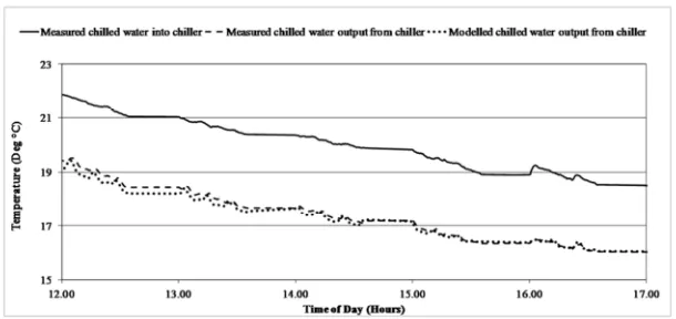
The chiller was supplied with minute by minute inlet temperature measurements of the three water circuits entering the chiller from an empirical data set. The resulting set of simulated output temperatures was then compared to the measured data.
at 1-minute time resolution, along with the measured chilled water inlet and outlet temperatures data. The modelled data closely follows the measured data with identical time response patterns, yielding a maximum and mean error of 0.35°C and 0.09°C between the modelled and measured datasets, respectively. The standard deviation is 0.10°C.
Fig. 4 - Measured vs. modelled chilled water data
[image:17.595.146.456.481.650.2]Figure 5, shows how the modelled data smoothed to give a weighted value to any possible outliers compares to an ideal fit. The modelled data again closely follows the ideal fit resulting in a correlation coefficient value of 0.995.
Fig. 5 - Modelled chilled water circuit outlet temperature data vs. ideal fit
Fig. 6 - Measured vs. modelled cooling water datasets
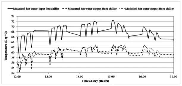
Fig. 7 - Measured vs. modelled hot water datasets
Both figures show good agreement between the measured and modelled datasets, although showing a slightly positive temperature bias when compared to the results obtained from the chilled water. In terms of the cooling water circuit temperatures, the maximum and mean error values between the modelled and measured datasets were calculated to be 2.19°C and 0.22°C respectively. The calculated standard deviation was 0.61°C. The hot water circuit temperatures showed a similar behaviour to the cooling water temperatures with the maximum and mean error values between the modelled and measured datasets being 2.81°C and 0.46°C respectively, whilst the standard deviation was calculated to be 0.93°C.
5. PERFORMANCE INSIDE A MICRO-TRIGENERATION SYSTEM
[image:18.595.146.452.284.429.2]obtained during the testing of the chiller model inside a micro-trigeneration fed centralised heating, ventilation and air conditioning (HVAC) system for a three storey residential building in the Mediterranean island of Malta. The analysis forms part of an extensive research aimed at understanding the effect certain building (e.g. the building fabric, size and occupancy and the electrical demand) and plant related features (e.g. addition of a chilled water storage tank and the addition of a solar water heating working in tandem with the CHP unit) have on a residential micro-trigeneration system’s energetic, environmental and economic performance.
Compared to the relatively stable electrical and thermal demands typical of large buildings, residential buildings have a very variable and time-dependant demand. Simulations performed at low resolutions (e.g. hours) are therefore not accurate enough when performing simulations of a highly varying environment such as that found in residential buildings and therefore typically a high temporal resolution of 1 minute is preferred [36]. The varying nature and the high temporal resolution required in this case necessitate the use of a dynamic compared to steady-state absorption chiller model.
5.1 Micro-trigeneration plant configuration
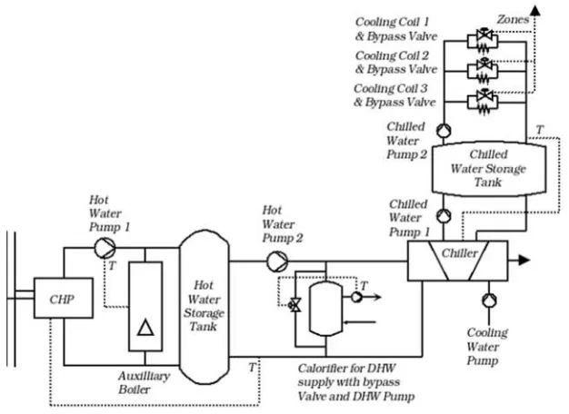
[image:19.595.142.455.506.734.2]Figure 8 shows the specific micro-trigeneration system plant configuration used to simulate a plant system which includes a chilled water storage tank.
The system model consists of a 5 kWel CHP unit (and an auxiliary boiler) feeding a 500 litre hot water buffer tank which then feeds both the domestic hot water tank and the absorption chiller. Hot water pump 2 runs at a constant flow rate of 0.8kg/s and its feed is equally divided between the domestic hot water tank and the chiller. The chiller feeds the chilled water storage tank with chilled water, whilst the cooling coils inside the ventilation system are fed chilled water from the chilled water storage tank. Both chilled water pumps run at a constant flow rate of 0.4kg/s. The chiller is controlled via a temperature sensor-actuator control scheme which senses the return temperature of the chilled water flowing back from the cooling coils into the storage tank. This sensor-actuator control scheme ensures that the chiller maintains the temperature inside the chilled water tank between 6°C and 12°C. The ventilation cooling coils are connected individually to each floor (one cooling coil for each floor), and each is individually controlled during specific hours of the day to keep the indoor temperature between 21°C and 24°C. The cooling load supplied by each individual coil is controlled by varying the amount of chilled water flowing inside the cooling coils through the use of bypass valves.
5.2 Results and performance - Chiller’s thermal and operating performance
[image:20.595.83.507.449.743.2]Figure 9 and Figure 10 show extracts from the results obtained for a simulation run at 1-minute intervals over a period of a whole week in August, using the plant system configuration shown in Figure 8. Specifically Figure 9 shows the inlet and outlet temperatures of the different water streams, whilst Figure 10 shows the corresponding refrigerating power produced by the Chiller in response to the building cooling demand, over the same time period. The time period shown in both figures is for a typical 12-hour period.
[image:20.595.146.455.602.745.2]Fig. 10 - Refrigerating power produced by Chiller
The triangular oscillations in both temperature and refrigerating power produced are in response to the control imposed on the CHP unit, which cycles ‘On’ and ‘Off’ to maintain the hot water temperature inside the hot water storage tank between 65°C and 75°C. The chiller’s output power is responsive to the temperature change in hot water supply, and in other plant configurations, the output power can be controlled via the hot or cooling water inlet temperature as discussed by Kohlenbach in [34]. In this example however the plant system control scheme was kept simple and the chiller was controlled by a simple ‘On’/‘Off’ control scheme similar to the one used to control the CHP unit.
Also, the chiller’s thermal performance is responsive to the thermal demand of the building; switching ‘On’/‘Off’ is most frequent when the cooling demand is low whilst the system works with a more stable behaviour as the building thermal demand increases. The chilled water storage tank acts as a buffer between the refrigerating power produced by the chiller and the space cooling demand of the building.
5.3 Results and performance - Seasonal system performance
duration of the cooling season. As explained the simulations were run at 1-minute resolution, with the results then aggregated on a seasonal basis. The results highlight the energetic and operational performance of the micro-trigeneration system for the cooling season, when the absorption chiller model was used to provide space cooling to the building.
Table 6 - Seasonalperformance metrics for the proposed micro-trigeneration system
Performance Metric Value Comment
Chiller seasonal operational time
(Hours)
1,735 Total number of hours chiller was ‘On’
Chiller seasonal operational load factor
(%)
59.3 Percentage time chiller was ‘On’ compared to the total possible time (June - September/122 Days/2,928 Hours)
Space cooling energy provided
(kWh)
10,982 Total space cooling energy delivered to the entire building for the period examined
Electricity cogenerated
(kWh)
14,427 Total electricity cogenerated by the CHP unit; partly exported to the grid and partly used to satisfy own demand
Energy supplied to provide domestic hot
water
(kWh)
2,342
Total energy supplied to heat water from mains temperature to
approx. 60-65°C. Daily average water consumption assumed of
30litre/person/day.
Fuel supplied to CHP unit and auxiliary
boiler
(kg LPG)
2,357 Total fuel supplied to system; the CHP unit and auxiliary boiler. Fuel used was Liquefied Petroleum Gas (LPG)
Micro-trigeneration primary energy
consumption
(kWh)
31,214 Assumes a calorific value for LPG of 46.15 MJ/kg [37]
Micro-trigeneration system efficiency
(%)
69.1
Overall system efficiency is based on equation by Dorer in [38]
which compares the energy products produced by the
micro-trigeneration system:
• Space cooling energy provided;
• Electricity cogenerated; and
• Energy supplied to provide domestic hot water
to the energy input of the system (Micro-trigeneration primary
energy consumption)
6. CONCLUSION
require re-calibration of the internal components in order to represent different chiller types, the model presented in this research can be calibrated simply by measured data of the inlet and exit temperatures of the three water circuits flowing in and out of the chiller. The model is therefore very flexible and adaptable for calibration with other similar chillers. The model predictions were compared to an alternative model and to measured data showing good agreement with both. Finally, an application of the model is presented demonstrating the kind of performance metrics that can be extracted using a dynamic chiller model.
NOMENCLATURE Variables
A Area (m2)
̅ Mass weighted average specific heat capacity (kJ/kgK)
c Specific heat (kJ/kgK) f Circulation ratio (-) h Specific enthalpy (kJ/kg) M Total mass of node (kg) ṁ Mass flow rate (kg/s)
m Mass of component inside the chiller (kg) p Cycle pressure (kPa)
t Time (sec)
T Temperature (°C)
U Component total heat loss coefficient (W/m2K) X Solution concentration of lithium bromide in water (%) Greek Letters
ƞ Recovery heat exchanger effectiveness Indices
chilled Chilled water flow circuit cooling Cooling water flow circuit
el Electrical power
g Internal node within the absorption chiller representing the thermal mass which is associated with the hot water circuit
high High pressure of absorption refrigeration cycle found in generator-condenser hot Hot water flow circuit
i Internal node within the absorption chiller representing the thermal mass which is associated with the chilled water circuit
j Internal node within the absorption chiller representing the thermal mass which is associated with the cooling water circuit
low Low pressure of absorption refrigeration cycle found in absorber-evaporator
ref Refrigerant
strong Chiller branch with the strong solution th Thermal power
weak Chiller branch with the weak solution
ACKNOWLEDGMENTS
The research work disclosed in this publication is partially funded by the Strategic Educational Pathways Scholarship (Malta). The scholarship is part-financed by the European Union – European Social Fund (ESF) under Operational Programme II – Cohesion Policy 2007-2013, “Empowering People for More Jobs and a Better Quality of Life”. The authors would also like to thank members of the IEA Task 38 Solar Heating and Cooling Programme for providing the necessary data to calibrate the model.
REFERENCES
[1] C. Monné, et al., "Monitoring and simulation of an existing solar powered absorption cooling system in Zaragoza (Spain)" Applied Thermal Engineering, 2011. 31: pgs. 28-35
[2] Almeida, A.d., et al. (2008). "Final Report REMODECE - Residential monitoring to Decrease Energy use and Carbon Emissions in Europe (IEEA Program Funded Project)" - Department of Electrical Engineering, University of Coimbra. Portugal. Available from:
http://www.isr.uc.pt/~remodece/downloads/REMODECE_D9_Nov2008_Final.pdf
results from a study on room air conditioner energy efficiency" in ACEEE Summer Study on Energy Efficiency in Buildings. 2000. Washington D.C, USA
[4] S.A. Kalogirou, et al., "Modelling and simulation of an absorption solar cooling system for Cyprus" Solar Energy 2002. 72(1): pgs. 43-51
[5] Khatri, K.K., et al., "Experimental investigation of CI engine operated micro-trigeneration system" Applied Thermal Engineering, 2010. 30: pgs. 1505-1509
[6] Wang, R.Z., X.Q. Kong, and X.H. Huang, "Energy efficiency and economic feasibility of CCHP driven by stirling engine" Energy Conversion and Management 2004. 45: pgs. 1433-1442
[7] T. Fujii, et al., "Dynamic simulation program with object-oriented formulation for absorption chillers (modelling, verification, and application to triple-effect absorption chiller)" International Journal of Refrigeration 2010. 33: pgs. 259-268
[8] M A Mehrabian and A.E. Shahbeik, "Thermodynamic modelling of a single-effect LiBr–H2O absorption refrigeration cycle" Proc. IMechE, 2004. 219(Part E)
[9] J. M. Gordon and K. Choon Ng, "A general thermodynamic model for absorption chiller: Theory and experiment" Heat Recovery Systems and CHP, 1995. 15(1): pgs. 77-83
[10] K.C. Ng, et al., "Theoretical and experimental analysis of an absorption chiller" International Journal of Refrigeration, 1993. 17(5): pgs. 351-358
[11] G. Grossman and A. Zaltash, "ABSIM - Modular Simulation of Absorption Systems" International Journal of Refrigeration, 2001. 24: pgs. 531-543
[12] S. Jeong, B.H. Kang, and S.W. Karngt, "Dynamic simulation of an absorption heat pump for recovering low grade heat" Applied Thermal Engineering, 1998. 18(1-2): pgs. 1-12
[13] Kohlenbach, P. and F. Ziegler, "A dynamic simulation model for transient absorption chiller performance. Part II: Numerical results and experimental verification" International Journal of Refrigeration, 2008. 31: pgs. 226-233
[14] Y. Takagi, T. Nakamaru, and Y. Nishitani, "An Absorption chiller model for HVACSIM+", in IBPSA Conference 1999. Kyoto, Japan
[16] Kohlenbach, P. and F. Ziegler, "A dynamic simulation model for transient absorption chiller performance. Part I: The model" International Journal of Refrigeration, 2008. 31: pgs. 217-225 [17] Witte, K.T., et al., "Absorption chiller modelling with TRNSYS - requirements and adaptation to the machine EAW Wegracal SE 15 - requirements and adaptation to the machine EAW
Wegracal SE 15", in EUROSUN 2008 - 1st International Congress on Heating and Cooling in Buildings. 2008: Lisbon, Portugal
[18] Maria Puig-Arnavat, et al., "Analysis and parameter identification for characteristic equations of single and double-effect absorption chillers by means of multivariable regression"
International Journal of Refrigeration, 2010. 33: pgs. 70-78
[19] Nurzia, G., (2008) "Design and simulation of solar absorption cooling systems." - Dipartimento di Ingegneria Industriale, Facoltà di Ingegneria, Università degli Studi di Bergamo, Italia [20] "TRNSYS - A TRaNsient SYstem Simulation Program", 2004, Solar Energy Laboratory,
University of Wisconsin-Madison, USA
[21] Beausoleil-Morrison, I., et al. (2007). "Specifications for Modelling Fuel Cell and Combustion-Based Residential Cogeneration Devices within Whole-Building Simulation Programs - A
Report of Subtask B of FC+COGEN-SIM The Simulation of Building-Integrated Fuel Cell and
Other Cogeneration Systems" - www.cogen-sim.net
[22] "ESP-r", 2005, Energy Systems Research Unit, Department of Mechanical and Aerospace Engineering, University of Strathclyde, Glasgow, UK
[23] Clarke, J.A., "Energy simulation in building design". 2nd Edition ed. 2001, Oxford: Reed Educational and Professional Publishing Ltd.
[24] "EnergyPlus", 1996, US Department of Energy, USA
[25] Ian Beausoleil-Morrison, et al. "The simulation of a residential space-cooling system powered by the thermal output of a cogeneration system" in Proceedings of esim 2004. Vancouver, Canada: IBPSA-Canada
[26] Hensen, J.L.M., (1991) "On the thermal Interaction of building structure and heating and ventilation system." PhD Thesis - Technische Universiteit Eindhoven, The Netherlands [27] Kelly, N.J., (1998) "Towards a design environment for building integrated energy systems:
UK
[28] Aasem, E.O., (1993) "Practical simulation of buildings and air-conditioning in the transient domain." PhD Thesis - Department of Mechanical and Aerospace Engineering, University of Strathclyde, Glasgow, UK
[29] Kaita, Y., "Thermodynamic properties of lithium bromide-water solutions at high temperatures" International Journal of Refrigeration, 2001. 24: pgs. 374-390
[30] S.A.Klein, R. Radermacher, and K.E. Herold, "Chapter 6 - Single Effect Water/Lithium Bromide Systems", in Absorption Chillers and Heat Pumps. 1996, CRC Press: New York, USA
[31] S.A. Kalogirou, et al., "Design and construction of a LiBr-water absorption machine" Energy Conversion and Management, 2003. 44: pgs. 2483-2508
[32] Clauβ, V. "Sonnenklima Suninverse - Solar cooling product information and experience" in Derbi Conference. 2009. Perpignan, France
[33] SONNENKLIMA package solution description, Accessed: 26/11/2010, Available from:
http://www.solarcombiplus.eu/NR/rdonlyres/AE4C63BB-CF2E-4A45-8D93-94C44A410ECC/0/D46_SonnenKlima_v02_English.pdf
[34] Kohlenbach, P., (2006) "Solar cooling with absorption chillers: Control strategies and transient chiller performance." Doctoral Thesis - Von der Fakultät III – Prozesswissenschaften, Technischen Universität Berlin, Germany
[35] Ferguson, A., et al. (2007). "Inter-Model Comparative Testing and Empirical Validation of Annex 42 Models for Residential Cogeneration Devices - A Report of Subtask B of
FC+COGEN-SIM The Simulation of Building-Integrated Fuel Cell and Other Cogeneration
Systems" - www.cogen-sim.net
[36] Stokes, M., (2004) "Removing barriers to embedded generation: a fine-grained load model to support low voltage network performance analysis." Doctoral Thesis - Institute of Energy and Sustainable Development, De Montfort University, Leicester, UK
[37] International Energy Agency, "Energy Statistics Manual", ed. Claude Mandil. 2004, Paris, France