A new maximum power point tracking technique for permanent magnet synchronous generator based wind energy conversion system

A New Maximum Power Point Tracking

Technique for Permanent Magnet

Synchronous Generator Based Wind

Energy Conversion System

Yuanye Xia+, Khaled H. Ahmed*, Barry W. Williams+ Organization:

+Department of Electronic and Electrical Engineering, Strathclyde University, Glasgow, UK

*Electrical Engineering Department, Faculty of Engineering, Alexandria University, Alexandria, Egypt.

Corresponding author: Yuanye Xia

Email: [email protected] Address:

Royal College Building, 204 George Street, Glasgow, G1 1XW

Keywords: MPPT, PMSG, power coefficient, wind energy

Abstract: A new maximum power point tracking technique for permanent magnet

pre-knowledge of a system, but has an accurate and fast response to wind speed fluctuations. Moreover, it has the ability of online updating of time-dependant turbine or generator parameter shift. The validity and performance of the proposed technique is confirmed by MATLAB/Simulink simulations and experimentations.

I. Introduction

The demand for electricity power is growing rapidly and is expected to keep growing. According to the Energy Information Administration (EIA) in the U.S., from 1990 to 2007, growth in net electricity generation outpaced the growth in total energy consumption. Meanwhile, it is estimated that the world net electricity generation will increase by 87% in the Reference case, from 18.8 trillion kilowatt-hours in 2007 to 35.2 trillion kilowatt-hours in 2035, at an average annual rate of 2.3% [1]. Due to escalating oil prices and CO2 emission reduction demand, renewable energy,

especially wind energy, becomes more and more attractive and competitive.

Wind energy can be captured and transformed to electric energy using a wind turbine and electric generator. Due to wind energy and turbine features, optimum wind energy extraction can be achieved by operating the wind turbine in a variable-speed mode. At a given wind speed, the efficiency is drastically affected by the turbine’s tip speed

Cp-max

opt

Fig.1. A typical power coefficient curve

A maximum power point tracking (MPPT) algorithm increases the power conversion efficiency by regulating the turbine rotor speed according to actual wind speeds. Therefore an effective and low implementation cost MPPT algorithm is essential to enhance the efficiency and economics of wind energy conversion systems (WECS).

Basically there are three types of MPPT algorithms, namely, tip speed ratio (TSR) control, perturb and observe (P&O) control (which is also known as hill-climbing searching (HCS) control), and optimum relationship based (ORB) control [3][4].

anemometer is expensive and adds extra cost to the system, especially for small scale WECSs. Moreover, it presents a number of difficulties in practical implementation. For example, the wind velocity close to the turbine is different from the free stream velocity [10], and due to gust and turbulence, extra processing of the wind speed measurement must be incorporated. Furthermore, the optimum TSR is dependent on the system characteristics and should be obtained in advance.

ORB control assures MPPT with the aid of knowledge of optimum relationships between system parameters [18]-[31]. Wind speed measurement is not required and the response to wind speed change is fast. Therefore it is a mature technique for applications of different power ratings. The power versus rotor speed relationship is used in [18]-[23][41], and the power versus rectifier dc voltage relationship is used in [24]. These control strategies are also known as power signal feedback control [3]. Other optimum relationships not including a power signal have also been proposed. In [23][25]-[28], the relationship between electrical torque and rotor speed is employed to track MPP. In order to further simplify control, rectifier dc voltage versus dc current relationship is used in [23][29]-[31]. Although ORB control is widely used in wind WECSs, the main drawback is that system pre-knowledge is required, which varies from one system to the other. The knowledge is obtained via simulation and lab tests, and should be further corrected by field tests. Moreover, parameter shift caused by the system aging may affect MPPT efficiency. Additionally, ORB control may consume a lot of memory space [32].

An alternative method for MPPT is proposed in [3]. A microcontroller is utilized to save the optimum power versus dc voltage relationship obtained by P&O control. No anemometer is required and it is suitable for large inertia systems. However, significant off-line experimentation is required as the maximum power points for every dc voltage value need to be tested and recorded. In [31], the authors proposed a method to find the optimum relationship between voltage and current, by obtaining one voltage and current pair, (Vdc, Idc), of the relationship first, using normal P&O

implemented assuming steady wind conditions, therefore impractical in actual application.

In this paper, a new MPPT technique combining P&O and ORB control, for permanent magnet synchronous generator (PMSG) based WECSs, is proposed. It does not need an anemometer or system pre-knowledge. The optimum relationship between rectified dc voltage and current [23][29]-[31] is rapidly obtained by advanced P&O control. Then the system is controlled using conventional ORB control. Unlike the method proposed in [3], no off-line experiments are required and the accurate optimum relationship can be rapidly obtained in variable wind conditions. Its validity is confirmed by MATLAB/Simulink simulations.

The paper is organized in seven sections. Section I introduces the conventional MPPT methods. In section II, the system configuration for investigation is presented. Section III describes the characteristic of WECS and establishes the effectiveness of the optimum relationship of rectified dc voltage and current for MPPT. In section IV, a new MPPT technique is proposed, and presented in details. The simulation results demonstrate the validity of the new technique in section V. Experimental implementation to verify the proposed technique is represented in section VI. Section VII discusses the extension of the technique to other topologies and systems.

II. System configuration

or the maximum turbine rotor speed is reached [42][43]. Because the PMSG has a high efficiency and does not require for a gear box and external excitation current, it is favoured in WECS [34]. The output power transfers through an AC-DC-AC stage, which consists of a diode bridge rectifier, a boost converter, and a grid-side inverter, which is connected to the grid. Due to the low cost and high reliability of diode bridge rectifier, it is employed instead of a controlled rectifier. A boost converter controls the dc side voltage and current for MPPT, and steps up the voltage for grid connection. Finally, the captured power is transferred to the grid via an inverter. The scheme in Fig.2 is used in this paper to demonstrate the validity of the new MPPT technique because of its simplicity and clarity.

PMSG Grid

Diode

Rectifier Grid-side

Inverter DC link

Boost Converter dc

i

dc

v

Fig.2 A normal wind energy conversion system

III. Wind energy conversion system characteristics

A. Mechanical characteristics

The energy derived from wind by the wind turbine is expressed as [35]

𝑃 = 1

2𝜌𝐶𝑝𝐴𝑣𝑤

3 ₍₁₎

where  is the air density, A is the wind turbine swept area, vw is the wind speed and

Cp is the power coefficient. Cp is a nonlinear function of tip speed ratio, , if the

turbine pitch angle is fixed. is defined as

𝜆 =𝑟Ω

where r is the rotor radius, Ω is the turbine rotor speed. A typical Cp- curve is shown

in Fig.1. There is an optimum opt, at which the power efficient is maximum. Cp-max

are fixed values for a given wind turbine.

From equation (1) and (2), it can be concluded that

𝑃_𝑚𝑎𝑥 ∝ 𝑣_𝑤3 ∝Ω_𝑜𝑝𝑡3

(3)

where Ωopt is the optimum rotor speed at a given wind speed.

B. Electrical characteristics

For a PMSG with a constant flux, the phase back electromotive force, E, is a linear function of generator rotor speed [36], which equals the turbine rotor speed,

𝐸 = 𝐾𝑒ΦΩ (4)

where Ф is the generator flux and Ke is a coefficient.

The phase terminal voltage function for a non-salient PMSG is written as

𝑉𝑎𝑐 = 𝐸 − 𝐼𝑎𝑐(𝑅𝑠+ 𝑗Ω𝑒𝐿𝑠) (5)

Ω_𝑒 = 𝑝Ω

where Vac is the phase terminal voltage, Iac is the phase current, Rs is the stator

resistance, Ls is the stator inductance, Ωe is electrical angular frequency, and p is the

number of pole pairs.

Due to the diode bridge rectifier, the ac side voltage amplitude Vac-amp and dc side

voltage Vdc can be expressed as [37]

𝑉𝑑𝑐= 3√3_𝜋 𝑉𝑎𝑐−𝑎𝑚𝑝 (6)

From equations (4) to (6), there is the approximate relationship

𝑉_𝑑𝑐 ∝Ω (7)

When the system is at MPP,

where Vdc-opt is the optimum rectified dc voltage at a given wind speed.

Equations (3) and (8) give

𝑃𝑚𝑎𝑥 ∝ 𝑉𝑑𝑐−𝑜𝑝𝑡3 (9)

Meanwhile, the maximum dc side electric power at a given wind speed can be expressed as

𝑃_𝑑𝑐 = 𝜂𝑃_𝑚𝑎𝑥 = 𝑉_{𝑑𝑐−𝑜𝑝𝑡}𝐼_{𝑑𝑐−𝑜𝑝𝑡} (10)

where η is the conversion efficiency from the generator to the dc side, and is assumed to be a fixed value. Idc-opt is the optimum dc side current.

From equations (9) and (10), at the maximum power point, the following relationship is valid.

𝐼𝑑𝑐−𝑜𝑝𝑡 ∝ 𝑉𝑑𝑐−𝑜𝑝𝑡2 (11)

Equation (11) can be expressed as

𝐼_{𝑑𝑐−𝑜𝑝𝑡}= 𝑘𝑉_{𝑑𝑐−𝑜𝑝𝑡}2 (12)

Equation (12) is the optimum relationship used for ORB control in this paper.

If Vdc-opt2 is considered a variable, Idc-opt is a linear function of Vdc-opt2, k is the

corresponding slope, and equation (12) is written as

𝐼𝑑𝑐−𝑜𝑝𝑡 = 𝑓(𝑉𝑑𝑐−𝑜𝑝𝑡2 ) (13)

Fig.3(a) shows the curves of Idc vs. Vdc2 at different wind speeds, which are labelled as

vw1, vw2 and vw3, respectively. The dotted line in Fig.3(a) is the optimum relationship

between Idc and Vdc2 obtained from simulation. The points of intersection, such as

(V’dc12, I’dc1), (V’dc22, I’dc2) and (V’dc32, I’dc3), are the actual MPPs at specific wind

speeds. The solid line is the proposed linear equation (12), which approximates the actual nonlinear optimum relationship. The points of intersection, such as (Vdc12, Idc1),

(Vdc22, Idc2) and (Vdc32, Idc3), are the operating points when applying equation (12) for

Fig.3(b). P’ 1, P’ 2 and P’3 are the actual maximum power, while P 1, P 2 and P 3 are

the output power when applying equation (12) for MPPT. It can be observed that the power difference is small, thus can be neglected.

Figs.3 (a) and (b) proves that the equation (12) is valid for MPPT. There are two main reasons. First, in modern PMSG the terminal voltage varies linearly with rotor speed [38][39]. More importantly, observing the Cp curve as shown in Fig.1, the curve near

the MPP is flat-topped, and there is relatively large margin for error in the MPPT accuracy, where the power transfer efficiency of the system will not be greatly affected [11][40].

(Vdc1 2

, Idc1)

(Vdc2 2

, Idc2)

(Vdc32, Idc3)

vw1

vw2

vw3

Vdc2

Idc Idc-opt=kVdc-opt2

(V’dc12, I’dc1)

(V’dc22, I’dc2)

(V’dc3 2

, I’dc3)

(a)

(Vdc1, P1)

(Vdc2, P2)

(Vdc3, P3)

vw1

vw2

vw3

P

(V’dc1, P’1)

(V’dc2, P’2)

(V’dc3, P’3)

Vdc (b)

Fig.3 Wind energy electrical characteristics. (a) The Idc vs. Vdc2 curves for different

IV. The proposed MPPT technique

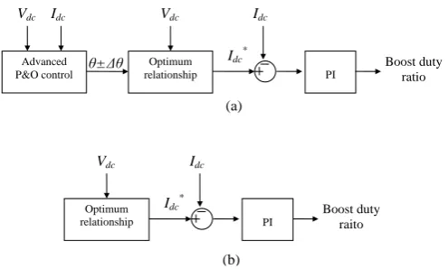
The proposed MPPT technique has two control modes, namely a training mode and a routine mode. The training mode searches for the optimum relationship, given by equation (12). The routine mode is conventional ORB control based on the obtained optimum relationship. The control block diagrams are shown in Fig.4. Only dc voltage and current are measured for MPPT.

Vdc

Advanced P&O control

Idc

Optimum relationship

θ±Δθ

Vdc Idc

Idc*

PI

Boost duty ratio

(a)

Optimum relationship

Vdc Idc

Idc*

PI

Boost duty raito

(b)

Fig. 4 System control block diagrams. (a) Control block diagram for the training mode. (b) Control block diagram for the routine mode.

In the training mode, as shown in Fig. 5, Line A is the optimum relationship which is unknown, and Line B is an arbitrary line initially used. Equation (12) is rewritten as

𝐼𝑑𝑐−𝑜𝑝𝑡 = (𝑎 tan 𝜃)𝑉𝑑𝑐−𝑜𝑝𝑡2 (14)

Considering the values of Vdc2 and Idc are of different orders of magnitude, a in

equation (14) is introduced to match their values. Advanced P&O control is used to search for the optimum relationship by changing the θ value according to the result of the comparison of successive output powers. Observing Figs.3(a) and 5, it can be concluded that, for a given wind speed, the power is always larger when θ is closer to

θopt, and this is demonstrated as the follows.

𝑑𝑃 𝑑𝑉𝑑𝑐|_𝑉

𝑑𝑐=𝑉𝑑𝑐−𝑜𝑝𝑡 = 0

𝑑𝑃 𝑑𝑉𝑑𝑐|_𝑉

𝑑𝑐>𝑉𝑑𝑐−𝑜𝑝𝑡

< 0 (15)

𝑑𝑃 𝑑𝑉𝑑𝑐|_𝑉

𝑑𝑐<𝑉𝑑𝑐−𝑜𝑝𝑡 > 0

Observing Fig.5, at a given wind speed it can be concluded that

𝑑𝑉𝑑𝑐

𝑑𝜃 < 0 (16)

Also applying the chain rule

𝑑𝑃 𝑑𝜃 = 𝑑𝑃 𝑑𝑉𝑑𝑐 𝑑𝑉𝑑𝑐 𝑑𝜃 𝑑𝑃

𝑑𝜃|_{𝜃=𝜃𝑜𝑝𝑡} = 𝑑𝑃 𝑑𝑉𝑑𝑐|_𝑉

𝑑𝑐=𝑉𝑑𝑐−𝑜𝑝𝑡

×𝑑𝑉𝑑𝑐

𝑑𝜃

𝑑𝑃

𝑑𝜃|_{𝜃<𝜃𝑜𝑝𝑡} = 𝑑𝑃 𝑑𝑉𝑑𝑐|_𝑉

𝑑𝑐>𝑉𝑑𝑐−𝑜𝑝𝑡

×𝑑𝑉𝑑𝑐

𝑑𝜃 (17)

𝑑𝑃

𝑑𝜃|_{𝜃>𝜃𝑜𝑝𝑡} = 𝑑𝑃 𝑑𝑉𝑑𝑐|_𝑉

𝑑𝑐<𝑉𝑑𝑐−𝑜𝑝𝑡

×𝑑𝑉𝑑𝑐

𝑑𝜃

Considering equations (15) to (17), it holds that

𝑑𝑃

𝑑𝜃|_{𝜃=𝜃𝑜𝑝𝑡} = 0 𝑑𝑃

𝑑𝜃|_{𝜃<𝜃𝑜𝑝𝑡} > 0 (18)

𝑑𝑃

𝑑𝜃|_{𝜃>𝜃𝑜𝑝𝑡} < 0

Once θopt is obtained, which means the optimum relationship of (14) is known by the

system, the routine mode starts and the system is controlled as by conventional ORB control.

Due to the system elements aging, such as with the wind turbine and generator, any optimum relationship may vary, affecting the wind energy capture efficiency. Online updating can be implemented by running the training mode again after a long period operation.

vw1

vw2

vw3

Vdc2

Idc

Idc=atanθVdc2

θopt

θ

Line B Line A

Region II

Region I

Fig.5 The curves of Idc vs. Vdc2 at different wind speed and the linear equation

A. Training mode

For simplicity, in Fig.5, the area where θ is less than θopt is labelled Region I (the

bottom right part to Line A), and the other area is labelled Region II (the top left part to Line A).

Some important system features should be high lightened to help design the advanced P&O controller.

• Theoretically, θ should always go one direction until it reaches θopt as it is

independent of wind speeds. In other words, if θ is in Region I, then it will always remain in Region I until it reaches θopt.

• The searching speed of the training process is not a main concern as it only operates

once.

1. Initialization

When the wind speed is above the cut-in wind speed, the turbine is started up by using a conventional start-up control method that does not employ an anemometer. Thus before the proposed MPPT is applied, the turbine already has an initial rotor speed.In the initialization block in Fig.6, a and the initial θ in equation (14) are determined. Theoretically, a and the initial θ can be arbitrary values, because an accurate value of

atanθ is obtained via the perturbation of θ. However, for a better performance during the training mode, a method to determine a and initial θ values is suggested.

Since a is used to match the values of Vdc2 and Idc, a simple and effective assignment

method is to use the ratio of rated values of Vdc2 and Idc of a given WECS as the value

of a, which is expressed as

𝑎 = 𝐼𝑑𝑐−𝑟𝑎𝑡𝑒𝑑

𝑉_{𝑑𝑐−𝑟𝑎𝑡𝑒𝑑}2 (19)

For the initial θ value, it is recommended to increase θ gradually to reach θopt rather

than decrease it, because the power increase is much smoother in Region I than in Region II, as shown in Fig.5. Therefore, the initial θ should be a value smaller than

θopt, to guarantee being in Region I. For a mature WECS design, it is safe to assume

that the rated Vdc2 and Idc is close to the MPP at a certain wind speed. Therefore, if a is

Hence the initial θ can be half or one-third of the estimated θopt, or even smaller. Of

course, the determination of a and initial θ can also be obtained by simulation. Note that in the following presentation of the proposed MPPT technique, the initial θ is assumed to be a value smaller than θopt and lies in Region I.

2. Evaluate wind condition

Each time the system starts to change θ, the wind condition should first be evaluated. The system will not change θ unless the wind speed is stable. Thereby the effect of an unstable wind condition during the P&O process can be significantly minimized. As previously mentioned, the training mode only operates once, thus the correct perturbation is much more important than the search speed.

A simple method is to continue evaluating the difference of successive samples of output power, ΔPout. Defining an index, steady_mark, as

steady_mark =Δ𝑃𝑜𝑢𝑡

𝑃𝑜𝑢𝑡 (20)

If the steady_mark is smaller than a threshold, then it can be assumed that the wind speed is stable and the P&O process can start.

3. Determining the sign of Δθ

With a change of Δθ, the corresponding change of power, ΔP, is measured. If a previous positive Δθ results in an output power increase, then it means θ is still in Region I. Hence the next Δθ should still be positive, and vice versa. Such a basic P&O control can assure the θ goes in the right direction with a stable wind speed and gradually approaches θopt. However, if there is a sudden drop of wind speed right after

process into making a wrong decision. Such a condition slows down the search for the optimum relationship. Advanced P&O control is employed to minimize the influence.

As mentioned, theoretically, if the initial θ is in Region I, it should keep increasing until it reaches θopt. This process is independent of wind speed. Therefore the signs of

previous Δθ can help judge the current sign. It is logical to assume that if most of the previous Δθ are positive, which means θ is in Region I, then it is highly probable that it is still in Region I even though the change of power shows that it may now be in Region II.

To achieve such a concept, the previous signs of Δθ are recorded in an array sign[n] (n>0), where n is the number of previous Δθ. If a previous Δθ is in Region I, then its

sign is labelled as +1, otherwise it is labelled as -1, as shown in (21).

𝑠𝑖𝑔𝑛[𝑛] = {+1 (In Region I)

−1 (In Region II) 𝑛 > 0 (21)

According to the comparison of successive output power, the present sign[0] is also judged and obtained, where 0 means it is the current sign. Labelled in the same way, as shown in (22)

𝑠𝑖𝑔𝑛[0] = {+1 (In Region I)

−1 (In Region II) (22)

The sum of the sign [n] (n0)

𝑅 = ∑𝑛_𝑘=0𝑠𝑖𝑔𝑛[𝑘] (23)

If R>0, more than half of the previous Δθ are positive, then it is highly possible that the current θ still lies in Region I, and the next Δθ should be positive. Otherwise, if

𝑠𝑖𝑔𝑛[𝑛] = 𝑠𝑖𝑔𝑛[𝑛 − 1]

  

(24)

𝑠𝑖𝑔𝑛[1] = 𝑠𝑖𝑔𝑛[0]

Using such a method, unless the θ lies in Region II, otherwise, a sudden wind change does not affect R, and θ will keep changing in correct direction. And if θ lies in Region II, then more and more negative sign[n] appears and finally R<0. Therefore, this method can effectively minimize the influence of wind speed change.

The value of n represents the ability of resistance to the successive wind speed drops. For example, if n=2, then two successive wind speed drops may cause an incorrect θ change direction, and if n=4, then three successive wind speed drops may cause misjudgement. However, with the increase of n, the system response slows down as it needs more steps to confirm which region θ really lies in. Therefore the value of n is a trade-off of search accuracy and speed. Considering that θ only varies when the wind speed is stable, such successive sudden wind speed drop situation is rare. Thus n can be a small value, i.e. 4 or 6. It should be noted that n must be an even number, so the

sum of the sign[n](n0) never equals to zero. The combination of the control strategy in Section IV-A-2 and Section IV-A-3 makes the P&O process robust and accurate in actual fluctuating wind conditions.

4. Determining the amplitude of θ

The amplitude of Δθ is then determined as shown in Fig.6. When θ is around θopt, it

the oscillation range will also be reduced, and finally θ converges to θopt. Once the

optimum relationship is obtained, the training mode ends and routine mode starts. An array amplitude[m] (m>0) is introduced to control the amplitude of Δθ. Similar to

sign[n], it is related to previous mΔθ, and labelled in a similar way.

𝑎𝑚𝑝𝑙𝑖𝑡𝑢𝑑𝑒[𝑚] = {+1 (In Region I)

−1 (In Region II) 𝑚 > 0 (25)

Every time a change of θ occurs, the array amplitude[m] is updated as follows,

𝑎𝑚𝑝𝑙𝑖𝑡𝑢𝑑𝑒[𝑚] = 𝑎𝑚𝑝𝑙𝑖𝑡𝑢𝑑𝑒[𝑚 − 1]

  

(26)

𝑎𝑚𝑝𝑙𝑖𝑡𝑢𝑑𝑒[1] = 𝑎𝑚𝑝𝑙𝑖𝑡𝑢𝑑𝑒[0]

And the amplitude[0]=+1, if the system confirms that the current θ still lies in Region I, or amplitude[0]=-1, if lying in Region II.

The amplitude of Δθ is expressed as

|Δ𝜃| =∑𝑚𝑘=1𝑎𝑚𝑝𝑙𝑖𝑡𝑢𝑑𝑒[𝑘]

𝑚 𝜃𝑓

0 ≤ ∑𝑚𝑘=1𝑎𝑚𝑝𝑙𝑖𝑡𝑢𝑑𝑒[𝑘]

𝑚 ≤ 1 (27)

where θf is the fundamental amplitude value. Initially, amplitude[k]=+1 (k=0,1,2,…,m)

and ∑𝑚_𝑘=1𝑎𝑚𝑝𝑙𝑖𝑡𝑢𝑑𝑒[𝑘]= 𝑚. Therefore |Δθ|= θf, and θ approaches θopt with a

relatively large amplitude. Once θ is larger than θoptand lies in Region II, the value of

∑𝑚_𝑘=1𝑎𝑚𝑝𝑙𝑖𝑡𝑢𝑑𝑒[𝑘] begins to decrease, leading to a smaller amplitude. When θ

oscillates around θopt, Δθ becomes smaller and smaller, with the number of -1 being

The value of m relates to the reducing rate of the Δθ amplitude. m should be large enough, so that the Δθ amplitude will reduce gradually. The critical control parameters, a, initial θ, steady_mark, n, m and θf discussed in this section should be

obtained via simulation to get the optimum performance. A flow chart of the proposed technique is shown in Fig.6.

B. Routine mode & online updating

When the training mode ends, the optimum relationship of equation (14) is obtained. The system starts routine mode, tracks MPP using conventional ORB control.

Moreover, due to system element aging and system parameter change, the obtained relationship may be no longer optimum. Online updating can be implemented by running the training mode again to search for the new optimum relationship.

C. Comparison with conventional MPPT methods

Table 1 Comparison with traditional MPPT methods Anemometer System

pre-knowledge

Tracking speed

Oscillation at MPP

Online updating

TSR Yes Required Fast No No

P&O No Not required Slow Yes Yes

ORB No Required Fast No No

Proposed technique

Initialization

Start P&O Process

Evaluate wind condtion

Change θ

θ±Δθ

Compare successive output powers

Determine the amplitude of Δθ

Stable wind condition

Unstable wind condition

Switch to routine mode

|Δθ|>Threshold

Routine mode

|Δθ|<Threshold

Training mode

Determine the sign of Δθ

V. Simulation results

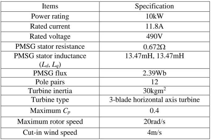
MATLAB/Simulink simulations can verify the performance of the proposed MPPT technique. The WECS scheme is similar to that shown in Fig.2. The parameters of PMSG and wind turbine are summarized in Table 2, while the control parameters are summarized in Table 3.

Table 2 PMSG and wind turbine parameters in simulation

Items Specification

Power rating 10kW

Rated current 11.8A

Rated voltage 490V

PMSG stator resistance 0.672 PMSG stator inductance

(Ld, Lq)

13.47mH,13.47mH

PMSG flux 2.39Wb

Pole pairs 12

Turbine inertia 30kgm2

Turbine type 3-blade horizontal axis turbine

Maximum Cp 0.4

Maximum rotor speed 20rad/s

Cut-in wind speed 4m/s

Table 3 Control parameters in simulation

Parameters Values

a in (12) 4e-5

Initial θ 10°

n in (22) 4

m in (26) 50

θf in (28) 2°

Δθ Threshold 0.4°

Simulation results are shown in Fig.7. At time 0 second, it is assumed that the wind turbine start-up period is over and the turbine already has an initial rotor speed. Before t4, the system is in the training mode, where Figs.7(c)(d) show that θ increases

condition, as show in Fig.7(a). Fig.7(e) shows the rotor speed. The training mode takes less than 50 seconds, and then the system starts the routine mode once θopt

settles. Win d speed (m /s) t4 (a) Time (s) Outp u t po wer (W) t4

t1 t2 t3 Time (s) (b)

t4

t1 t2 t3 Time (s) (c)

Cp

t4

t1 t2 t3 Time (s) (d)

θ

(°)

t4

t1 t2 t3 Time (s) (e)

Ro tor sp eed (ra d /s )

Fig.7 Simulation results of the proposed MPPT technique. (a) wind speed. (b) output power. (c) power coefficient. (d) angle, θ. (e) rotor speed.

Between t1 and t2, the wind speed is unstable and reduces gradually as shown in

Fig.7(a). In such an unstable wind condition, the controller in Section IV-A-2 guarantees that the P&O process does not operate. Fig.8 shows the details of the t1 to

t2 period. In Fig.8(a), the wind speed gradually decrease from 12m/s to 10m/s, and the

operational, the power efficiency, Cp, having been achieved does not decrease, as

shown in Fig.8(c).

Win

d

speed

(m

/s)

t1 Time (s) (a) t2

Outp

u

t po

wer

(W)

t1 Time (s) (b) t2

Cp

t1 Time (s) (c) t2

θ

(°)

t1 Time (s) (d) t2

Ro

tor

sp

eed

(ra

d

/s

)

t1 Time (s) (e) t2

Fig.8 The detail simulation results of t1-t2 period. (a) wind speed. (b) output power. (c)

power cofficient. (d) angle, θ. (e) rotor speed.

During t2 to t3 shown in Fig.7, there is a sudden wind speed drop immediately after

the θ adjustment. The details are shown in Fig.9. Fig.9(d) shows that at ta, θ increases

a Δθ value, but suddenly at tb the wind speed drops from 10m/s to 9m/s. In Fig.9(b),

Win

d

speed

(m

/s)

(a) t3

t2 ta tb Time (s) tc

Outp

u

t po

wer

(W)

(b) _t3

t2 ta tb Time (s) tc

Cp

(c) t3

t2 ta tb Time (s) tc

θ

(°)

(d) t3

t2 ta tb Time (s) tc

Ro

tor

sp

eed

(ra

d

/s

)

(e) _t3

t2 ta tb Time (s) tc

Fig.9 The detail simulation results of t2-t3 period. (a) wind speed. (b) output power. (c)

power coefficient. (d) angle, θ. (e) rotor speed.

Between t3 and t4 shown in Fig.7, θ is close to θopt, and it starts to oscillate. The details

are shown in Fig.10. From t3 to t4, θ oscillates with gradually reducing amplitude.

Meanwhile, the total oscillating band decreases, which is shown in Fig.10(d) between 25s and 50s. Although θ is oscillating, the power and Cp is relatively stable as shown

in Fig.10(a) and (c). This is due to the aforementioned flat-topped Cp curve. The rotor

Win

d

speed

(m

/s)

t3 Time (s) (a) t4

Outp

u

t po

wer

(W)

t3 Time (s) (b) t4

Cp

t3 Time (s) (c) t4

θ

(°)

t3 Time (s) (d) t4

Ro

tor

sp

eed

(ra

d

/s

)

t3 Time (s) (e) t4

Fig.10 The detail simulation results of t3-t4 period. (a) wind speed. (b) output power.

(c) power efficiency. (d) angle, θ. (e) rotor speed.

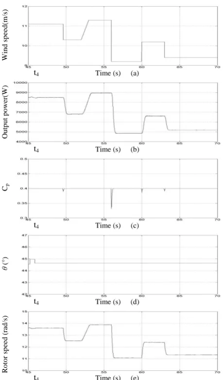
At t4, θ finally converges to the optimum value as shown in Fig.7. The total time

required for the training mode of the 10kW system is less than 50s. Moreover, it also shows that Cpapproaches close to the maximum value in about 15s. This proves that

the advance P&O process can obtain the optimum relationship in a short time. After t4,

Win

d

speed

(m

/s)

t4 Time (s) (a)

Outp

u

t po

wer

(W)

t4 Time (s) (b)

Cp

t4 Time (s) (c)

θ

(°)

t4 Time (s) (d)

Ro

tor

sp

eed

(ra

d

/s

)

t4 Time (s) (e)

Fig. 11 The detail simulation results of routine mode after t4. (a) wind speed. (b)

output power. (c) power efficiency. (d) angle, θ.(e) rotor speed.

VI. Experimental results

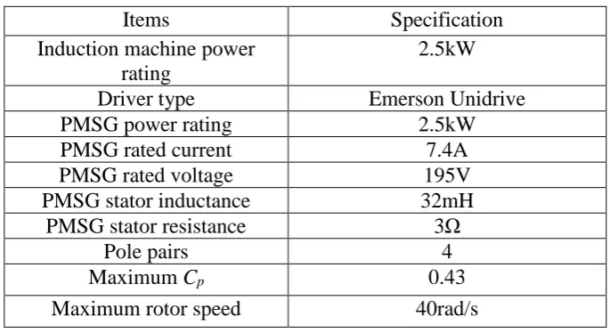
point. The boost output voltage is maintained constant by a switch to model a constant voltage DC link. The system parameters are summarized in Table 4, and the control parameters are summarized in Table 5.

Table 4 Experimental system parameters

Items Specification

Induction machine power rating

2.5kW Driver type Emerson Unidrive

PMSG power rating 2.5kW

PMSG rated current 7.4A

PMSG rated voltage 195V

PMSG stator inductance 32mH

PMSG stator resistance 3Ω

Pole pairs 4

Maximum Cp 0.43

Maximum rotor speed 40rad/s

Table 5 Practical control parameters

Parameters Values

a in (12) 2e-4

Initial θ 5°

n in (22) 4

m in (26) 50

θf in (28) 1°

Δθ Threshold 0.2°

fast response and good performance. The results confirm the validity of the proposed MPPT technique. ` DSP Tri-Core 1796B Host PC

Boost converter and load

Machine Driver DSP Tri-Core 1796B ` Host PC

Fig.12 The wind energy conversion system test rig

Time (s) (a)

Win

d

speed

(m

/s)

Time (s) (b)

Outp u t po wer ( W )

Time (s) (c)

Cp

Time (s) (d)

θ

(°)

(m/s)

Time (s) (e)

Ro tor sp eed ( ra d /s ) (m/s)

VII. Discussion

The proposed MPPT technique is presented and simulated for the WECS shown in Fig. 2. However, this technique is a general method that can be applied to different topologies as long as the system satisfies equation (12). The power rating may be able to be extended to MW level. As the proposed MPPT technique searches for an optimum relationship rather than specific points, the system is controlled smoothly.

The concept of searching for an optimum relationship can be extended to the systems control based on optimum relationships such as T=k1Ω2 [26], or P=k2Ω3 [19], where T

is the electrical torque. As discussed, equation (12) is based on the assumption that the terminal voltage varies linearly with the turbine rotor speed, therefore the Cpachieved

may not be optimum for all wind speeds. However, when using the optimum relationship of T=k1Ω2 and P=k2Ω3 to control the system, the Cp achieved may be

nearer to optimum.

VIII. Conclusion

Reference

[1] U.S. Energy Information Administration (EIA) Report #: DOE/EIA-0484(2010), 2010.

[2] J. F. Manwell, J. G. McGowan, and A. L. Rogers, Wind Energy Explained. New York: Wiley, 2002, p. 88.

[3] Q. Wang, and L.-C. Chang, “An intelligent maximum power extraction algorithm for inverter-based variable speed wind turbine systems,” IEEE Trans. Power Electron., vol. 19, no. 5, pp. 1242-1249, Sep. 2004.

[4] I. K. Buehring, and L. L. Freris, “Control policies for wind energy conversion systems,” Proc. Inst. Elect. Eng. C, vol. 128, pp. 253–261, Sept. 1981.

[5] T.Thiringer, and J.Linders, “Control by variable rotor speed of a fixed-pitch wind turbine operating in a wide speed range,” IEEE Trans. Energy Convers., vol. 8, no. 3, pp. 520–526, Sep. 1993.

[6] R. M. Hilloowala, and A. M. Sharaf, “A rule-based fuzzy logic controller for a PWM inverter in a stand alone wind energy conversion scheme,” IEEE Trans. Ind.

Appl., vol. 31, no. 1, pp. 57–65, Jan./Feb. 1996.

[7] R. Chedid, F. Mrad, and M. Basma, “Intelligent control of class of wind energy conversion systems,” IEEE Trans. Energy Convers., vol. 14,pp. 1597–1604, Dec.

1999.

[8] K. Johnson, L. Fingersh, M. Balas, and L. Pao, “Methods for increasing region 2 power capture on a variable speed wind turbine,” J. Solar EnergyEng., vol. 126, no. 4, pp. 1092–1100, 2004.

[10] M. Ermis, H. B. Ertan, E. Akpinar, and F. Ulgut, “Autonomous wind energy conversion system with a simple controller for maximum-power transfer,” IEE Proc. B, Electr. Power Appl., 1992, 139, (5),pp. 421–428.

[11] R. Datta and V. T. Ranganathan, “A method of tracking the peak power points for a variable speed wind energy conversion system,” IEEE Trans. Energy Convers.,

vol. 18, no. 1, pp. 163–168, Mar. 1999.

[12] M. G. Simoes, B. K. Bose, and R. J. Spiegel, “Fuzzy logic based intelligent control of a variable speed cage machine wind generation system,” IEEE Trans.

Power Electron., vol. 12, pp. 87–95, Jan. 1997.

[13] M. G. Simoes, and B. K. Bose, “Design and performance evaluation of fuzzy-logic-based variable-speed wind generation system,” IEEE Trans. Ind. Appl., vol. 33, no. 4, pp. 956–965, Jul./Aug. 1997.

[14] E. Koutroulis, and K. Kalaitzakis, “Design of a maximum power tracking system for wind-energy-conversion applications,” IEEE Trans. Ind. Electron., vol. 53, no. 2, pp. 486–494, Apr. 2006.

[15] M. R. Kazmi, H. Goto, H. Guo, and O. Ichinoku ra, “A Novel Algorithm for Fast and Efficient Speed-Sensorless Maximum Power Point Tracking in Wind Energy Conversion Systems,” IEEE Trans. Ind. Electro., to be published.

[16] S. Bhowmik, R. Spée, and J. H. R. Enslin, “Performance optimization for doubly fed wind power generation systems,” IEEE Trans. Ind. Applicat., vol. 35, pp. 949–958,

July/Aug. 1999.

[18] A. Neris, N. Vovos, and G. Giannakopaulos, “A variable speed wind energy conversion scheme for connection to weak ac systems,” IEEE Trans. Energy Convers.,

vol. 14, no. 1, pp. 122–127, Mar. 1999.

[19] W. Lu and B. T. Ooi, “Optimal acquisition and aggregation of offshore wind power by multiterminal voltage-source HVDC,” IEEE Trans. Power Del., vol. 18, no. 1, pp. 201–206, Jan. 2003.

[20] E. Muljadi and C. P. Butterfield, “Pitch-controlled variable-speed wind turbine generation,” IEEE Trans. Ind. Applicat., vol. 37, pp. 240–246,Jan./Feb. 2001.

[21] B. Shen, B. Mwinyiwiwa, Y. Zhang, and B.-T. Ooi, “Sensorless maximum power point tracking of wind by DFIG using rotor position phase lock loop (PLL),”

IEEE Trans. Power Electron., vol. 24, pp. 942–951, Apr.2009.

[22] M. Chinchilla, S. Arnaltes, and J. C. Burgos, “Control of permanent-magnet generators applied to variable-speed wind-energy systems connected to the grid,”

IEEE Trans. Energy Conv., vol. 21,no. 1, pp. 130–135, Mar. 2006.

[23] A. Mirecki, X. Roboam, and F. Richardeau, “Architecture complexity and energy efficiency of small wind turbines,” IEEE Trans. Ind. Electron., vol. 54, no. 1, pp. 660–670, Feb. 2007.

[24] K. Tan and S. Islam, “Optimum control strategies in energy conversion of PMSG wind turbine system without mechanical sensors,” IEEE Trans. Energy Convers., vol.

19, no. 2, pp. 392–399, Jun. 2004.

[25] S. Morimoto, H. Nakayama, M. Sanada, and Y. Takeda, “Sensorless output maximization control for variable-speed wind generation system using IPMSG,”

IEEE Trans. Ind. Appl., vol. 41, no. 1, pp. 60–67,Jan./Feb. 2005.

generation,” Proc. Inst. Elect. Eng., Electr. PowerAppl., vol. 143, no. 3, pp. 231–241,

May 1996.

[27] C.-T. Pan and Y.-L. Juan, “A novel sensorless MPPT controller for a high-efficiency microscale wind power generation system,” IEEE Trans. Energy

Conversion, to be published.

[28] M. E. Haque, M. Negnevitsky, and K. M. Muttaqi, "A Novel Control Strategy for a Variable-Speed Wind Turbine with a Permanent-Magnet Synchronous Generator,"

IEEE Trans. Industry Applications, vol. 46, no. 1, pp. 331-339, Jan.-Feb. 2010.

[29] Z. Chen, and E. Spooner, “Grid power quality with variable-speed wind turbines,”

IEEE Trans. Energy Conv., vol. 16, no. 2, pp. 148–154, June 2001.

[30] S.-H. Song, S.-I. Kang, and N.-K. Hahm, “Implementation and control of grid connected ac–dc–ac power converter for variable speed wind energy conversion system,” in Proc. IEEE APEC, vol. 1, pp. 154–158, 2003.

[31] H.-B. Zhang, J. Fletcher, N. Greeves, S. J. Finney, and B. W. Williams, “One-power-point operation for variable speed wind/tidal stream turbines with synchronous generators”, IET Renewable Power Generation, vol. 5, no. 1, pp. 99-108, Jan. 2011.

[32] H. Li, K. L. Shi, and P. G. McLaren, “Neural-network-based sensorless maximum wind energy capture with compensated power coefficient,” IEEE Tran. Ind.

Appl., vol. 41, no. 6, pp. 1548–1556, Nov./Dec. 2005.

[34] J. A. Baroudi, V. Dinavahi, and A. M. Knight, “A review of power converter topologies for wind generators,” Renew. Energy, vol. 32, no. 14, pp. 2369–2385, Nov.

2007.

[35] O. Anaya-Lara, N. Jenkins, J. Ekanayake, P. Cartwright, and M. Hughes, Wind Energy Generation: Modelling and Control. New York: Wiley,Sep. 2009.

[36] A. E. Fitzgerald, C. Kingsley, and S. D. Umans, Electric Machinery, Fifth ed: McGraw-Hill Book Company, 1992.

[37] M. H. Rashid, Power Electronics Circuits, Devices, and Applications. Englewood Cliffs, NJ: Prentice-Hall, 1993.

[38] T. F. Chan and L. L. Lai, “An axial-flux permanent-magnet synchronous generator for a direct-coupled wind turbine system,” IEEE Trans. Energy Convers.,

vol. 22, no. 1, pp. 86–94, Mar. 2007.

[39] C. Liu, K. T. Chau, J. Z. Jiang, and L. Jian, “Design of a new outer-rotor permanent magnet hybrid machine for wind power generation,” IEEE Trans. Magn.,

vol. 44, no. 6, pp. 1494–1497, Jun. 2008.

[40] G. D. Moor and H. J. Beukes, “Maximum power point trackers for wind turbines,” in Proc. 35th Annu. IEEE Power Electron. Spec. Conf., Aachen,Germany, Jun. 2004, pp. 2044–2049.

[41] A. Tapia, G. Tapia, J. Ostolaza, and J. Saenz, “Modeling and control of a wind turbine driven doubly fed induction generator,” IEEE Trans. Energy Convers., vol. 18,

no. 2, pp. 194–204, Jun. 2003.