This is a repository copy of
Unspanned macroeconomic factors in the yield curve
.
White Rose Research Online URL for this paper:
http://eprints.whiterose.ac.uk/75107/
Version: Published Version
Monograph:
Coroneo, Laura orcid.org/0000-0001-5740-9315, Giannone, Domenico and Modugno,
Michele (2014) Unspanned macroeconomic factors in the yield curve. Working Paper.
Finance and Economics Discussion Series . Federal Reserve Board, Washington, D.C. ,
Brussels.
eprints@whiterose.ac.uk Reuse
Items deposited in White Rose Research Online are protected by copyright, with all rights reserved unless indicated otherwise. They may be downloaded and/or printed for private study, or other acts as permitted by national copyright laws. The publisher or other rights holders may allow further reproduction and re-use of the full text version. This is indicated by the licence information on the White Rose Research Online record for the item.
Takedown
If you consider content in White Rose Research Online to be in breach of UK law, please notify us by
Finance and Economics Discussion Series
Divisions of Research & Statistics and Monetary Affairs
Federal Reserve Board, Washington, D.C.
Unspanned macroeconomic factors in the yield curve
Laura Coroneo, Domenico Giannone, and Michele Modugno
2014-57
Unspanned macroeconomic factors in the yield curve
Laura Coroneo University of York
Domenico Giannone
Luiss University of Rome, ECARES, EIEF and CEPR
Michele Modugno
Board of Governors of the Federal Reserve System
July 30, 2014
Abstract
In this paper, we extract common factors from a cross-section of U.S. macro-variables and Trea-sury zero-coupon yields. We find that two macroeconomic factors have an important predictive content for government bond yields and excess returns. These factors are not spanned by the cross-section of yields and are well proxied by economic growth and real interest rates.
JEL classification codes: C33, C53, E43, E44, G12.
Keywords: Yield Curve; Government Bonds; Factor models; Forecasting.
1
Introduction
Government bond yields with different maturities and macroeconomic variables are both
character-ized by a high degree of comovement, indicating that the bulk of their dynamics is driven by a few
common forces. Three common factors, usually interpreted as the level, slope and curvature of the
yield curve, can explain changes and shifts of the entire cross-section of yields, see Litterman and
Scheinkman (1991). Although there is less consensus on the number and nature of macroeconomic
factors, two factors, one nominal and one real, summarize well the dynamics of a large variety of
macroeconomic indicators for the United States, see Sargent and Sims (1977), Giannone, Reichlin
and Sala (2005) and Watson (2005).
Macroeconomic factors and yield curve factors are also characterized by a strong interaction.
The short end of the yield curve moves closely to the policy instrument under the direct control
of the central bank, which responds to changes in inflation, economic activity, or other economic
conditions, see Taylor (1993). The average level of the yield curve is usually associated with the
inflation rate and the spread between long and short rates with temporary business cycles
condi-tions, see Diebold, Rudebusch and Aruoba (2006). For these reasons, macroeconomic information
have been shown to help forecasting future interest rates and excess bond returns, see Ang and
Piazzesi (2003), M¨onch (2008), De Pooter, Ravazzolo and van Dijk (2007), Favero, Niu and Sala
(2012) and Ludvigson and Ng (2009).
In this paper, we aim at identifying the factors summarizing macroeconomic information that is
not spanned by the traditional yield curve factors. The economic literature so far has not addressed
this problem since in existing studies macroeconomic factors are either proxied by preselected
observable variables, see Bianchi, Mumtaz and Surico (2009), Dewachter and Lyrio (2006), Diebold
et al. (2006), Joslin, Priebsch and Singleton (2014) and Wright (2011), or extracted from a large
set of macroeconomic indicators and treated separately from the yield curve factors, see Ang and
Piazzesi (2003), Favero et al. (2012), Ludvigson and Ng (2009), M¨onch (2008) and M¨onch (2012).
com-ponents that we extract simultaneously with the traditional yield curve factors. The latter are
identified by constraining the loadings to follow the smooth pattern proposed by Nelson and Siegel
(1987). More specifically, our empirical model is a Dynamic Factor Model (DFM) for Treasury
zero-coupon yields and a representative set of macroeconomic variables with restrictions on the
factor loadings. Estimation is performed using a Quasi-Maximum Likelihood approach, as
pro-posed by Doz, Giannone and Reichlin (2012). This procedure is easily implementable using the
Kalman smoother and the Expectation Maximization algorithm. The estimator has been shown
to be feasible when the number of variables is large, and robust to non Gaussianity and to the
presence of weak cross-sectional correlation among the idiosyncratic terms. We validate the model
by assessing the forecasting ability for yields and excess returns of US government bonds.
Using monthly U.S. data from January 1970 to December 2008, we find that a significant
component of macroeconomic information is not captured by the yield curve factors and, at the
same time, is unspanned by the yield curve, in the sense that it does not affect contemporaneously
the cross-section of yields. The unspanned macroeconomic information is driven by two factors
that are well proxied by economic growth and real interest rates. These factors have substantial
predictive information for bond yields and excess bond returns, in spite of the fact that they do
not affect contemporaneously the shape of the yield curve. The macro-yields model explains up
to 55% of the variation in excess bond returns and outperforms all existing models in forecasting
bond yields and excess returns.
The paper is organized as follows. Section 2 presents the macro-yields model. Section 3 describes
the data, the estimation procedure and the information criteria used for model selection. Section
4 describes the empirical results and in-sample validation of the model. Section 5 reports out of
2
The macro-yields model
The macro-yields model that we propose is a dynamic factor model for the joint behavior of
gov-ernment bond yields and macroeconomic indicators. The cross-section of yields is described by the
traditional level, slope and curvature factors. Macroeconomic variables load on both the yield curve
factors as well as on some additional macro factors, that capture the information in macroeconomic
variables over and above the yield curve factors. In addition, these additional macro factors are
assumed to not provide any information about the contemporaneous shape of the yield curve. In
practice, the level, slope and curvature implied by the Nelson and Siegel (1987) model are assumed
to be spanned by both the bond yields and macroeconomic variables. The additional macro
fac-tors, instead, are contemporaneously loaded only by the macroeconomic variables and, thus, are
unspanned by the cross-section of yield. The joint dynamics of the factors is an unrestricted vector
autoregression and the idiosyncratic components follow independent univariate autoregressions. In
what follows we detail on each of the points.
More specifically, we assume that yields on bonds with different maturities are driven by three
common factors. Denoting byyt theNy×1 vector of yields with Ny different maturities at timet, we have
yt = ay+ Γyy Fty+vty, (1)
where Fty is a 3×1 vector containing the latent yield-curve factors at time t, Γyy is a Ny ×3 matrix of factor loadings, andvyt is anNy×1 vector of idiosyncratic components. The yield curve factorsFty are identified by constraining the factor loadings to follow the smooth pattern proposed by Nelson and Siegel (1987) (hereafter NS)
ay = 0; Γ(yyτ)=
1 1−e
−λτ λτ
1−e−λτ λτ −e
−λτ
≡Γ(N Sτ), (2)
functional form of the factor loadings, implies that the three yield curve factors can be interpreted
as the level, slope and curvature of the yield curve. Indeed, the loading equal to one on the first
factor, for all maturities, implies that an increase in this factor increases all yields equally, shifting
the level of the yield curve. The loadings on the second factor are large for short maturities,
decaying to zero for the long ones. Accordingly, an increase in the second factor increases the slope
of the yield curve. Loadings on the third factor are zero for the shortest and the longest maturities,
reaching the maximum for medium maturities. Therefore, an increase in this factor augments the
curvature of the yield curve. The specific shape of the loadings depends on the decay parameterλ,
which we calibrate to the value that maximizes the loading on the curvature factor for the yields
with maturity 30 months, as in Diebold and Li (2006).
Given these particular functional forms for the loadings on the three yield curve factors, one
can summarize movements in the term structure of interest rates into three factors which have a
clear-cut interpretation. The NS factors are just linear combinations of yields. The level factor can
be proxied by the long term yield, the slope by the spread between the long and short maturity yield
(first derivative) and the curvature by sum of the spreads between a medium and a long term yield,
and between a medium and the short term yield (second derivative), see Diebold and Li (2006).1
Due to its flexibility and parsimony, the NS model accurately fits the yield curve and performs
well in out-of-sample forecasting exercises, as shown by Diebold and Li (2006) and De Pooter et al.
(2007). For these reasons, fixed-income wealth managers in public organizations, investment banks
and central banks rely heavily on NS type of models to fit and forecast yield curves, see BIS (2005),
ECB (2008), G¨urkaynak, Sack and Wright (2007) and Coroneo, Nyholm and Vidova-Koleva (2011).
Macroeconomic variables, are assumed to be potentially driven by two sources of co-movement,
the yield curve factorsFty and macro specific factors. Denoting byxttheNx×1 vector of macroe-conomic variables at time t, we have
xt = ax+ Γxy Fty+ Γxx Ftx+vtx, (3)
where Ftx is an r ×1 vector of macroeconomic latent factors, Γxy is a Nx×3 matrix of factor loadings on the yield curve factors, Γxx is a Nx×r matrix of factor loadings on the macro factors, and vxt is an Nx×1 vector of idiosyncratic components.
The yield curve and the macroeconomic factors are extracted by estimating (1) and (3)
simul-taneously yt xt = 0 ax +
Γyy Γyx Γxy Γxx
Fty Ftx
+
vyt vtx
, Γyy = ΓN S, Γyx= 0, (4)
where ΓN S is defined according to (2).
The joint dynamics of the yield curve and the macroeconomic factors follow a VAR(1)
Fty Ftx
= µy µx +
Ayy Ayx Axy Axx
Fty−1 Ftx−1
+
uyt uxt
,
uyt uxt
∼N
0,
Qyy Qyx Qxy Qxx
. (5)
The idiosyncratic components collected in vt = [vty vxt]′ are modelled to follow independent autoregressive processes
vt=Bvt−1+ξt, ξt∼N(0, R) (6)
whereB and Rare diagonal matrices, implying that the common factors fully account for the joint
correlation of the observations. The residuals to the idiosyncratic components of the individual
variables, ξt, and the innovations driving the common factors, ut, are assumed to be normally distributed and mutually independent. This assumptions implies that the common factors are not
allowed to react to variable specific shocks.
The assumptions of Gaussianity and of independence among idiosyncratic components might
be sources of miss-specification. It is hard to relax these restrictions since they are necessary
to retain parsimony, insure identification of the common and idiosyncratic components and limit
computational complexity. However, Doz et al. (2012) have shown that, if the factor structure is
presence of limited correlations among idiosyncratic components.
Allowing Γxy to be different from zero is crucial to insure that the macroeconomic factors Ftx capture only those source of co-movement in the macroeconomic variables that are not already
spanned by the yield curve factors. Existing studies, instead, have imposed a block-diagonal
struc-ture of the factor loadings (Γxy = 0 and Γyx = 0), either explicitly, as in M¨onch (2012),2 either implicitly by extracting the macro factors exclusively from macroeconomic variables, as in
Ludvig-son and Ng (2009).
Assuming that macroeconomic factors do not provide any information about the
contemporane-ous shape of the yield curve (Γyx= 0) restricts the macroeconomic factorsFtx to be unspanned not only by the yield factors but also by the entire cross-section of yields. This restriction is expected
to be immaterial since, as stressed above, the yield factors Fty are notoriously effective at fitting the entire yield curve.
In this remainder of the paper we will maintain the restriction Γyx = 0 and leave Γxy un-restricted, unless otherwise mentioned. The block-diagonal model (Γxy = 0, Γyx = 0) and the unrestricted model (Γxy 6= 0) are considered in Appendix D.
3
Estimation and preliminary results
3.1 Data
We use monthly U.S. Treasury zero-coupon yield curve data spanning the period January 1970
to December 2008. The bond yield data are taken from the Fama-Bliss dataset available from
the Center for Research in Securities Prices (CRSP) and contain observations on three months
and one through five-year zero coupon bond yields. The macroeconomic dataset consists of 14
macroeconomic variables, which include five inflation measures, seven real variables, the federal
funds rate and a money indicator. Appendix B contains a complete list of the macroeconomic
2M¨onch (2012) estimates his model with Bayesian methods since he claims that “Estimation of the model via
variables along with the transformation applied to ensure stationarity. Following Ang and Piazzesi
(2003), De Pooter et al. (2007), Diebold et al. (2006) and M¨onch (2008), we use annual growth
rates for all variables, except for capacity utilization, the federal funds rate, the unemployment rate
and the manufacturing index which we keep in levels.3
3.2 Estimation
Equations (4)–(6) describe a restricted state-space model with autocorrelated idiosyncratic
compo-nents for which maximum likelihood estimators of the parameters are not available in closed form.
Conditionally on the factors, the model reduces in a set of linear regressions. As consequence, the
Maximum Likelihood estimates can be easily computed using the Expectation Maximization (EM)
algorithm, as described in detail in Appendix A.4
We initialize the yield curve factors with the NS factors using the two-steps OLS procedure
introduced by Diebold and Li (2006). We then project the macroeconomic variables on the NS
factors and use the principal components of the residuals of this regression to initialize the
un-spanned macroeconomic factors. Γyy is restricted to be equal to the NS loadings. All the other parameters are initialized with the OLS estimates obtained using the initial guesses of yield and
macro factors described above. Given the initial parameters, a new set of factors is obtained using
the Kalman smoother. If we stop at this stage, we have the two-step procedure of Doz, Giannone
and Reichlin (2011). Roughly speaking, Maximum Likelihood estimates are obtained by iterating
these two steps until convergence, see Doz et al. (2012).5
For comparison, we also estimate an only-yields model, which uses only the information
con-tained in the yields. This is a restricted version of the macro-yields model in equations (4)–(6) with
3Since the selection of variables has an element of arbitrariness, we have performed robustness checks with an
alternative databases constructed by Banbura, Giannone, Modugno and Reichlin (2012) that includes all the variables that are constantly monitored by market participants. Results, reported in a separate Appendix, show that the main findings are confirmed.
4Using the Expectation Conditional Restricted Maximization (ECRM) algorithm is also possible to estimateλ, but, despite the increase in the computation burden, the empirical results remain qualitatively similar to those obtained by setting λ to the value that maximizes the loading of the the yields with maturity 30 months on the curvature factor.
5In Appendix E, we compare the initial estimates and find that the Maximum Likelihood provide significant
Qyx=Ayx = Γxy = 0 and can hence be estimated using the same procedure.
3.3 Model selection
The macro-yields model decomposes variations in yields and macroeconomic variables into yield
curve factors, unspanned macroeconomic factors and idiosyncratic noises. The yield curve factors
are identified as the NS factors which have a clear interpretation as level, slope and curvature.
However, the true number of unspanned macroeconomic factors is unknown. We select the optimal
number of factors using an information criteria approach. The idea is to choose the number of
factors that maximizes the general fit of the model using a penalty function to account for the loss
in parsimony.
Bai and Ng (2002) derive information criteria to determine the number of factors in approximate
factor models when the factors are estimated by principal components. They also show that their
IC3information criterion can be applied to any consistent estimator of the factors provided that the
penalty function is derived from the correct convergence rate. For the quasi-maximum likelihood
estimator, Doz et al. (2012) show that it converges to the true value at a rate equal to
CN T∗2 = min √
T , N logN
(7)
where N and T denote the cross-section and the time dimension, respectively. Thus, a modified
Bai and Ng (2002) information criterion that can be used to select the optimal number of factors
when estimation is performed by quasi-maximum likelihood is as follows
IC∗(s) = log(V(s,Fˆ(∗s))) +s g(N, T), g(N, T) = logC
∗2
N T
CN T∗2 (8)
where s denotes the number of factors, ˆF(s) are the estimated factors and V(s,Fˆ(∗s)) is the sum of squared idiosyncratic components (divided by NT) when s factors are estimated. The penalty
Table 1: Model selection
Number of factors IC∗ V
3 0.02 0.44
4 -0.03 0.31 5 -0.11 0.22
6 0.01 0.18
7 0.23 0.17
8 0.43 0.16
This table reports the information cri-terionIC∗, as shown in (8) and (7), and
the sum of the variance of the idiosyn-cratic components (divided byN T),V, when different numbers of factors are estimated.
To select the number of factors in the macro-yields model, we estimate the macro-yields model
in equations (4)–(6) allowing from three up to a total of eight factors, where the first three are
identified as the yield curve factors and the others are unspanned macro factors. Table 1 reports
the information criterion, as shown in Equation (8), and the sum of the variance of the idiosyncratic
components for these different specifications of the macro-yields model. The information criterion
selects the model with five factors, i.e. three yield curve factors plus two unspanned factors.
This is also confirmed by the fact that the strongest reduction in the sum of the variances of the
idiosyncratic components is obtained passing from the four to the five factors specification. Thus
our macro-yields model is a latent factor model with three factors that explain the cross-section of
yields and two unspanned macroeconomics factors.
4
In sample results
4.1 Model fit
Table 2 reports the share of variance of the macroeconomic variables explained by the macro-yields
factors. Results show that, as expected, the yield curve factors explain most of the variance of
Table 2: Cumulative variance of yields and macro variables explained by the macro-yields factors
Level Slope Curv UM1 UM2 Government bond yield with maturity 3 months 0.59 0.94 1.00 1.00 1.00 Government bond yield with maturity 1 year 0.61 0.83 0.99 0.99 0.99 Government bond yield with maturity 2 years 0.65 0.78 0.99 0.99 0.99 Government bond yield with maturity 3 years 0.70 0.79 1.00 1.00 1.00 Government bond yield with maturity 4 years 0.74 0.80 0.99 0.99 0.99 Government bond yield with maturity 5 years 0.78 0.82 0.99 0.99 0.99 Average Hourly Earnings: Total Private 0.07 0.29 0.33 0.33 0.67 Consumer Price Index: All Items 0.19 0.48 0.48 0.50 0.85 Real Disposable Personal Income 0.00 0.02 0.03 0.34 0.36 Effective Federal Funds Rate 0.53 0.93 0.96 0.96 0.97 House Sales - New One Family Houses 0.00 0.19 0.19 0.23 0.23 Industrial Production Index 0.02 0.02 0.03 0.69 0.69
M1 Money Stock 0.17 0.25 0.25 0.25 0.31
variance of price indices, unemployment, nominal earnings, nominal consumption and money, in
line with previous studies, see Diebold et al. (2006). The first unspanned macro factor captures
the dynamics of industrial production and other real variables, while the second unspanned factor
mainly explains inflation and other nominal variables.6
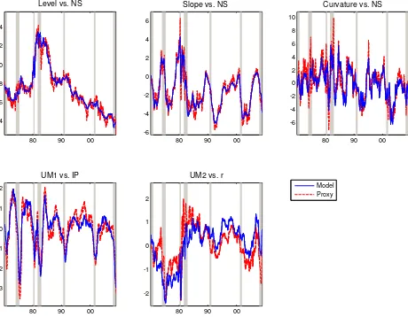
Figure 1 displays the estimated factors of the macro-yields model. The top three plots report
the yield curve factors, while the bottom two refer to the unspanned factors. The estimated yield
curve factors of the macro-yields model are highly correlated with the NS factors, which we estimate
by ordinary least squares as in Diebold and Li (2006) and report in dashed red lines in the top
plots. The differences between the NS factors and the first three macro-yields factors are due to the
fact that, in the macro-yields model, the yield curve factors are common to both yield curve and
macroeconomic variables. In fact, in the macro-yields model, we extract the yield curve factors from
both yields and macroeconomic variables and impose the NS restrictions on the factors loadings
of the yields to identify them as yield curve factors. The two bottom plots of Figure 1 show the
unspanned macro factors. The bottom left plot reports the first unspanned macro factor along
with the industrial production index, while the bottom right plot reports the second unspanned
macroeconomic factor along with the real interest rate (computed as the difference between the
federal funds rate and the consumer price index). As it is clear from the plots, the first unspanned
macroeconomic factor closely tracks the industrial production index, with a correlation of 90%, and
the second unspanned macroeconomic factor proxies the real interest, with a correlation of 74%.
This is in line with the fact that, as reported in Table 2, the first unspanned macroeconomic factor
explains mainly measures of real economic activity, while nominal variables are explained partly
by the yield curve factors and partly by the second unspanned factor. We can thus conclude that
the macro-yields models identifies two unspanned macroeconomic factors: real economic activity
and real interest rate. In the next Section we assess the quantitative importance of the unspanned
6The two macroeconomic factors are not identified since any transformationHFx
Figure 1: Macro-yields factors
80 90 00
4 6 8 10 12 14
Level vs. NS
80 90 00
-6 -4 -2 0 2 4 6
Slope vs. NS
80 90 00
-6 -4 -2 0 2 4 6 8 10
Curvature vs. NS
80 90 00
-3 -2 -1 0 1 2
UM1 vs. IP
Model Proxy
80 90 00
-2 -1 0 1 2
UM2 vs. r
macroeconomic factors in explaining bond risk premia.
4.2 Bond risk premia
The bond risk premium measures the compensation required by risk averse investors to hold
long-term government bonds for facing capital loss risk, if the bond is sold before maturity.
Long-term yields are determined by market expectations for the short rates over the holding
period of the long-term asset plus a yield risk premium. Assuming a minimum investment horizon
of one year, we have
y(tτ)=τ 12
−1
X
i=0,12,...,τ−12
Et[y(12)t+i ] +yrp(tτ). (9)
An alternative measure for the bond risk premium can be obtained by looking at bond returns.
The one-year holding period bond return for a bond with maturityτ months is the return of buying
a bond withτ months to maturity at timet, selling it one year later, at timet+ 12, as a bond with
τ−12 months to maturity, i.e.
rt(+12τ) =−(τ−12)yt(+12τ−12)+τ yt(τ). (10)
The expected one-year holding period return on long term bonds equals the expected return on
short term bond plus the return risk premium
Et[rt(+12τ) ] =y (12)
t +rrp
(τ)
t , (11)
accordingly the return risk premium is the one-year expected return in excess of the one-year rate
rrp(tτ)=Et[r(tτ+12) ]−y (12)
The relation between the return risk premium and the yield risk premium is as follows
yrp(tτ)= 1 τEt
h
rrp(tτ)+rrp(tτ+12−12)+. . .+rrp(24)t+τ−24i, (13)
which means that the yield risk premium is the average of expected future return risk premia of
declining maturity. This implies that the statements in Equations (9) and (11) are equivalent, if
one equation holds with zero (constant) bond risk premium, the other equation holds with zero
(constant) bond risk premium as well.
The expectations hypothesis of the term structure of interest rates states that the yield risk
premium is constant. This implies that expected excess returns are time invariant and, thus, excess
bond returns should not be predictable with variables in the information set at timet. However, the
expectations hypothesis has been empirically rejected since Fama and Bliss (1987) and Campbell
and Shiller (1991). They find that excess returns can be predicted by forward rate spreads and by
yield spreads, respectively. More recent evidence by Cochrane and Piazzesi (2005) shows that a
linear combination of forward rates (the CP factor) explains between 30% and 35% of the variation
in expected excess bond returns. Moreover, Ludvigson and Ng (2009) find that macroeconomic
factors constructed as linear and non-linear combinations of principal components extracted from
a large data-set of macroeconomic variables (the LN factor) have important forecasting power for
future excess returns on U.S. government bonds, above and beyond the predictive power contained
in forward rates and yield spreads. Cooper and Priestley (2009) also find that the output gap has
in-sample and out-of-sample predictive power for U.S. excess bond returns.
The top panel of Figure 2 shows the 5 years to maturity yield along with the corresponding
components as in Equation (9), where the sum of expectations is the sum of forecasts produced
with our macro-yields model and the risk premium is the difference between the 5 years to maturity
yield and the sum of the forecasts of the 1 year to maturity yields. The expectation component
is larger than the risk premium but the graph shows that there is substantial variation of the
Figure 2: Yield risk premium, 5-year bond
72 75 77 80 82 85 87 90 92 95 97 00 02 05 07 0
5 10 15
Yield Expectations MY Risk Premium MY
72 75 77 80 82 85 87 90 92 95 97 00 02 05 07 -2
0 2 4
Risk Premium MY IP Growth
72 75 77 80 82 85 87 90 92 95 97 00 02 05 07 -1
0 1 2 3 4
Risk Premium MY Risk Premium OY
graph plots the risk premium against the industrial production index growth and it reveals that the
yield risk premium obtained from the macro-yields model displays a clear counter-cyclical pattern.
Its correlation with the industrial production index growth is -0.33. This is consistent with the
fact that investors want to be compensated for bearing risks related to recessions. Conversely, the
bottom graph in Figure 2, shows the risk premium obtained from the only-yields model. This model
delivers an acyclical risk premium, with a correlation of only -0.07 with the industrial production
index growth. This indicates that using macro variables greatly improves the estimates of the risk
premium.
Given that, as shown in Equation (13), the yield risk premium is the average of expected future
return risk premia of declining maturity, we analyze the predictive ability of the macro-yields model
for excess returns and compare it with the predictions of the only-yields model. We also compare
our results with predictions obtained using the CP factor, the LN factor and the CP and LN factors
combined.
We implement predictive regressions for the CP and LN factors by regressing excess bond
returns on the predictive factorsXt={CPt, LNt}, as follows
rx(tτ+12) =βXt+ε(tτ+12) . (14)
We construct the predictive factors Xt by pooling the predictive regression for the individual ma-turities
rxt+12=γxt+εt+12, (15)
where rxt+12 = 14Pτ=24,36,48,60rx(tτ+12) and xt contains the predictor variables. To construct the CP factor we use the following predictor variables xCPt = [1, y(12)t , ft(24), . . . , ft(60)], where ft(τ) denotes the τ-month forward rate.7 We estimate equation (15) using xCP
t as predictor variables
7Theτ-month forward rate for loans between timet+τ
−12 andt+τ is defined as
ft(τ)=−(τ−12)y (τ−12) t +τ y
Table 3: In-sample fit of excess bond returns
Maturity MY OY CP LN LN+CP 2y 0.55 0.12 0.22 0.33 0.41 3y 0.53 0.12 0.24 0.33 0.43 4y 0.50 0.14 0.27 0.32 0.43 5y 0.46 0.15 0.24 0.30 0.40 This table reports theR2 for one-year ahead one year holding period excess bond returns from different mod-els. The columns MY and OY refer to the model-implied expected excess bond returns from the macro-yields model (MY) and the only-macro-yields model (OY) re-spectively. The columns CP, LN and CP+LN refer to the predictive regression using the Cochrane and Piazzesi (2005) factor (CP), the Ludvigson and Ng (2009) factor (LN), and both the Cochrane and Pi-azzesi (2005) and the Ludvigson and Ng (2009) factors jointly.
and construct the CP factor as CPt = ˆγCPxCPt . To construct the LN factor, we use as predictor variables xLNt = [1, P C1t, . . . , P C8t, P C13t], where PC denotes principal components extracted from a large dataset of 131 macroeconomic data series.8 We then estimate equation (15) usingxLNt as predictor variables and construct the LN factor as LNt= ˆγLNxLNt .
Notice that the LN factors are constructed aggregating principal components extracted from a
set of macroeconomic and financial variables without imposing that they are unspanned by the cross
section of the yields similarly to the factors extracted by assuming a block-diagonal structure on
the factor loadings. As a consequence, those factors duplicate information that is already spanned
by the yield factors.9
Results in Table 3 show that the macro-yields model explains about 46-55% of the variation
of one-year ahead excess returns, while the only-yields model can explain only the 12-15% of
the variation of the one-year ahead excess returns. Table 3 reports also the R-squared from the
predictive regressions of excess bond returns on the CP and the LN factors. Results show that the
CP factor explains 22-27% of the variation in one-year ahead excess returns, slightly lower than
8The 131 macroeconomic data series used to construct the LN factor have been downloaded from Sydney C.
the value reported in Cochrane and Piazzesi (2005). This is due to the fact that our predictive
regressions are estimated on a more updated sample, and the performance of the CP factor has
deteriorated over time, as also shown by Thornton and Valente (2012). The LN factors explain a
third of the variation of future excess bond returns, while the CP and LN factors jointly explain
40-43% of the variation in one-year ahead excess bond returns, lower than what is explained by our
macro-yields model. We can thus conclude that, in-sample, the macro-yields model outperforms
the CP and the LN factors even combined.
Figure 3 shows the predicted and realized average excess bond returns from the macro-yields
and the only-yields model, and also from the predictive regressions using the CP and the LN factors.
The figure shows that the predicted excess bond returns from the only-yields model are quite flat,
indicating that the yield curve factors poorly predict excess bond returns. The CP factor seems
doing a better job than the only-yields model, but does not improve over the macro-yields model.
The macro-yields model is able to better predict the average excess return, also with respect to the
LN factor.
4.3 Unspanning conditions
Results in the previous section show that the unspanned macro factors play an important role in
explaining the term premium, despite being constrained to not affect current yields. In the context
of Equation (9), this can only happen if the unspanned macro factors have offsetting effects on
average expected future short rates and term premia, see Duffee (2011b).
To understand whether our macro factors are truly unspanned by the yield curve, we compute
the risk premium of an unrestricted macro-yields model which does not impose the zero restriction
on the factor loadings of the yields on the macro factors, i.e. Γyx 6= 0 in Equation (4).10 The estimates of the bond premium delivered by this model are practically indistinguishable from the
estimates obtained using the macro-yields model which instead imposes the restriction Γyx = 0
(the correlation between the estimates is 0.99). The fact that imposing the unspanning restrictions
Figure 3: Average 1-year holding period excess return: realized and predicted
75 80 85 90 95 00 05 −10 −8 −6 −4 −2 0 2 4 6 8 10 rx MY
75 80 85 90 95 00 05 −10 −8 −6 −4 −2 0 2 4 6 8 10 rx OY
75 80 85 90 95 00 05 −10 −8 −6 −4 −2 0 2 4 6 8 10 rx CP
75 80 85 90 95 00 05 −10 −8 −6 −4 −2 0 2 4 6 8 10 rx LN
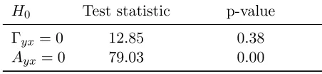
Table 4: Likelihood ratio test statistic for the unspanning restrictions
H0 Test statistic p-value
Γyx= 0 12.85 0.38 Ayx= 0 79.03 0.00
This table reports the likelihood ratio test statistic for the unspanning restrictions and the correspond-ing p-values, computed uscorrespond-ing a chi-squared distribu-tion with degrees of freedom equal to the number of restrictions tested. The first line refers to the null hypotheses Γyx= 0 in Equation (4) while the second line refers to the null hypotheses Ayx = 0 in Equa-tion (5).
has no effect on the yield risk premium indicates that the macro factors are unspanned by the
yield curve. In practice, this means that, in periods of recession, the unspanned macro factors
increase the risk premium and decrease the expected future short rates by the same amount,
without contributing to a steepening of the current yield curve. Conversely, in periods of economic
expansion, the unspanned macro factors decrease the bond premium and increase the expected
future short rates by the same amount, without contributing to a flattening of the current yield
curve. Changes in the current shape of the yield curve can only be determined by changes in the
yield curve factors.
To formally test for the unspanning properties in the context of our state-space macro-yields
model, we define a factor as unspanned by the yield curve if it satisfies the following two conditions.
First, it doesn’t affect the current cross-section of yields, i.e. it is not loaded contemporaneously
by the yields (Γyx= 0 in Equation (4)). Second, it has predictive ability for the yield curve factors (Ayx 6= 0 in Equation (5)), see also Joslin et al. (2014).
The unspanning conditions can be tested performing likelihood ratio tests, as follows
LR= 2×(Lu−Lr) (16)
factor loadings, Lu denotes the loglikelihood of an unrestricted macro-yield model that does not impose the restriction Γyx = 0 and Lr is the loglikelihood of our macro-yields model. The test statistic in Table 4 shows that we cannot reject the null of zero factor loadings of the yields on the
macro factors. This implies that, indeed, the macro factors do not affect the current shape of the
yield curve.11
To test the predictive ability of the macro factors obtained from macro-yields model in
Equa-tions (4)–(6) for the yield factors, and therefore the yield curve of interest rates, we perform the
likelihood ratio test statistics in Equation (16), where, in this case, Lu is the loglikelihood of our macro-yield model and Lr is the restricted loglikelihood obtained imposing Ayx = 0 in Equation (5). Results in Table 4 show that we can reject the null hypothesis of no Granger causality from
the macro factors to the yield curve factors.
These testing results show that the macroeconomic factors identified by the macro-yields model
do not explain the cross-section of yields but have predictive ability for the future evolution of the
yield curve. As a consequence, they satisfy both conditions for being truly unspanned
macroeco-nomic factors. Moreover, looking at the coefficients and their relative standard errors, available in
Appendix F, we can infer that the first unspanned factor, proxied by economic growth, Granger
causes the slope and the curvature, while the second unspanned factor, proxied by the real interest
rate, Granger causes the level.
5
Out of sample forecast
To evaluate the predictive ability of the macro-yields model, we generate out-of-sample iterative
forecasts of the factors, as follows
Et(Ft∗+h)≡Fˆt∗+h|t= ( ˆA∗|t)hFˆt∗|t,
whereh denotes the forecast horizon and ˆA∗|t is estimated using the information available till time t.12 We then compute out-of-sample forecasts of the yields given the projected factors, in this way
Et(zt+h)≡zˆt+h|t= ˆΓ∗|tFˆt∗+h|t.
where ˆΓ∗|t is estimated using data up to timet.
Collecting the excess returns for bonds with maturities from two to five years in the vectorrxt. We compute the out-of-sample predictions of excess bond returns as follows
Et(rxt+12)≡rxt+12|t= Π1yt+12|t+ Π2yt= Π1(ˆΓ∗|tFt∗+12|t) + Π2yt, (17)
where Π1 =
D[−1:−K] 0[K×1]
, Π2 =
−1[K×1] D[2:K+1]
, D[−1:−K] denotes a diagonal matrix with elements −1,−2, . . . ,−K in the diagonal and K + 1 denotes the total number of
maturities. Notice that Equation (17) implies that the forecast errors made in forecasting the
excess returns are proportional to the ones made in forecasting the yields, i.e. rxt+12|t−rxt+12=
Π1(yt+12|t−yt+12), see Carriero, Kapetanios and Marcellino (2012).
We forecast yields and excess returns recursively using data from January 1970 until the time
that the forecast is made, beginning in January 1990 to December 2008.
5.1 Yields
To evaluate the prediction accuracy of the macro yields model for out of sample forecasts of yields,
we use the Mean Squared Forecast Error (MSFE), i.e. the average squared error in the evaluation
period for theh-months ahead forecast of the yield (or excess return) with maturity τ
MSFEt1
t0(τ, h, M) =
1 t1−t0+ 1
t1
X
t=t0
ˆ
yt(τ+)h|t(M)−yt(+τ)h2, (18)
12See Appendix A for the definitions ofF∗
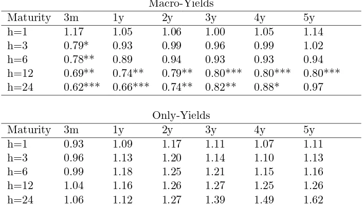
Table 5: Out-of-sample performance for yields
Macro-Yields
Maturity 3m 1y 2y 3y 4y 5y
h=1 1.17 1.05 1.06 1.00 1.05 1.14 h=3 0.79* 0.93 0.99 0.96 0.99 1.02 h=6 0.78** 0.89 0.94 0.93 0.93 0.94 h=12 0.69** 0.74** 0.79** 0.80*** 0.80*** 0.80*** h=24 0.62*** 0.66*** 0.74** 0.82** 0.88* 0.97
Only-Yields
Maturity 3m 1y 2y 3y 4y 5y
h=1 0.93 1.09 1.17 1.11 1.07 1.11 h=3 0.96 1.13 1.20 1.14 1.10 1.13 h=6 0.99 1.18 1.25 1.21 1.15 1.16 h=12 1.04 1.16 1.26 1.27 1.25 1.26 h=24 1.06 1.12 1.27 1.39 1.49 1.62 This table reports the relative MSFE of the macro-yields model and the only-yields model over the MSFE of the random walk for multi-step predictions of the yields. The first column reports the forecast horizonh. The sample starts on January 1970 and the evaluation period is January 1990 to December 2008. *, ** and *** denote significant outperformance at 10%, 5% and 1% level with respect to the random walk according to the White (2000) reality check test with 1,000 bootstrap replications using an average block size of 12 observations.
where t0 and t1 denote, respectively, the start and the end of the evaluation period, yt(+τ)h is the
realized yield with maturityτ at timet+h and ˆyt(+τ)h|t(M) is the h-step ahead forecast of the yield with maturityτ from modelM using the information available up to t.
Forecast results for yields are usually expressed as relative performance with respect to the
random walk, which is a na¨ıve benchmark for yield curve forecasting very difficult to outperform,
given the high persistency of the yields. The random walk h-steps ahead prediction at time t of
the yield with maturityτ is
Et(y(t+τ)h)≡yˆt(+τ)h|t=yt(τ),
where the optimal predictor does not change regardless of the forecast horizon. To measure the
Figure 4: 12-months ahead smoothed squared forecast errors for yields
95 97 00 02 05 07 0 0.5 1 1.5 2 2.5 3 3.5
Maturity 3 months
MY RW
95 97 00 02 05 07 0 0.5 1 1.5 2 2.5 3 3.5
Maturity 3 months
OY RW
95 97 00 02 05 07 0 0.5 1 1.5 2 2.5
Maturity 36 months
MY RW
95 97 00 02 05 07 0 0.5 1 1.5 2 2.5
Maturity 36 months
OY RW
95 97 00 02 05 07 0
0.5 1 1.5 2
Maturity 60 months
MY RW
95 97 00 02 05 07 0
0.5 1 1.5 2
Maturity 60 months
OY RW
MSFE computed as
rMSFEt1
t0(τ, h, M) =
MSFEt1
t0(τ, h, M)
MSFEt1
t0(τ, h, RW)
.
Table 5 reports the rMSFE with respect to the random walk for the macro-yields model the
only-yields model. Results in Table 5 show that the only-yields model is outperformed by the
macro-yields model for all but the 1-month horizon. Moreover, the macro-yields model
outper-forms the random walk at 3-, 6-, 12- and 24-month ahead for all the maturities, with significant
outperformance according to the White (2000) reality check test for the 12- and 24-month ahead
forecasts.13 This evidence is corroborated by Figure 4, which reports the 12-month ahead smoothed
squared forecast errors of the macro-yields, the only-yields and the random walk models for yields
with 3-, 36- and 60-month to maturity. The figure highlights how the macro-yields model has been
systematically outperforming the random walk, especially in the last part of the evaluation sample
for the short maturity and the first part of the sample for long maturities. The only-yield model,
instead has been performing as the random walk in the first part of the evaluation sample but its
performance deteriorated in the last part of the evaluation sample, significantly underperforming
the random walk. This indicates that the unspanned macroeconomic factors, while not important
for explaining the contemporaneous yields curve, contain useful information to predict the future
yield curve factors and, thus, the future evolution of the yield curve.
5.2 Excess bond returns
Out of sample forecast results for excess bond returns are reported in Table 6, which contains
the relative MSFE of the macro-yields model (MY) with respect to the constant excess return
benchmark, where one-year holding period excess returns are unforecastable at one year horizon, as
in the expectation hypothesis. We use the expectation hypothesis since, because of its simplicity,
represents a benchmark of unpredictability. The macro-yields model outperforms the constant
excess return benchmark for all maturities and the outperformance is significant for all maturities
according to the White (2000) reality check test.
Figure 5: Smoothed mean squared forecast errors for excess bond returns
95 97 00 02 05 07
0 5 10 15 20
EH MY
95 97 00 02 05 07
0 5 10 15 20
EH OY
95 97 00 02 05 07
0 5 10 15 20
EH CP
95 97 00 02 05 07
0 5 10 15 20
EH LN
Table 6: Out-of-sample predictive performance for excess returns
Maturity MY OY CP LN LN+CP 2y 0.76** 1.20 1.17 0.80 0.80 3y 0.75** 1.20 1.21 0.79 0.83 4y 0.74** 1.18 1.21 0.78 0.83 5y 0.75** 1.18 1.18 0.81 0.83 This table reports the relative MSFE of the macro-yields model (M Y), the only-yields model (OY), the Cochrane and Piazzesi (2005) factor (CP), the Ludvig-son and Ng (2009) (LN) factor, the Cochrane and Pi-azzesi (2005) and the Ludvigson and Ng (2009) factors combined (LN+CP) with respect to the expectation hy-pothesis for excess returns. The sample starts on January 1970 and the evaluation period is January 1990 to De-cember 2008. * and ** denote significant outperformance at 10% and 5% level with respect to the expectation hy-pothesis according the White (2000) reality check test with 1,000 bootstrap replications using an average block size of 12 observations.
Table 6 also reports the out-of-sample relative MSFEs of the excess bond returns forecasts using
the CP factor, the LN factor, and the CP and LN factors combined obtained from the predictive
regressions in (14). The worst performing models are the ones that do not use macroeconomic
variable, i.e. the only-yield model and the CP factors. In line with the predictive regressions
of excess bond returns and with the 12-month ahead out-of-sample forecast performance of the
macro-yields model for the yields, results in Table 6 show that the macro-yields model is the best
performing model for the prediction of the 1-year excess bond returns for all maturities followed by
the combination of the CP and LN factors. However, although the unspanned model significantly
outperforms the na¨ıve benchmark while the CP+LN does not, we cannot reject the hypothesis that
the forecasts of these two models are statistically equally accurate.
To further understand the performance of the macro-yields model to predict 1-year holding
period excess bond returns, Figure 5 plots the 5-year rolling mean squared forecast error of the
macro-yields model, the only-yields model, the CP and LN factors along with the 5-year rolling
mean squared forecast error under the expectation hypothesis (EH). The figure shows that the
expectation hypothesis in the first part of the evaluation sample but display large forecast errors in
the second part. Also the performance of the macro-yields model and the LN factors are similar,
they both provide more accurate predictions than the expectation hypothesis, in particular in
the last part of the evaluation period. However, it is clear from the figure that the macro-yields
model, apart from being the best performing model on average, as shown in Table 6, it is the best
performing model for the whole evaluation period. This is a clear evidence that the unspanned
macroeconomic factors identified by the proposed macro-yields model as related with economic
growth and real interest rates have predictive ability for the yield curve factors and, thus, for
excess bond returns.
6
Conclusions
In this paper we analyze the predictive content of macroeconomic information for the yield curve of
interest rates and excess bond returns in the United States. We find that two macroeconomic factors
characterizing economic growth and real interest are unspanned by the cross-section of government
bond yields and have significant predictive power for the bond yields and excess returns.
In future research, we plan to extend our empirical specification to allow for the zero lower
bound of interest rates, non-synchronicity of macroeconomic data releases and mixed frequencies.
The macro-yields model presented in this paper cannot be estimated on a sample that includes the
great recession, as it does not ensure a zero lower bound on interest rates. Our model model can,
however, be easily extended to deal with this issue by anchoring the shorter end of the yield curve
using market expectation, along the lines of Altavilla, Costantini, Giacomini and Ragusa (2012).
Data revisions and jagged edges due to the non-synchronicity of macroeconomic data releases
are important characteristics to be taken into account when extracting macroeconomic information,
see Giannone, Reichlin and Small (2008). In addition, bond yields are available at higher frequencies
than macroeconomic variables. These features can be easily incorporated into our empirical model
A
Estimation procedure
We can rewrite the macro-yields model in equations (4)–(6) in compact form as
zt = a+ ΓFt+vt, (19) Ft = µ+AFt−1+ut, ut∼N(0, Q) (20)
vt = Bvt−1+ξt, ξt∼N(0, R) (21)
wherezt= yt xt ,Ft=
Fty Ftx
,a=
0 ax , Γ =
Γyy Γyx Γxy Γxx
,A=
Ayy Ayx Axy Axx
,Q=
Qyy Qyx Qxy Qxx , µ= µy µx
and Γyy = ΓN S is the matrix whose rows correspond to the smooth patterns proposed by Nelson and Siegel (1987) and shown in equation (2). In addition Γyx = 0, as the macroeconomic factors Ftx are unspanned by the cross-section of yields Γyx = 0. We also estimate the only-yields model using the same procedure, as it implies the following restrictions in (19)–(20): zt=yt, Ft= Fty, a= 0,Γ = ΓN S, µ=µy.
The macro-yields model in (19)–(20) can be put in a state-space form augmenting the statesFt with the idiosyncratic componentsvt and a constant ctas follows
zt = Γ∗Ft∗+vt∗, vt∗∼N(0, R∗) Ft∗ = A∗Ft∗−1+u∗t, u∗t ∼N(0, Q∗)
where Γ∗ =
Γ a IN
,Ft∗= Ft ct vt
,A∗=
A µ . . . 0 ..
. . .. 1 ...
0 . . . B
,u∗t = ut νt ξt
,Q∗ =
Q . . . 0 ..
. ε ...
0 . . . R
The restrictions on the factor loadings Γ∗ and on the transition matrix A∗ can be written as
H1 vec(Γ∗) =q1, H2 vec(A∗) =q2,
whereH1 and H2 are selection matrices, and q1 and q2 contain the restrictions.
We assume that F1∗ ∼ N(π1, V1), and define y = [y1, . . . , yT] and F∗ = [F1∗, . . . , FT∗]. Then denoting the parameters byθ={Γ∗, A∗, Q∗, π1, V1}, we can write the joint loglikelihood of zt and Ft, fort= 1, . . . , T, as
L(z, F∗;θ) = − T X
t=1
1
2[zt−Γ
∗F∗
t]′(R∗)−1[zt−Γ∗Ft∗]
+
−T
2 log|R
∗| − T X t=2 1 2[F
∗
t −A∗Ft∗−1]′(Q∗)−1[Ft∗−A∗Ft∗−1]
+
−T −2 1log|Q∗|+1 2[F
∗
1 −π1]′V1−1[F1∗−π1] +
−12log|V1| −
T(p+k)
2 log 2π+λ
′
1(H1vec(Γ∗)−q1) +λ′2(H2vec(A∗)−q2)
where λ1 contains the lagrangian multipliers associate with the constraints on the factor loadings
Γ∗ and λ2 contains the lagrangian multipliers associated with the constraints on the transition
matrixA∗.
The computation of the Maximum Likelihood estimates is performed using the EM algorithm.
Broadly speaking, the algorithm consists in a sequence of simple steps, each of which uses the
Kalman smoother to extract the common factors for a given set of parameters and multivariate
regressions to estimate the parameters given the factors. In practice, we use the restricted version of
the EM algorithm, the Expectation Restricted Maximization, since we need to impose the smooth
pattern on the factor loadings of the yields on the NS factors. The ERM algorithm alternates
Kalman filter extraction of the factors to the restricted maximization of the likelihood. At thej-th
iteration the ERM algorithm performs two steps:
the estimates from the previous iteration, i.e.
L(θ) =E[L(z, F∗;θ(j−1))|z]
which depends on three expectations
ˆ
Ft∗ ≡ E[Ft∗;θ(j−1)|z] Pt ≡ E[Ft∗(Ft∗)′;θ(j−1)|z]
Pt,t−1 ≡ E[Ft∗(Ft∗−1)′;θ(j−1)|z]
These expectations can be computed, for given parameters of the model, using the Kalman
filter.
2. In the Restricted Maximization-step, we update the parameters maximizing the expected
log-likelihood with respect toθ:
θ(j) = arg max θ L(θ)
This can be implemented taking the corresponding partial derivative of the expected log
likelihood, setting to zero, and solving.
The procedure outlined above can be extended to estimate also the decay parameterλcontrolling
for the shape of the loadings of the yields on the slope and curvature factors. Since the factor
loadings are a non-linear function λ, an additional step consisting in the numerical maximization
of the conditional likelihood with respect toλ is required. The procedure is know as Expectation
B
Data
Table 7: Macroeconomic variables
Series N. Mnemonic Description Transformation
1 AHE Average Hourly Earnings: Total Private 1
2 CPI Consumer Price Index: All Items 1
3 INC Real Disposable Personal Income 1
4 FFR Effective Federal Funds Rate 0
5 HSal House Sales - New One Family Houses 1
6 IP Industrial Production Index 1
7 M1 M1 Money Stock 1
8 Manf ISM Manufacturing: PMI Composite Index (NAPM) 0
9 Paym All Employees: Total nonfarm 1
10 PCE Personal Consumption Expenditures 1 11 PPIc Producer Price Index: Crude Materials 1 12 PPIf Producer Price Index: Finished Goods 1 13 CU Capacity Utilization: Total Industry 0
14 Unem Civilian Unemployment Rate 0
This table lists the 14 macro variables used to estimate the macro-yields. Most series have been transformed prior to the estimation, as reported in the last column of the table. The transformation codes are: 0 = no transformation and 1 = annual growth rate.
C
Reality check test
To compare the out of sample predictive ability of a model with respect to the benchmark, we use
the reality check test of White (2000), as we compare only non-nested models.
If we denote by et(b) the forecast errors of the benchmark and by et(M) the forecast errors of the model under consideration. Then we can define the null hypothesis of no predictive superiority
over the benchmark as
H0 :f =E(ft)≡E(et(b)2−et(M)2)≤0 (22)
The test is then based on the statistic
f = 1 t1−t0
t1
X
t=t ˆ
wheret0andt1 denote, respectively, the start and the end of the evaluation period, and hats denote
estimated statistics.
To approximate the asymptotic distribution of the test statistic, we use block-bootstrap as
follows:
1. We generate bootstrapped forecast errors ˆe∗t(b) and ˆe∗t(M) using the stationary block-bootstrap of Politis and Romano (1994) with average block size of 12. This procedure is analogous to
the moving blocks bootstrap, but, instead of using blocks of fixed length uses blocks of
ran-dom length, distributed according to the geometric distribution with mean block length 12.
Also to give the same probability of resampling to all observations, we use a circular scheme.
2. Construct the bootstrapped test statistic as
f∗= 1 t1−t0
t1
X
t=t0
(ˆe∗t(b)2−eˆ∗t(M)2)
3. Repeat steps 1 and 2 for 1,000 times to obtain an estimate of the distribution of the test
statisticf∗ = [f∗(1), . . . , f∗(1,000)].
4. Compare V = (t1−t0)1/2f with the quantiles of V∗ = (t1 −t0)1/2(f
∗
−f) to obtain the
D
Unrestricted vs block-diagonal macro-yields model
In this Appendix we report results for two alternative macro-yields models that use different
as-sumptions about the matrix of factor loadings Γ in Equation (4). The first model that we consider
is an unrestricted macro-yields model, which does not impose the zero restrictions on the factor
loadings of yields on macro factors, i.e. Γyx is allowed to be different from zero. This model
al-lows the macro factors Ftx to directly affect the cross-section of yields. The second model imposes block-diagonality of the matrix of factor loadings Γ, i.e. Γyx = 0 and Γxy = 0. This implies that the yield curve factors and the macro factors are treated separately, as in M¨onch (2012). Notice
that when estimating the block-diagonal macro-yields model, we omit the federal funds rate from
the macro variables used to estimate the model, as in M¨onch (2012). The reason is that we cannot
reliably impose a zero restriction on the factor loadings of the federal funds rate on the yield curve
factors.
Results in Tables 8–11, show that the in-sample and out-of-sample performances of the
unre-stricted macro-yields model are equal to the ones of the macro-yields model with unspanned macro
factors in Tables 2–6. This provides evidence that the zero restrictions on the factor loadings are
satisfied by the data, implying that the macro factors Ftx are unspanned by the cross-section of yields.
On the contrary, imposing a block-diagonal structure on the matrix of factor loadings has
substantial implications for the the identification of the factors. Table 8 shows that the information
criterion selects the model with six factors, i.e. three yield curve factors and three macro factors.
This indicates that this model is less parsimonious than our macro-yields model. In addition, as
shown in Table 9, the macro factors in the block-diagonal macro-yield model are highly correlated
with the yield curve factors and are, thus, spanned by the cross-section of yields. This happens
because the macro variables have a factor in common with the yields which the block-diagonal
model treats as an additional macro factor. Table 9 also shows that the correlation of the first
Table 8: Model selection
Unrestricted Block-diagonal Number of factors IC* V IC* V 3 0.02 0.44 1.17 1.36 4 -0.02 0.31 1.30 1.16 5 -0.11 0.22 1.50 1.05 6 0.01 0.18 0.89 0.43 7 0.25 0.17 1.06 0.38 8 0.43 0.16 1.42 0.41 This table reports the information criterion IC*, as shown in Equation (7) and in Equation (8), and the sum of the vari-ance of the idiosyncratic components (divided by NT), V , when different numbers of factors are estimated. The first two columns refer to the unrestricted macro-yields model. The last two columns refer to the block-diagonal macro-yields model.
weaker than in our model. More importantly, the second and third macro factors do not have a
clear-cut interpretation.
Despite the issues with the interpretation of the factors, the fit of the block-diagonal
macro-yields model is comparable to the fit of our macro-macro-yields, as shown in Table 10. However, Table 11
reveals that the lack of parsimony of the block-diagonal macro-yields model leads to out-of-sample
Table 9: Factor identification
Unrestricted
L S C M1 M2
NS L 0.98 0.00 0.32 -0.08 0.01 NS S 0.03 0.97 0.28 0.11 0.08 NS C 0.25 0.37 0.86 0.12 0.06 IP -0.08 0.03 0.16 0.91 -0.09 R 0.47 0.05 0.10 0.20 -0.76
Block-diagonal
L S C M1 M2 M3
Table 10: In sample performance
Unrestricted Model
L S C M1 M2
Average Hourly Earnings:Total Private 0.07 0.29 0.33 0.33 0.67 Consumer Price Index: All Items 0.19 0.48 0.48 0.50 0.86 Real Disposable Personal Income 0.00 0.02 0.03 0.34 0.36 Effective Federal Funds Rate 0.54 0.93 0.96 0.96 0.97 Hose Sales - New One Family Houses 0.00 0.19 0.19 0.22 0.22 Industrial Production Index 0.02 0.02 0.03 0.70 0.70
M1 Money Stock 0.17 0.25 0.25 0.25 0.31
ISM Manufacturing: PMI Composite Index (NAPM) 0.03 0.05 0.05 0.61 0.65 Payments All Employees: Total nonfarm 0.00 0.02 0.10 0.71 0.71 Personal Consumption Expenditures Price Index 0.16 0.23 0.33 0.47 0.79 Producer Price Index: Crude Materials 0.03 0.13 0.13 0.20 0.43 Producer Price Index: Finished Goods 0.03 0.31 0.31 0.32 0.81 Capacity Utilization: Total Industry 0.02 0.16 0.20 0.62 0.63 Civilian Unemployment Rate 0.44 0.53 0.55 0.64 0.67
Block-diagonal Model
L S C M1 M2 M3
Average Hourly Earnings: Total Private 0.00 0.00 0.00 0.09 0.57 0.68 Consumer Price Index: All Items 0.00 0.00 0.00 0.07 0.76 0.76 Real Disposable Personal Income 0.00 0.00 0.00 0.13 0.37 0.42 House Sales - New One Family Houses 0.00 0.00 0.00 0.00 0.07 0.60 Industrial Production Index 0.00 0.00 0.00 0.63 0.80 0.80
M1 Money Stock 0.00 0.00 0.00 0.00 0.05 0.48
Table 11: Out-of-sample performance
Unrestricted
Maturity 3m 1y 2y 3y 4y 5y
h=1 1.21 1.04 1.05 1.01 1.05 1.12 h=3 0.81* 0.93 0.99 0.97 0.99 1.02 h=6 0.79** 0.89 0.95 0.93 0.93 0.94 h=12 0.67** 0.73** 0.78** 0.79*** 0.79*** 0.79*** h=24 0.59*** 0.63*** 0.71*** 0.78*** 0.84** 0.92
Block-diagonal
Maturity 3m 1y 2y 3y 4y 5y
D.1 The block-diagonal model and principal components
This Appendix compares the principal components extracted exclusively from the macroeconomic
variables used in this paper with our unspanned macro factors (top panel), and with the factors
extracted from a macro-yield model with block-diagonal structure (bottom panel).
Table 12 reports the pairwise correlations between the macro-yields factors and the first eight
principal components extracted from our dataset of macro variables. The factors extracted from
the block-diagonal model are very similar to the first three principal components. As stressed in the
paper, this is the consequence of the fact that the block-diagonal model treats the macroeconomic
factors separately from the bond yield factors.
Instead, the unspanned macroeconomic factors are significantly correlated with the first four
principal components. This is not surprising since principal components contains also information
[image:42.612.158.472.417.551.2]that is already spanned by the yield curve.
Table 12: Correlation of principal components with other factors
Unspanned macro-yields factors
PC1 PC2 PC3 PC4 PC5 PC6 PC7 PC8 UM1 0.32 -0.87 0.19 0.04 0.14 0.09 0.04 0.02 UM2 0.63 0.22 0.19 0.44 -0.07 0.17 -0.40 0.16
Block-diagonal macro-yields factors
D.2 LN factor and principal components
This Appendix compares our macro-yields factors with the Ludvigson and Ng (2009) factor and
the principal components used to construct it.
Table 13 reports the pairwise correlations between the our macro-yields factors and the first
eight principal components extracted from a large dataset of 131 variables.14 Results in Table 13
show that the principal components are highly correlated with the yield curve factors extracted
from our macro-yields model. This implies that also the LN factor is highly correlated with the yield
curve factors as it just aggregates information from the principal components without separating
[image:43.612.139.488.350.442.2]the information already spanned by the cross-section of yields.
Table 13: Correlation PC and LN factors with our macro-yield factors
PC1 PC2 PC3 PC4 PC5 PC6 PC7 PC8 LN
L -0.18 0.04 -0.06 -0.26 0.30 -0.12 0.08 0.10 0.05 S -0.20 0.70 -0.23 0.01 0.33 0.08 0.13 0.06 -0.39 C 0.00 0.18 -0.08 0.01 0.08 -0.10 -0.08 0.15 -0.12 UM1 0.71 0.35 -0.06 0.39 0.05 -0.01 -0.09 0.10 -0.58 UM2 0.04 0.18 -0.04 0.04 -0.03 0.07 0.19 -0.10 -0.34
This table reports the correlation of the macro-yields factors with the principal components extracted from a large dataset of macro variables and used to construct the Ludvigson and Ng (2009) factor.
E
Comparison between initial and final estimates
In this Appendix we compare the performance of the initial and the final estimates of the
macro-yields model. The initial estimates of the yield curve factors are computed using the two-steps OLS
procedure introduced by Diebold and Li (2006). We then project the macroeconomic variables on
the NS factors and use the principal components of the residuals of this regression as the initial
estimates of the unspanned macroeconomic factors. These estimated factor are then treated as if
they were the true observed factors. The initial parameters are hence estimated by OLS. The final
estimates are obtained using the EM algorithm where the initial estimates of the factors are used
in order to initialize the algorithm, as described in Section 3 and Appendix A.
Table 14 reports the cumulative variance of yields and macro variables explained by the initial
estimates of the macro-yields factors. Comparing these results with the ones of Table 2, it is clear
that the fit of the initial estimates is at least as good as the fit of the final estimates of the model.
Figure 6 shows the initial estimates of the macro-yields factors are much more volatile than the
final estimates. However, the correlation between the initial estimates and the final estimates of
the macro-yields factors is very high, as shown in Table 15.
The out-of-sample performance of the macro-yields model improves when using the QML
esti-mator compared to the initial estimates obtained by OLS and principal components, see Table 16.
This is due to the fact that the QML estimator take appropriately into account the dynamics of