Dynamic simulation of large-scale power systems using a parallel schur-complement-based decomposition method

White Rose Research Online URL for this paper:

http://eprints.whiterose.ac.uk/105990/

Version: Accepted Version

Article:

Aristidou, P orcid.org/0000-0003-4429-0225, Fabozzi, D and Van Cutsem, T (2014)

Dynamic simulation of large-scale power systems using a parallel

schur-complement-based decomposition method. IEEE Transactions on Parallel and

Distributed Systems, 25 (10). pp. 2561-2570. ISSN 1045-9219

https://doi.org/10.1109/TPDS.2013.252

© 2013 IEEE. This is an author produced version of a paper published in IEEE

Transactions on Parallel and Distributed Systems. Personal use of this material is

permitted. Permission from IEEE must be obtained for all other uses, in any current or

future media, including reprinting/republishing this material for advertising or promotional

purposes, creating new collective works, for resale or redistribution to servers or lists, or

reuse of any copyrighted component of this work in other works. Uploaded in accordance

with the publisher's self-archiving policy.

[email protected] https://eprints.whiterose.ac.uk/

Reuse

Items deposited in White Rose Research Online are protected by copyright, with all rights reserved unless indicated otherwise. They may be downloaded and/or printed for private study, or other acts as permitted by national copyright laws. The publisher or other rights holders may allow further reproduction and re-use of the full text version. This is indicated by the licence information on the White Rose Research Online record for the item.

Takedown

If you consider content in White Rose Research Online to be in breach of UK law, please notify us by

Supplemental Material for “Dynamic Simulation

of Large-scale Power Systems Using a Parallel

Schur-complement-based Decomposition

Method”

Petros Aristidou,

Student Member, IEEE,

Davide Fabozzi, and Thierry Van Cutsem,

Fellow Member, IEEE

F

A

A

D

D

M

DDMs were originally used due to the lack of memory in computing systems: data needed for smaller portions of a problem could fit entirely to the memory while for the whole problem they could not. They lost their appeal as larger and cheaper memory became available, only to resurface in the era of parallel computing. These methods are inherently suited for execution on parallel architectures and many parallel implementations have been presented on multi-core computers, clusters and lately Graphics Processing Units (GPUs) [1], [2].

They are mainly distinguished by three features: sub-domain partitioning, problem solution over sub-sub-domains and sub-domain interface variable processing [3].

A.1 Sub-domain Partitioning

Sub-domain partitioning has to be chosen based on the desired sub-domain characteristics for the given prob-lem. This includes choosing the number of sub-domains, the type of partitioning, and the level of overlap between the sub-domains. Each of these choices depend on a variety of factors such as size, type, and geometry of the problem domain, the number of parallel processors, communication cost, and the actual system being solved. When considering spatial domain problems, such as PDEs, the decomposition is usually given by the geo-metrical data and the order of the discretization scheme used. Conversely, in state domain problems, such as DAE, no a priori knowledge of the coupled variables is available since there are no regular data dependencies. Furthermore, each system model can be composed by

Petros Aristidou is with the Department of Electrical Engineering and Computer Science, University of Liège, Liège, Belgium, e-mail: [email protected].

Davide Fabozzi is with the Department of Electrical Engineering and Computer Science, University of Liège, Liège, Belgium.

Thierry Van Cutsemis with the Fund for Scientific Research (FNRS) at the Department of Electrical Engineering and Computer Science, University of Liège, Liège, Belgium, e-mail: [email protected].

several sub-models which are sometimes hidden, too complex, or used as black boxes. Hence, an automatic decomposition of the system is not trivial [4]. In fact, they usually have to rely on problem specific tech-niques which require good knowledge of the underlying system, the models composing it and the interaction between them.

A.2 Solution and Interface Variable Processing

Each sub-domain problem is then solved exactly or approximately before exchanging information with other sub-domains. The frequency at which information is ex-changed with other sub-domains leads to a compromise between numerical convergence and data exchange rate. Exchanging information frequently leads to faster con-vergence, as sub-domain solution methods always use recent values of interface variables, but higher data exchange rate. Exchanging information infrequently or keeping them constant during the whole solution leads to smaller data exchange rates but might degrade the global convergence as sub-domain solution methods use older interface values. It is obvious that when the sub-domains are weakly connected or disjoint, thus interface variables do not affect strongly the sub-domain solution, infrequent updating is better. This kind of partitioning, though, might be very difficult or even impossible.

The choice on the processing of the interface variables dictates the method used for solving the decomposed problem. The two principle methods are: Schwartz al-ternating and Schur complement.

A.2.1 Schwarz Alternating Method

implementations since the data exchange rate is mini-mum. On the contrary, if the sub-domains are not weakly coupled the algorithm can suffer from degraded conver-gence or even diverconver-gence [5], [6], [7], [8]. Other variants of this method can be found in literature depending on how often and in which order the interface variables are updated, for instance the additive or multiplicative Schwartz procedures [3].

A.2.2 Schur Complement Method

When applying the Schur complement DDM, also called iterative sub-structuring, non-overlapping sub-domain partitioning is employed. The sub-domain problems usu-ally involve interior (coupled only through local equa-tions), local interface (coupled through both local and non-local equations) and external interface (belong to other sub-domains) variables. Next, a numerical method (e.g. Newton’s) is used to solve the sub-problems.

The Schur complement technique is a procedure to eliminate the interior variables in each sub-domain and derive a global, reduced in size, linear system involving only the interface variables. This reduced system is then solved to obtain the interface variables before each sub-domain iterative solution.

Once the interface variables are computed, the sub-problems are decoupled and the remaining, interior to each sub-domain, variables can be computed indepen-dently. In many cases, building and solving the reduced system involves high computational cost. Many methods are used to speed up the procedure, such as approxi-mately solving the system [9], assembling the matrix in parallel using the “local” Schur complements [3], using Krylov solvers [4] or, exploiting the structure of the decomposition to simplify the problem [4], [3].

The formulation and update of the sub-domain solu-tion systems, the eliminasolu-tion of the interior variables, the formulation of the reduced system and the solution of the sub-domain systems can be done in parallel. Unfortunately, this method introduces a bottleneck to the solution algorithm: the sequential computation of the global reduced system to update the interface values. The ratio between the sequential and the parallel part of the algorithm dictates the scalability of the algorithm. However, due to the continuous update of interface variables, the numerical convergence of the algorithm is significantly better than that of Schwarz methods.

A

B

D

S

A

B.1 VDHN Algorithm

One of the most common sequential algorithms used in simulation software [10] is the Very DisHonest Newton (VDHN) which belongs to the quasi-Newton family [11]. The algorithm solves directly the integrated DAE system with the use of a Newton method over discretized time. At each discrete time instant the non-linear DAE equations are discretized and algebraized to acquire a

system of linear equations △ = , where is the Jacobian matrix,y is the vector of unknowns (xandV) andbis the vector of mismatch values of the non-linear, algebraized equations. The linear system is then solved using a sparse linear solver and the values ofyandbare updated. Using the updated values, a new linear system is formulated and solved until the procedure converges. Usually, due to the high computational cost of up-dating the Jacobian matrix J after each solution, the latter is kept constant for many consecutive iterations or even time-steps. If correctly implemented, these methods do not affect the accuracy but only the trajectory of the iterative solution. The convergence of the method can be checked on the computed correction∆y, on the mismatch valuesbor a combination of both. When the method has converged, the solution algorithm proceeds to the next time instant, formulates and solves the new DAE system.

This algorithm is employed by many industrial and academic software and its capabilities and performance are well known. For this reason, it is usually used as the benchmark for proposed algorithms [10].

B.2 Fine-grained Parallel Methods

In order to accelerate the simulation, researchers tried to employ fine-grained parallelization with the use of customized parallel linear solvers. Some methods, like parallel VDHN [12], Newton W-matrix [13] and parallel LU [14], divide the independent vector and matrix op-erations involved in the linear system solution over the available computing units. Other methods, like parallel successive over relaxed Newton [15] and Maclaurin-Newton [12], use an approximate (relaxed) Jacobian ma-trix with more convenient structure for parallelization.

While the fine-grained parallelization methods pro-vide some speedup, they are don’t exploit the full poten-tial of parallel architectures. A more coarse-grained way of exploiting parallelization was sought, and for that, researchers redirected their attention to DDMs.

B.3 Coarse-grained Parallel Methods

As described in App. A, the main idea of DDMs is to partition the original system, into smaller interconnected sub-systems and employ some form of parallel algorithm to solve them. The first to envisage this application on power system was probably Kron [16] with the diakoptics method, where the domain is “teared” into sub-problems, solved independently and joined back together. At the time, parallel computing was not an option and the target was to address memory issues, but, this method provided the ignition for many of the parallel methods to follow.

parallel tasks. Following, several methods were pro-posed inspired by different hardware platforms, mem-ory models and partitioning schemes [2], [19], [20], [21]. Some recently proposed methods make use of both coarse-grained and fine-grained parallelization in a nested way [1] to increase performance. Several charac-teristics differentiate these methods. The most important being the partitioning scheme, the interface variables processing method and the relaxation of interface vari-ables.

As discussed in App. A, automatic partitioning of DAE systems, such as power systems, is not trivial. Some methods, like coherency analysis [22], epsilon decompo-sition [23] and graph partitioning [7] have been proposed in literature, each with its own benefits and problems. The choice of the decomposition plays big role in the speed of convergence, the load balancing among parallel tasks and the overall performance of the method.

A common characteristic of the already proposed decomposition schemes is the partitioning of the net-work to interconnected sub-netnet-works and the applica-tion of Schwartz-based methods for the full paralleliza-tion of the soluparalleliza-tion avoiding the sequentiality of Schur-complement-based methods. This comes at the cost of computing the partition of a network, which can change according to the topology of the system or even the disturbance to be simulated. Moreover, the Schwartz-based treatment of interface variables can initiate several new iterations, especially if partitioned sub-networks are closely coupled [7].

A

C

P

C

C.1 Selecting a Parallel Programming Model

Several options are available when developing a parallel implementation. The main candidates considered for our application were:

• distributed memory model, mainly using Message

Passing Interface (MPI)

• General Purpose computing on GPUs (GPGPU)

• partitioned global address space, mainly using

For-tran Co-array

• shared-memory model, mainly using OpenMP.

The main factors considered to select the appropriate model were: synchronization cost, data exchange rate, hardware cost and easiness to program.

MPI was rejected because its high cost of communi-cation makes it more suitable for coarse-grained parallel algorithms. Algorithms with high rate of data exchange among parallel tasks, as the one proposed, are not likely to be efficient on distributed memory architectures.

GPUs are really good at crunching numbers and can deliver huge peak performance, but they are not as good in handling the irregular computation patterns (unpredictable branches, looping conditions, irregular memory access patterns, etc.) that most engineering soft-ware deal with. Moreover, the CPU to GPU data transfer

link has relatively high latency introducing a significant bottleneck in the execution of the program. Additionally, there is a high effort needed to develop and maintain GPGPU code and low portability as no default standard exists among GPU vendors. Thus, it was rejected.

Co-array was recently introduced in the Fortran stan-dard as an integrated parallel programming model. It was rejected as the existing support by compilers is min-imal and the available user experience and supporting material almost non-existing.

OpenMP, the selected model, is an shared-memory API aiming to facilitate shared-memory parallel pro-gramming. OpenMP is not an official standard but it is supported by most hardware and software vendors and it provides a portable, user-friendly, and efficient approach to shared-memory parallel programming. It is intended to be suitable for a broad range of symmetric multiprocessing architectures.

It consists of a set of compiler directives, library rou-tines, and environment variables that influence run-time behavior. A set of predefined directives are inserted in Fortran, C or C++ programs to describe how the work is to be shared among threads that will execute on different processors or cores and to order accesses to shared data.

C.2 OpenMP Parallel Work Scheduling

OpenMP offers some mechanisms for the assignment of loop iterations to threads through the schedule clause. Very often, the best load balancing strategy depends on the target architecture, the actual data input, and other factors not known at programming time. In the worst case, the best strategy may change during the execution time due to dynamic changes in the behavior of the loop or changes in the resources available in the system. Even for advanced programmers, selecting the best load balancing strategy is not an easy task and can potentially take a large amount of time.

! ! ! ! ! ! ∀

∀

! !

#

! !

∃

! ! ∀

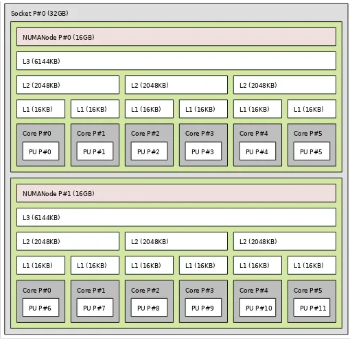
Figure 1. cc-Numa architecture used in our tests

C.3 NUMA Architecture Computers

The proposed implementation targets small and medium, shared-memory parallel computers. Small shared-memory machines (e.g. multi-core laptops and office desktops) have UMA architecture, thus each individual processor can access any memory location with the same speed. On the other hand, larger shared-memory machines usually have NUMA architecture, hence some memory may be “closer to” one or more of the processors and accessed faster by them [24].

The main benefit of NUMA computers over UMA is scalability, as it is extremely difficult to scale UMA computers beyond 8-12 cores. At that number of cores, the memory bus is under heavy contention. NUMA is one way of reducing the number of CPUs competing for access to a shared memory bus by having several memory buses and only having a small number of cores on each of those buses.

The cache coherent NUMA (cc-NUMA) nodes pre-sented in Fig. 1 are part of a 24-core NUMA parallel com-puter, based on 6238 AMD Opteron Interlagos, used in our tests (see Section 5.2, machine (4)). The computer has two identical sockets, each hosting two NUMA nodes with six cores. So, even though the system physically has two CPU sockets with 12 cores each, they are in fact four NUMA nodes with six cores each.

Resources within each node are tightly coupled with a high speed crossbar switch and access to them inside a NUMA node is fast. Moreover, each core has dedicated L1 cache, every two cores have shared L2 cache and the L3 cache is shared between all six cores. These nodes are connected to each other with HyperTransport 3.0 links. The bandwidth is limited to 12GB/s between the two nodes in the same socket and 6GB/s to other nodes.

Parallel applications executing on NUMA computers need special consideration to avoid high overhead costs. First, given the large remote memory access latency, obtaining a program with a high level of data locality is of the utmost importance. Hence, in addition to choosing the appropriate scheduling strategy, some features of the architecture and the OS affect the application’s perfor-mance (binding threads to particular CPUs, arranging the placement and dynamic migration of memory pages, etc.) [24].

Data accessed more frequently by a specific thread should be allocated “close” to that thread. First Touch

memory allocation policy, which is used by many OS, dictates that the thread initializing an object gets the page associated with that item in the memory local to the processor it is currently executing on. This policy works surprisingly well for programs where the updates to a given data element are typically performed by the same thread throughout the computation. Thus, if the data access pattern is the same throughout the application, the initialization of the data should be done inside a parallel segment using the same pattern so as to have a good data placement in memory. This data initializing procedure is followed in our parallel implementation, with each thread initializing the data of the sub-domains statically assigned to it.

Some further consideration is needed when large amount of data are read from files to avoid page mi-gration during the initialization. This problem usually affects NUMA machines with low link speed and appli-cations with intensive i/o procedures. In power system dynamic simulations the data reading is usually done once and then used numerous times to asses several different contingencies on the same system, thus this feature is not critical to their overall performance.

The second challenge on a cc-NUMA platform is the placement of threads onto the computing nodes. If during the execution of the program a thread is migrated from one node to another, all data locality achieved by proper data placement is destroyed. To avoid this we need some method of binding a thread to the processor it was executing during the initialization. In the proposed implementation, the OpenMP environ-ment variableOMP_PROC_BINDis used to prevent the execution environment from migrating threads. Several other vendor specific solutions are also available, like

kmp_affinityin Intel OpenMP implementation,tasksetand

numactl under Linux, pbind under Solaris, bindprocessor

under IBM AIX, etc.

A

D

D

R

A

D.1 Test-case A

0.9 0.91 0.92 0.93 0.94 0.95 0.96 0.97 0.98 0.99

0 40 80 120 160 200 240

Voltage (pu)

Simulation time (s) Algorithm (I) Algorithm (P) Algorithm (EP) 0.968 0.969 0.97 0.971 0.972

102 104 106 108 110 112 114 0.968

0.969 0.97 0.971 0.972

102 104 106 108 110 112 114

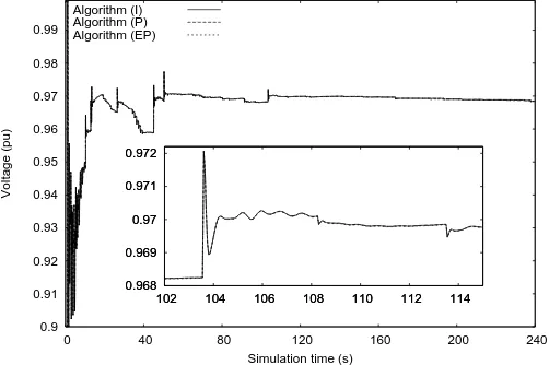
Figure 2. Case A1: Transmission bus voltage

0.8 0.82 0.84 0.86 0.88 0.9 0.92 0.94 0.96 0.98

0 40 80 120 160 200 240

Voltage (pu)

Simulation time (s) Algorithm (I) Algorithm (P) Algorithm (EP) 0.885 0.89 0.895

80 82 84 86 88 90 92 94 96 0.885

0.89 0.895

80 82 84 86 88 90 92 94 96

Figure 3. Case A2: Transmission bus voltage

the short-term dynamics the system starts collapsing but is stabilized in the long-term by the actions of the ASCS devices. Such test-cases are the most computationally demanding as they need to be simulated for the whole time horizon to decide whether the disturbance is criti-cal. Moreover, the actual trajectory of the system states is very important, hence static simulations cannot conclude for their stability.

Figure 3 shows the voltage evolution on the same transmission bus for test-case A2. This time, the system is stable in the short-term but long-term voltage unstable. In test-case A1 the voltage collapse is averted by the actions of the ASCS devices deactivated in A2. All three algorithms provide the same results concerning the stability and response of the test-cases.

Figures 2 and 3 show the same responses simulated with all three algorithms. (P) offers exactly the same response as (I) as they are numerically equivalent. On the other hand, algorithm (EP) shows some small de-viations from the other two (see Figs. 2 and 3, zoom). As explained in Section 3.5, (EP) allows converged sub-domains to stop being computed but keeps checking that they satisfy the convergence criteria throughout the remaining solution. Therefore, its response is almost

1 1.005 1.01 1.015 1.02 1.025 1.03 1.035

0 40 80 120 160 200 240

Voltage (pu)

Simulation time (s) Algorithm (I) Algorithm (P) Algorithm (EP) 1.0205 1.0211 1.0217

20 22 24 26 28 30 1.0205

1.0211 1.0217

20 22 24 26 28 30

Figure 4. Case B: Transmission bus voltage

0.9996 0.9997 0.9998 0.9999 1 1.0001 1.0002 1.0003

0 40 80 120 160 200 240

Machine speed (pu)

Simulation time (s) Algorithm (I) Algorithm (P) Algorithm (EP) 0.9999 1 1.0001

20 22 24 26 28 30 0.9999

1 1.0001

20 22 24 26 28 30

Figure 5. Case B: Generator speed

indistinguishable from the other two and any small de-viations at each discrete time computation are bounded by the convergence tolerance.

D.2 Test-case B

Figures 4 and 5 show the voltage evolution of a trans-mission bus and the machine speed of a synchronous generator, respectively. This test-case exhibits short-term as well as long-term stability. Similarly to test-case A1, this is a marginally stable simulation. That is, after the electromechanical oscillations have died out, the system evolves in the long-term under the effect of LTC de-vices acting to restore distribution voltages. The decision about the stability of the system can only be made after the simulation of the whole time horizon.

A

E

A

S

P

I

E.1 Performance Evaluation

To asses the performance of an existing parallel im-plementation or the potential of a proposed algorithm, Amdahl’s law is often used [25]. It is based on the observation that any parallel implementation consists of a sequentially computed portionSand a parallel portion

P that can be split and assigned to M computational units. Furthermore, it assumes perfect load balancing and a perfect parallel machine without any paralleliza-tion overhead. The most well known variant is:

Runtime(M) =S+ P

M (1)

Of course, the sumP+Shas to account for the sequential execution time of the implementation (M = 1).

Based on (1), the scalability of parallel algorithm can be defined as:

T heoretic scalability(M) = S+P

Runtime(M) (2)

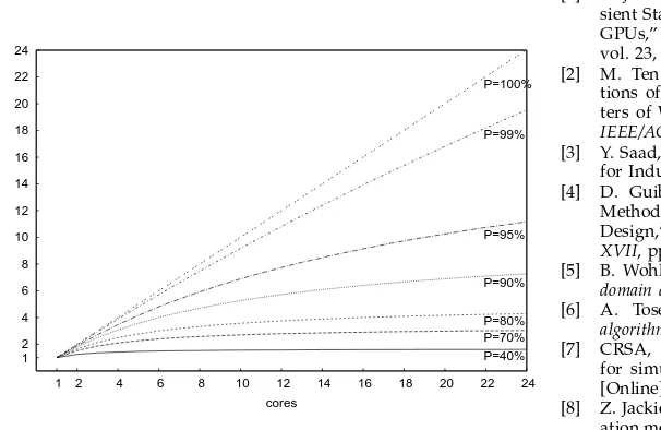
It is called theoretic scalability as it can never be reached in real applications because of parallelization overhead costs, imbalances in load scheduling, etc. Figure 6 dis-plays the theoretic scalability for several percentage val-ues of parallel work P. It is noticeable that even small differences in the percentage of parallel work lead to big differences in the scalability of the algorithm.

To accommodate for overhead cost of making the code run in parallel (managing threads, communication, memory latency, etc.) Amdahl’s law can be modified to:

Runtime(M) =S+ P

M +OHC(M) (3)

where OHC is the overhead cost as a function of the number of computational units used. The modified for-mula can be used to provide a more realistic prediction of scalability and can be directly linked to the formulas presented in Section 5.1.

1 2 4 6 8 10 12 14 16 18 20 22 24

1 2 4 6 8 10 12 14 16 18 20 22 24

Theoretic scalability

cores

P=100%

P=99%

P=95%

P=90%

P=80% P=70% P=40%

Figure 6. Theoretic scalability based on Amdahl’s law

Profiling results: Test-case B / algorithm (P)

% Parallel

Time step initialization 10.02 NO Injector sub-domain discretization

12.51 YES Jacobian calculation and factorization

Schur complement contributions

2.84 YES to simplified reduced system

Factorization and solution of simplified

7.12 NO reduced system (Section 3.3, Eq. 8)

Injector sub-domain solution for interface

61.75 YES and interior variables (Section 3.2, Eq. 4)

Sub-domain convergence check 3.15 YES Various (bookkeeping, etc.) 2.61 NO

Total 100.00% 80.25%

E.2 Profiling Example

Equation 3 shows that scalability can be increased either by increasing the parallel work percentage P or by re-ducing theOHCs. Finally, it can explain situations where increasing the number of available computational units degrades the performance due to increasedOHCs. That is, the value of[P

M − P M+1

]

−[OHC(M + 1)−OHC(M)]

becomes negative.

In Table 1 a sample profiling performed on the se-quential execution of algorithm (P) for test-case B is presented. Consequently, the theoretic scalability on 24 cores can be computed as S+P

S+P

24

= 4.3, with P = 0.8025 the parallel and S = 0.1975 the sequential portion of the implementation as defined in App. E.1. This means that, if the profiled simulation is executed on a24 core parallel computer, without any OHC and with perfect load balancing, a scalability of 4.3 could be expected. This value can be compared to the actual scalability of 3.9 achieved (Section 5.4, Table 3). As expected, the actual scalability is smaller than the theoretical due to the overhead costs discussed in Apps. C.3 and E.1.

R

[1] V. Jalili-Marandi, Z. Zhou, and V. Dinavahi, “Large-Scale Tran-sient Stability Simulation of Electrical Power Systems on Parallel GPUs,” Parallel and Distributed Systems, IEEE Transactions on, vol. 23, no. 7, pp. 1255 –1266, july 2012.

[2] M. Ten Bruggencate and S. Chalasani, “Parallel Implementa-tions of the Power System Transient Stability Problem on Clus-ters of Workstations,” inSupercomputing, 1995. Proceedings of the IEEE/ACM SC95 Conference, 1995, p. 34.

[3] Y. Saad,Iterative methods for sparse linear systems, 2nd ed. Society for Industrial and Applied Mathematics, 2003.

[4] D. Guibert and D. Tromeur-Dervout, “A Schur Complement Method for DAE/ODE Systems in Multi-Domain Mechanical Design,”Domain Decomposition Methods in Science and Engineering XVII, pp. 535–541, 2008.

[5] B. Wohlmuth, Discretization methods and iterative solvers based on domain decomposition. Springer Verlag, 2001.

[6] A. Toselli and O. Widlund, Domain decomposition methods– algorithms and theory. Springer Verlag, 2005.

[7] CRSA, RTE, TE, and TU/e, “D4.1: Algorithmic requirements for simulation of large network extreme scenarios,” Tech. Rep. [Online]. Available: http://www.fp7-pegase.eu/download.html [8] Z. Jackiewicz and M. Kwapisz, “Convergence of waveform

[9] Y. Saad, “Schur complement preconditioners for distributed gen-eral sparse linear systems,” Domain Decomposition Methods in Science and Engineering XVI, pp. 127–138, 2007.

[10] D. Tylavsky, A. Bose, F. Alvarado, R. Betancourt, K. Clements, G. Heydt, G. Huang, M. Ilic, M. La Scala, and M. Pai, “Parallel processing in power systems computation,”Power Systems, IEEE Transactions on, vol. 7, no. 2, pp. 629 –638, may 1992.

[11] J. E. Dennis Jr and J. J. Moré, “Quasi-Newton methods, motivation and theory,”SIAM review, vol. 19, no. 1, pp. 46–89, 1977. [12] J. Chai and A. Bose, “Bottlenecks in parallel algorithms for power

system stability analysis,” Power Systems, IEEE Transactions on, vol. 8, no. 1, pp. 9–15, 1993.

[13] L. Yalou, Z. Xiaoxin, W. Zhongxi, and G. Jian, “Parallel algorithms for transient stability simulation on PC cluster,” inPower System Technology, 2002. Proceedings. PowerCon 2002. International Confer-ence on, vol. 3, 2002, pp. 1592 – 1596 vol.3.

[14] K. Chan, R. C. Dai, and C. H. Cheung, “A coarse grain parallel solution method for solving large set of power systems network equations,” inPower System Technology, 2002. Proceedings. Power-Con 2002. International Power-Conference on, vol. 4, 2002, pp. 2640–2644. [15] J. S. Chai, N. Zhu, A. Bose, and D. Tylavsky, “Parallel newton

type methods for power system stability analysis using local and shared memory multiprocessors,” Power Systems, IEEE Transac-tions on, vol. 6, no. 4, pp. 1539–1545, 1991.

[16] G. Kron, Diakoptics: the piecewise solution of large-scale systems. MacDonald, 1963.

[17] M. Ilic’-Spong, M. L. Crow, and M. A. Pai, “Transient Stability

Simulation by Waveform Relaxation Methods,” Power Systems, IEEE Transactions on, vol. 2, no. 4, pp. 943 –949, nov. 1987. [18] M. La Scala, A. Bose, D. Tylavsky, and J. Chai, “A highly parallel

method for transient stability analysis,” Power Systems, IEEE Transactions on, vol. 5, no. 4, pp. 1439 –1446, nov 1990.

[19] D. Fang and Y. Xiaodong, “A new method for fast dynamic simulation of power systems,”Power Systems, IEEE Transactions on, vol. 21, no. 2, pp. 619–628, 2006.

[20] J. Shu, W. Xue, and W. Zheng, “A parallel transient stability simulation for power systems,”Power Systems, IEEE Transactions on, vol. 20, no. 4, pp. 1709 – 1717, nov. 2005.

[21] V. Jalili-Marandi and V. Dinavahi, “SIMD-Based Large-Scale Tran-sient Stability Simulation on the Graphics Processing Unit,”Power Systems, IEEE Transactions on, vol. 25, no. 3, pp. 1589 –1599, aug. 2010.

[22] D. Koester, S. Ranka, and G. Fox, “Power systems transient stability-a grand computing challenge,” Northeast Parallel Archi-tectures Center, Syracuse, NY, Tech. Rep. SCCS, vol. 549, 1992. [23] A. Zecevic and N. Gacic, “A partitioning algorithm for the parallel

solution of differential-algebraic equations by waveform relax-ation,”Circuits and Systems I: Fundamental Theory and Applications, IEEE Transactions on, vol. 46, no. 4, pp. 421 –434, apr 1999. [24] B. Chapman, G. Jost, and R. Van Der Pas,Using OpenMP: Portable

Shared Memory Parallel Programming. MIT Press, 2007.