Aggregate dividends and consumption smoothing

(1)

This is a repository copy of Aggregate dividends and consumption smoothing. White Rose Research Online URL for this paper:

http://eprints.whiterose.ac.uk/111972/ Version: Accepted Version

Article:

Huang-Meier, Winifred and Freeman, Mark Charles orcid.org/0000-0003-4521-2720 (2015) Aggregate dividends and consumption smoothing. International Review of Financial Analysis. 324–335. ISSN 1057-5219

https://doi.org/10.1016/j.irfa.2015.08.008

[email protected] https://eprints.whiterose.ac.uk/ Reuse

This article is distributed under the terms of the Creative Commons Attribution-NonCommercial-NoDerivs (CC BY-NC-ND) licence. This licence only allows you to download this work and share it with others as long as you credit the authors, but you can’t change the article in any way or use it commercially. More

information and the full terms of the licence here: https://creativecommons.org/licenses/

Takedown

If you consider content in White Rose Research Online to be in breach of UK law, please notify us by

(2)

Aggregate Dividends and Consumption Smoothing

Winifred Huang-Meiera, Mark C. Freemanb

a

Aston Business School, Aston University, Birmingham B4 7ET, United Kingdom

b

School of Business and Economics, Loughborough University, Leicestershire LE11 3TU,

United Kingdom

Abstract

We show that net equity payouts from the corporate sector play a crucial role in helping

individuals manage their consumption path across the business cycle. In particular, we

show that, as investors’ desire to smooth consumption increases, optimal aggregate

dividends become both more volatile and more counter-cyclical to help counterbalance

pro-cyclical labor income. These findings are robust to whether or not agency conflicts

exist in the economy.

JEL classification codes: E13, E21, G35

(3)

1 Introduction

There is a disconnection between microeconomic and macroeconomic models of optimal

dividend policy. In the corporate finance literature, equity payout behavior at the individual

firm level is either considered irrelevant (Miller and Modigliani, 1961) or depends on a range

of company-specific issues including, inter alia, taxation, signalling and agency conflicts.1

By contrast, in dynamic stochastic general equilibrium (DSGE) models, when the

consumption requirement of the representative investor is modelled alongside the

optimization problem of the corporate sector, an optimal aggregate dividend policy is

frequently found to exist.

In many settings, standard DSGE models predict that equity payout behavior at the

portfolio level should be highly counter-cyclical; see, for example, the discussions in Liu and

Miao (2015), Hirshleifer et al. (2015) and Huang-Meier et al. (2015). This is because, when

economic times are good, companies have excellent investment opportunities and therefore

wish to retain cash for new projects. Simultaneously, individuals have little requirement for

additional revenue as their labor income is highly pro-cyclical. The low demand from

households for income from financial assets, and the high demand for new investment from

corporations, leads to predicted low dividend payments in economic booms.

This theoretical prediction, though, clearly conflicts with observed financial market

behavior. Jermann and Quadrini (2012) report a correlation of +41% between gross equity

payouts and GDP while Huang-Meier et al. (2015) report a correlation of +50% between real

aggregate dividends changes and real GDP growth. Even net dividends, which comprise of

gross dividends minus new equity issue and share repurchases, are not highly

counter-cyclical in the manner that is predicted by most DSGE models.2

To overcome this anomaly, a number of papers force the pro-cyclicality of equity

payouts onto their economies by modelling dividends as a levered claim to consumption; see,

for example, Bansal and Yaron (2004), Ju and Miao (2012) and Liu and Miao (2015). But

this does little to explain the underlying reason for this relationship. Both Hirshleifer et al.

1

Dividend policy work in the corporate finance literature has incorporated different corporate accounting and finance issues, such as taxation (Brennan, 1970; Miller and Scholes, 1978; Poterba and Summers, 1985; and Harris et al., 2001), dividend clientele effects (Pettit, 1977), agency conflicts (Jensen and Meckling, 1976; Easterbrook, 1984; Jensen, 1986; and La Porta et al., 2000), asymmetric information and signalling (Miller and Rock, 1985; DeAngelo et al., 1996; Benartzi et al., 1997; Dong et al., 2005; and Fuller and Goldstein, 2011), and the bird-in-the-hand fallacy (Bhattacharya, 1979). For reviews of firm-level payout policy, see, for example, Allen and Michaely (2003), Brav et al. (2005), and Ben-David (2010).

2

(4)

(2015) and Huang-Meier et al. (2015), by contrast, make dividends more pro-cyclical

endogenously by incorporating capital adjustment costs into their economic models. This

makes firms less willing to retain capital in good times, thus releasing more money for

distribution amongst shareholders. Huang-Meier et al. (2015), following Carceles-Poveda

(2005, 2009), also endogenize pro-cyclical dividends through a model with agency conflicts,

where managers’ own reward function makes them averse to volatility in dividend payments.

Other approaches have also been suggested. Liu and Miao (2015) argue that incorporating

leverage allows firms to raise capital in strong conditions through debt, reducing the need to

cut dividends at such times. Hirshleifer et al. (2015) note that the combined effect of

extrapolation bias, capital adjustment costs, and recursive preference incorporated into the

modelled economy may potentially help to reconcile consumption and dividend behavior.

These explanations, though, all focus on the production side of the economy, with

little consideration given as to how investor preferences might affect the relationship between

the business cycle and the payout policy of firms. Since the predicted strong

counter-cyclicality of dividend payments in standard DSGE models emerges as much from the low

marginal utility of consumption in strong economic conditions as it does from better

investment opportunities for the corporate sector, this is an important gap in the literature that

we attempt to fill here. Our study, therefore, follows closely in the spirit of Marsh and

Merton’s (1987, p. 4-5) observation that: ‘In a purely demand-driven model for dividends, the

demand for dividends is not firm-specific because investors only care about the

dividend-capital gain mix at the aggregate level... Thus equilibrium aggregate dividends may be

determinate, but which firms service this demand and the quantity that each chooses to

supply may not.’

Within our model, the representative household derives income for consumption from

three sources; salary, changes in the level of lending provided to firms alongside the

associated interest payments made on existing corporate debt, and cash payouts to equity. To

capture the desire of the household to smooth consumption over time, we concentrate on

internal habit formation utility functions. As has been widely documented elsewhere (e.g.,

Constantinides, 1990), we find that, as the habit motive strengthens, the optimal consumption

path becomes less volatile. More importantly, our study documents that this effect is not

driven equally by all three components of income. For example, if we incorporate agency

conflicts into our model, investors’ income from debt is (approximately) uncorrelated with

output for all levels of habit formation. Changes in lending practice, therefore, are not used

(5)

no agency conflicts, labor income becomes both more pro-cyclical and more volatile as the

habit motive rises; a result that is counterintuitive.

By contrast, we demonstrate that dividend payments at the portfolio level play a vital

role in helping individuals to manage their consumption paths across the business cycle, with

optimal aggregate equity payout behavior being highly sensitive to the strength of investors’

desire to smooth consumption over time. This result holds both in the presence and absence

of agency conflicts. This is our central contribution.

The paper proceeds as follows. In Section 2, we present our baseline theoretical model,

which excludes agency conflicts. We describe the optimization problems of the

representative household and the firms within the economy. We also describe how

bankruptcy can occur within our framework and the impact this has on the corporate

borrowing rate. After deriving the equilibrium and describing both the market clearing

conditions and our choice of parameter values, we present our main results. These clearly

show the sensitivity of optimal aggregate dividend policy to investor preferences, and

illustrate the way in which aggregate equity payouts play a vital role in helping investors to

smooth consumption. In Section 3, we turn to a model where managers maximize their own

utility function rather than that of their shareholders. Our central findings are largely

unchanged from the baseline model. Section 4 compares the implications of our models with

the observed behavior of the US economy. This supports our theoretical results that the

cyclical variations in dividend behavior, consumption behavior and labor income are

correlated. Section 5 provides some concluding comments.

2 The value-maximizing model (VM)

In this section we describe our main DSGE model, which is an extension of earlier seminal

work by Kydland and Prescott (1982), Hansen (1985), and others. Our paper lies within the

stream of theoretical studies that explicitly incorporate equity payouts for the representative

firm. While this has been a feature in a number of previous studies, this is either often not the

central focus of their work (for example, Baxter et al., 1998; Alessandrini, 2003), or the point

of interest differs significantly from the purpose of this study (for example, Levy and

Hennessy, 2007; Covas and Den Haan, 2011; Jermann and Quadrini, 2012).

The most closely related previous studies to this are those by Carceles-Poveda (2009),

Liu and Miao (2015), Hirshleifer et al. (2015), and Huang-Meier et al. (2015).

(6)

contributes to the explanation of the behavior of stock returns and macroeconomic aggregates

in incomplete markets. Liu and Miao (2015) study the effect of the investor’s generalized

disappointment aversion preferences on equity returns when the production economy is set to

include leverage with a pro-cyclical dividend process. Hirshleifer et al. (2015) explain

stylized facts about business cycles by using a DSGE model with recursive preferences when

considering that individuals are likely to overextrapolate future performance from past

performance of a small sample. Huang-Meier et al. (2015) focus on the pro-cyclical behavior

of gross dividend payouts when low elasticity of investment is endogenized. The authors

find that the role of agency conflicts in the real business cycle models is important as it

explains pro-cyclical dividend payout behavior better than the presence of capital adjustment

costs.

2. 1 The economic environment

We assume that there are a large number of firms that all experience the same technology

shocks as well as idiosyncratic capital shocks, one representative household and one

representative bank. Equilibrium is reached when each is simultaneously able to maximize its

individual objective function subject to budget and market clearing constraints.

2.1.1 The household’s problem

The representative household’s preferences are captured by a time-inseparable utility function

that includes consumption and leisure:

where is the subjective discount factor, is the period utility function for consumption

and leisure, is the level of consumption at time , is the number of hours worked

in the labor market and the total number of hours available is normalized to one. The

superscript here refers to the fact that this is the supply of labor, which is to be distinguished

from the firm’s demand for labor, . This results in l being available for leisure at

time . That the utility function for time includes consumption at time

reflects internal habit formation. While this preference characteristic has featured in a

number of previous DSGE models (see, for example, Constantinides, 1990; Carroll, 2000;

Boldrin et al., 2001; Seckin, 2001; Otrok et al., 2002; Gershun, 2010), these earlier studies do

not consider optimal aggregate dividend policy, which is our focus here.

(7)

In order to maximize its expected lifetime utility, at the household can choose the

current level of consumption and the amount of labor that it agrees to supply to the corporate

sector. In addition, there are capital markets that allow the household to adjust its

consumption profile across time. In particular, it can purchase shares in an aggregate of

firms and hold in a risk-free bank deposit account over the interval [ ]. The

representative agent’s optimization problem at time therefore becomes:

subject to the budget constraint

where is the share price of the representative firm at time , is the number of shares held

by the representative investor at time , is the wage rate for labor, and denotes the

dividends paid by firms. represents the gross risk-free rate for the period [ ],

which is determined endogenously (details in the Appendix 1). We denote the labor salary by

.

The habit formation utility function that we use throughout this paper is:

The household utility is determined by the multiplied effect of consumption and leisure,

where captures the relative weight placed on consumption against leisure. captures the

strength of habits for household consumption and is the coefficient of relative risk aversion.

The multiplicative functional form for habit formation is commonly used in DSGE modelling;

see Campbell (1994) and Dennis (2009) for consumption habits in a real business cycle

model and in a New Keynesian business cycle model respectively.

We restrict our analysis to internal habit formation with respect to single-period

lagged consumption. This is for two reasons. First, and most importantly, it simplifies the

exposition. Second, Fuhrer (2000) empirically tests persistence in the internal

habit-formation reference level and found that the habit stock prior to time t-1 has little influence

on overall utility. We conjecture that our results would, though, extend beyond this simple

max (2)

(3)

(8)

framework. This is because both internal habit models with longer lagged reference periods

(Constantinides, 1990; Fuhrer, 2000) and “Keeping up with the Joneses” external habit

models (Campbell and Cochrane, 1999; Lettau and Uhlig, 2000) lead to smoother optimal

consumption paths than the no-habit case. Since habit formation is used within this

framework as a mechanism for adjusting the investor’s desire to smooth consumption, similar

effects could be generated from a wide range of habit formation models. Investigating the

precise empirical effects of different specifications would be a fruitful area for future research.

2.1.2 The production sector in a frictionless economy

The economy that we consider consists of a large number of individual firms. These

experience an identical technology shock each period as well as an idiosyncratic shock to

their capital and earnings base. In conjunction with corporate borrowing, the idiosyncratic

shocks can lead to bankruptcy at the individual firm level but not at the aggregate level. In

this subsection, we consider the behavior of the economy in the absence of idiosyncratic

shocks, which are then introduced below. This simplification allows us to begin to model the

economy as if there were a single representative firm, denoted by a superscript .

The output, of the representative firm at time is given by a constant

returns-to-scale Cobb-Douglas production function:

where , and denote the capital employed by the firm, the labor employed by the firm

and a labor augmenting technological shock respectively, while is the output elasticity of

capital. The technical change is assumed to follow a first order autoregressive process in logs:

where is the parameter of persistence and is an independently and identically normally

distributed random variable; . The capital base of the representative firm

evolves according to:

where represents net investment by the firm at time and denotes the fixed capital

depreciation rate. In addition to equity, the firm can augment its capital base by borrowing an (5)

(6)

(9)

amount for the interval [ ] at a gross corporate interest rate .3 It is

assumed that the firm pays corporation tax at a fixed rate and that the interest payment at

time , is tax-deductible. Therefore, the free cash flow of the firm before

accounting for investments is given by:

Net investment in the firm, , is generated from this ‘profit’, , the net cash flow from

paying off last period’s debt and re-borrowing this period, , minus any dividend

paid, . This results in:

It is important to stress that dividends are not a ‘residual’ within this framework.

While standard accounting equalities between gross dividends, free cash flow, investment,

capital structure choices, and net new capital inflows apply, the general equilibrium setting

means that these variables are determined simultaneously. That there are both corporate

taxes and bankruptcy frictions (see below) leads, in the manner of Modigliani and Miller

(1963), to an optimal capital structure while the investment levels of firms are jointly

determined by the corporate opportunities available and investors’ desire for the income

stream provided by dividends.

2.1.3 The presence of bankruptcy

In addition to the aggregate labor-augmenting technology shock, each firm experiences an

individual shock. We define the earnings before interest and tax for the representative firm as

. Each of the individual firms then experiences a firm-specific

idiosyncratic shock to its earnings and capital base. For firm at time ,

and , where is an independent drawing from the probability

density function supported on the strictly positive real line . This differs from the

financial shock in Jermann and Quadrini (2012) which is identical across firms. The

consequence of this is that any individual firm will not be able to pay off its debt if

. This bankruptcy condition for firm can be re-written

as where

3

Since the theoretical setting of our paper allows for a mixed debt-and-equity funding structure for the firm, this study is also loosely related to the body of work that considers capital structure choices across business cycles. This has been considered by, amongst others, Levy and Hennessy (2007), Covas and Den Haan (2011) and Jermann and Quadrini (2012).

(8)

(10)

As the overall number of firms in the economy is large, the proportion of firms in bankruptcy,

, is given by

To operationalize this setting, we set to be a rectangular distribution on the interval

:

resulting in .

This risk of bankruptcy introduces several frictions into the economy. First, we

assume that aggregate investment, dividends and new capital within the economy are all

reduced on a pro-rata basis with the proportion of firms who become bankrupt when

compared to the representative firm case: , , and

. In addition, we assume that aggregate output is reduced by earnings adjusted for

both the proportion of firms who go bankrupt and the monetary recovery rate from

bankruptcy:

In light of these frictions, the objective of the firms’ managers in this baseline model is to

maximize shareholder wealth, or equivalently the expected present value of future dividend

payments. They have three control variables to enable them to do this; labor, capital

employed and how much borrowing is raised: . Let denote the stochastic

discount factor of the representative household at time for horizon . The optimization

problem then facing the firms’ managers is:

2.1.4 The banking sector

The final impact of bankruptcy on our economy is that it influences the corporate bond

premium, . There is a neutral banking sector that balances the savings of the

representative household with the borrowing demands of the individual firms. Since there (10)

(11)

and

(12)

(13)

(11)

are a large number of companies, the bank can construct a well-diversified portfolio of the

debt of the aggregate of firms. While this is subject to the labor-augmenting technology

shock, the proportion of firms going bankrupt is known with certainty each period and

therefore the cash flows to the bank are non-stochastic. As a consequence, it only requires

the risk-free rate of return on its overall aggregate portfolio of holdings.

For the portion of the firms that do not go bankrupt, , the bank fully recovers all

the capital that it is owed, . For the bankrupt firms, the bank experiences different

frictions to the overall economy by losing a proportion of the money that is available

for recovery. The relationship between and is then given by:

By substituting the rectangular probability distribution function into eq. (15), the bank

can set the corporate interest rate, conditional on knowing the level of debt and the risk-free

interest rate, through the relationship:

Based on the calibrations described below, the optimal debt/equity mix in our economy

appears realistic; the steady state leverage value of . This leads to very

low bankruptcy risk and so is very close to , with steady state values of

and respectively.

2.1.5 Determining the equilibrium

To determine the dynamic stochastic general equilibrium, we solve the firms’ and the

household’s optimization problems; eqs (2) and (14). We show in Appendix 1 that this

results in five equilibrium conditions:

(15)

(16)

(17)

(18)

(19)

(12)

From the banking sector, we have another two conditions (eqs (10) and (16)).

The next step is to obtain market clearing conditions. This economy begins with a

capital stock and an initial level of the productivity shock . In equilibrium,

consumption, capital, and labor need to be determined simultaneously. For the market to

clear, four conditions must hold: aggregate borrowing must equal aggregate lending, ,

the equity market must clear, , the labor market must clear, , and the

goods market must clear, .

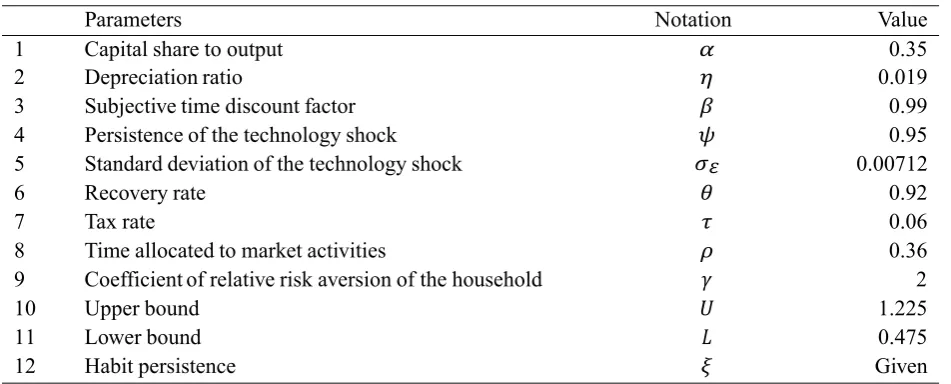
2.2 Calibration

Most values we used for our parameters are standard and borrowed from Alessandrini (2003);

see Table 1. The constant capital share in a Cobb-Douglas production function, , is set to

0.35. The quarterly capital depreciation rate, , is 0.019. The quarterly intertemporal

subjective time discount factor is set to 0.99. The persistence of the idiosyncratic

technology shock, , is given a value of 0.95. The standard deviation of the idiosyncratic

shock is assumed to be 0.00712. The recovery rate, , and tax rate, , are assigned values of

0.92 and 6% respectively.

[Table 1]

We select values for and of 1.225 and 0.475. In the momentary utility function,

we set following Campbell (1994).4 The coefficient of relative risk aversion for the

representative investor’s utility function, , is set to 2. The habit persistence level, , ranges

from 0 to 0.8.

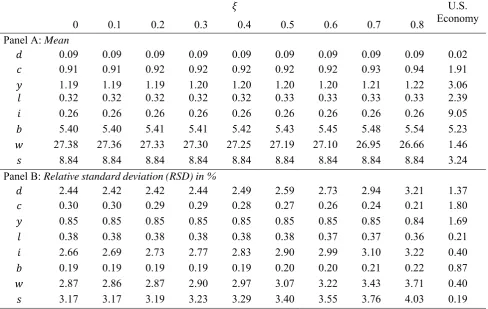
2.3 Results

Our results for the value-maximizing economy are reported in Tables 2 and 3. The former

presents a summary of the mean and the relative standard deviations (RSD) of each

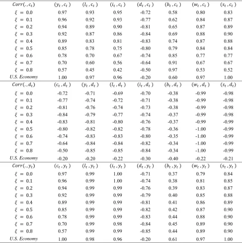
macroeconomic variable.5 The latter presents the correlation of different macroeconomic

variables with consumption, dividend and output.

[Table 2]

[Table 3]

4_{Campbell (1994) sets a value of labor as 0.33 and then obtains the value of the fraction of time devoted to} market activities. Our model shows a steady state value of labor as 0.32 ( ) and 0.33 ( ).

5

Relative standard deviation is each variable’s standard deviations divided by its mean value. It is also known as the ‘coefficient of variation’.

(13)

Panel A of Table 2 shows the estimated steady-state first moment of each variable.

This simulation confirms that the no-trend optimal aggregate dividends are positive and

insensitive to the level of habit persistence ( ). The ratio of the aggregate dividends to salary

( ) is 0.0102 ( meaning that investors get 99% of their income from salary

and 1% from dividends. The aggregate dividends—consumption ratio ( ) is 0.0989

( implying that dividends contribute 10% of investors’ consumption. It is also

worth noting that the consumption—salary ratio ) is 0.1029 ( , indicating

ten per cent of salary goes to investors’ consumption.

As the level of habit persistence ( ) increases from 0 to 0.8, the RSD of aggregate

consumption in Panel B of Table 2 declines from 0.30 to 0.21. That consumption growth

becomes smoother with increased habit motive is consistent with previous research (see, e.g.,

Constantinides, 1990) and this is the central feature that we capture by incorporating habit

formation utility into our economy. In addition, the pro-cyclicality of consumption,

reported in Table 3, becomes less pronounced as the habit motive increases.

How is this consumption smoothing brought about? Consumption comes from three

sources; salary, dividend payments and changes in holding of the risk-free asset after interest

has been paid. Salaries, which are positively correlated with output in all cases because both

the wage rate rises ( ) and people work longer hours ( ) in

benign economic conditions, become both more volatile and more pro-cyclical as the habit

motive gets stronger. As increases from 0 to 0.8, the relative standard deviation of

increases from 3.17 to 4.03 while rises from 0.84 to 0.90. Therefore, somewhat

counter-intuitively, salary effects magnify both the volatility and pro-cyclicality of

consumption growth as the habit motive increases. The observed increased level of

consumption smoothing with higher must then be driven instead by cash flows associated

with financial assets. Consistent with this, bond holding is pro-cyclical in all cases, so

consumption is smoothed to some extent by increasing (decreasing) lending in good (bad)

economic conditions. As increases from 0 to 0.8, rises from 0.37 to 0.44 and

the relative standard deviation of bond holdings increases from 0.19 to 0.22. This does

reduce the volatility and pro-cyclicality of consumption as expected.

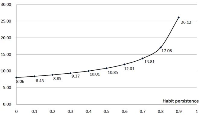
In addition, optimal dividend behavior is highly sensitive to the assumed level of habit

formation. As increases from 0 to 0.8, so the RSD of dividends increases from 2.44 to 3.21

and the payments become more counter-cyclical; increases in absolute terms

(14)

representative agent to smooth consumption. This is further illustrated by Fig. 1, where the

ratio for values of is plotted.

[Figure 1]

This figure shows that, in aggregate, the relative standard deviation of dividends to

consumption rises dramatically as the habit motive becomes large. Counter-cyclical

dividends are offsetting pro-cyclical salary to reduce the consumption volatility of the

representative investor.

An alternate way of illustrating this effect is by examining the correlations of

consumption with its three individual sources. In all cases, consumption is positively

correlated with salary but negatively correlated with the cash flows from risk-free investment

and the equity market.6 However, as the habit motive becomes more intense, the strong

positive relation with salary becomes noticeably weaker. By reducing the reliance of

consumption on salary, dividends help reduce both consumption’s volatility and

pro-cyclicality.

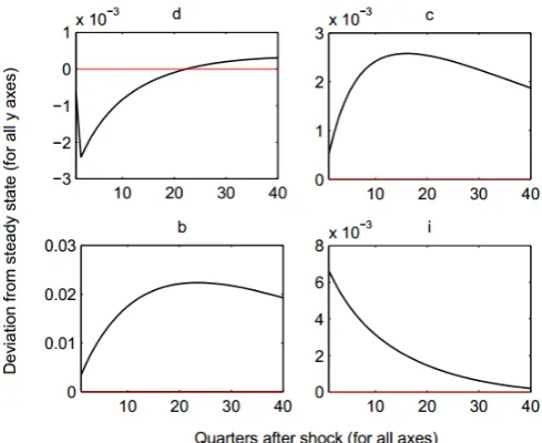
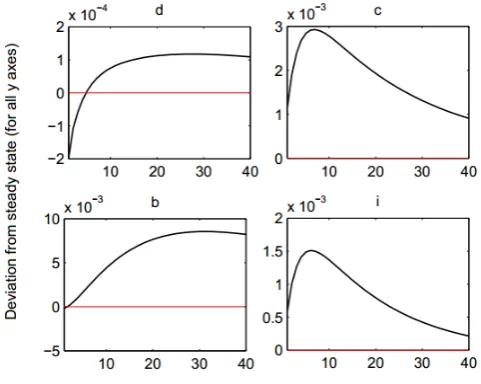
Figs 2 and 3 respectively illustrate the impulse responses of the expected future path

of aggregate dividends and consumption in two cases, without habit formation ) and

with strong habit formation ( ). These response functions further indicate that

consumption growth is smoother when habit persistence is higher. Consumption with the

highest habit motive of has low deviations (far below 0.001) in the first few quarters

after the shock. This contrasts with the no-habit motive case, , when the deviation is

higher than 0.002. The figures further show that aggregate dividends fluctuate more in the

habit formation case than in the no-habit formation case. Notice, for example, that the first

ten quarters’ deviation from the steady state after the shock is between x and

x for the no-habit-motive-investor economy, yet is higher than x for the

with-high-habit-motive-investor economy.

[Figure 2]

[Figure 3]

Aggregate investment, , has similar characteristics to both with and without habit,

in terms of its volatility and the absolute levels of its correlations with consumption and

income. In particular, the optimal investment path becomes more volatile as the habit motive

6_{Remember that is the level of bank lending. So, if}

(15)

increases and investment volatility is close to aggregate payout volatility in each of the

different habit persistence cases. As investors’ habit motive gets stronger, firms must adapt

their own investment plans to ensure that they help maximize the expected utility of the agent.

The correlation between investment and consumption also decreases as the latter is smoothed,

which is consistent with the absolute relationship between dividends and consumption.

Investment is nearly perfectly correlated with output for all values of because of the high

persistence of technology change; . High output this year signals high future

profitability, giving firms a strong incentive to increase investment levels.

In this general equilibrium setting, the habit motive of investors is shown to have a

significant influence not only on investors’ labor and consumption decisions but also on the

investment, financing and payout policy of the firm. This suggests that there is a significant

interaction between corporate policy and investor utility. However, there is one implication

of this model that appears to be at odds with the observed empirical data. In this baseline case,

dividends are predicted to be highly counter-cyclical in each calibration. As we discussed in

the introduction, this is a feature common of many DSGE studies and makes dividends a

highly suitable control variable for smoothing investor consumption across the business cycle.

However, this finding is inconsistent with observed cyclicality of both gross and net

aggregate payout behavior.

To overcome this anomaly, we follow an approach employed by both

Carceles-Poveda (2009) and Huang-Meier et al. (2015), which is to introduce agency conflicts into the

model. This has similar implications for dividend behavior to economies with capital

adjustment costs, but Huang-Meier et al. (2015) argue that agency models better explain

observed market behavior. The results in these studies are also qualitatively comparable to

those of Jermann and Quadrini (2012) who have suggested a relatively complex DSGE model

with both frictions and shocks.

3 Risk-averse firms (RA)

Following Radner (1970), Sandmo (1971) and Leland (1972), in this section we assume that

the firms’ managers maximize their own utility function rather than working in their

shareholders’ best interests. In this risk-averse firms model (RA), managers have risk-averse

(16)

where is the coefficient of relative risk aversion of the manager and denotes the

manager’s time discount factor. Carceles-Poveda (2005, 2009) contend that this risk-aversion

assumption improves our understanding of managers’ behavior. Huang-Meier et al. (2015)

also show that such models significantly change the optimal correlation between dividends

and output. We extend their findings here to a mixed equity and debt environment in the

presence of habit formation.

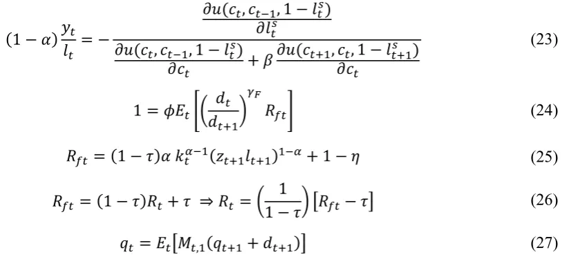
We show in Appendix 3 that solving the household and the firm’s optimization

problem (eqs (2) and (31)) gives a set of five equilibrium conditions for the RA case:

In equilibrium, the above eqs (23) to (27) must hold together with the bank sector (eqs (10)

and (16)) and market clearing conditions ( , , , and ).

To calibrate the RA model, we set equal to 0.99 and equal to 1.44, where these

[image:16.595.109.521.302.496.2]

choices follow Carceles-Poveda (2003). Other parameters remain the same as reported in

Table 1.

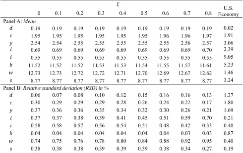
Table 4 displays the results of the mean in Panel A and the RSD in Panel B for each

variable. We notice that the ratio of the positive optimal aggregated dividends to salary ( )

is slightly higher in the RA model than in the VM model. The figure 0.0217 (

implies that agency conflicts bring more dividends to investors’ income. This result is

broadly consistent with the Jensen free cash-flow hypothesis that firms will hold lower levels

of cash in the presence of agency conflicts. The no-trend optimal aggregated dividends to

consumption ratio in the RA model is similar to the VM model while the variances of optimal

max (22)

(23)

(24)

(25)

(26)

(17)

aggregated dividends and consumption are highly sensitive to the level of the habit

persistence. With the exception of consumption and output, the relative volatility of all

variables is substantially lower for the RA model than the VM model. The effect of agency

conflicts leads to a substantial reduction in the volatility of dividend payments, labor hours,

investment, debt financing, the wage rate and salary. For example, the RSD of dividends

with is 2.44 in the VM model but only 0.06 in the RA model.

[Table 4]

Despite this, the RA model provides conclusions that are consistent with our VM

results in that the greater the habit motive the smoother the consumption and the more

volatile the dividend payouts. The RSD of dividend payments more than doubles from 0.06

for to 0.13 for , while consumption volatility almost halves over the same habit

motive interval from 0.30 to 0.17. This again indicates that the aggregate optimal payout

policy is highly sensitive to investor preferences, which is our central finding.

While dividends and consumption respond in similar ways to the changes in the habit

motive in both the VM and RA models, this is not true for many of the other variables under

consideration. Investment, for example, becomes smoother with increased in the RA model,

contrasting with the corresponding result in the VM model. When the habit motive increases

labor hours become more volatile in the RA model, while in the VM model the RSD of labor

hours is largely insensitive to the habit motive. Although the variation of the wage rate

increases with stronger habit motive in both models, our results show that the representative

household’s salary becomes smoother in the RA model while it gets more volatile in the VM

model.

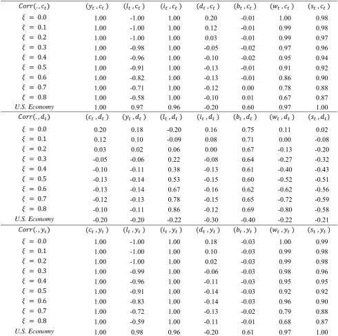
Table 5 presents the cyclicality results for the RA model. Consistent with the findings

of Carceles-Poveda (2009) and Huang-Meier et al. (2015), optimal dividend policy is much

less counter-cyclical in the RA case than the VM case. The values of are in all

cases close to the range of -0.33 to +0.54 reported by Covas and Den Haan (2011), although

remain somewhat less pro-cyclical than suggested by Jermann and Quadrini (2012).

[Table 5]

Consistent with the VM model, dividends become more counter-cyclical as the habit

motive increases; or, more precisely in this case, change from being pro-cyclical for

to counter-cyclical for . Interestingly the effect is non-monotonic for the RA model,

(18)

importantly, our central finding that optimal aggregate dividend policy is highly sensitive to

investor preferences is maintained for the RA case.

There are some other notable differences between the RA and VM models. In the RA

case, consumption remains perfectly correlated with output for all values of considered. So,

while consumption becomes less volatile, it does not become less pro-cyclical in the RA case,

which contrasts with the value maximizing model. Labor hours, which are always highly

pro-cyclical in the VM case, are always highly counter-cyclical in the RA case. This implies

that the representative investor takes some of the benefits from positive technological shocks

through reduced working hours. Despite this, salary remains highly pro-cyclical because of

the increases in wages that results from better technology. In the RA (VM) model, labor

hours becomes less counter-cyclical (the cyclicality is largely unchanged) while the wage rate

becomes less (more) pro-cyclical as the habit motive increases. This leads to salaries

becoming marginally less (marginally more) pro-cyclical as increases.

The other key difference between the RA and VM models concerns the cyclicality of

debt financing. In the RA model, debt is almost uncorrelated with output, while in the VM

model debt is strongly pro-cyclical for all values of considered. It is the VM model that is

more consistent with findings on the cyclicality of corporate debt reported by both Covas and

Den Haan (2011) and Jermann and Quadrini (2012). Therefore there is no strong reason to

prefer either the VM or RA model over the other, but both give similar conclusions for the

importance of aggregate dividends in maximizing investor welfare.

Additionally, we calculate the partial derivatives of optimal aggregated dividends

with respect to the capital share to output, consumption, labor, equity price and technology

shock for both the VM and RA models in the case when the habit persistence equals 0.8. We

document the method and results in Appendix 4. The results of the VM model indicate that

consumption, capital input and labor working hours are negatively related to the optimal

aggregated dividends while the share price and technology shock are positively related to the

optimal aggregated dividends. In order to maintain smooth consumption across time, the

optimal aggregated dividends decrease to balance the investor’s overall income. Unlike the

VM model, the RA model implies a positive partial derivative between consumption and the

optimal aggregated dividends. In the RA model, the household’s consumption is positively

related to labor.

From Figs 4 and 5, we notice that aggregate dividends respond to technology shocks

(19)

as an unexpected bump after the shock and then smooths over a ten quarter interval.

Moreover, optimal consumption in the cases with and without habit motive has distinct

impulse responses to technology shocks. This phenomenon is also found in optimal

investment.

[Figure 4]

[Figure 5]

4 The US economy: the cyclical volatility correlation

This section compares the implications of our models to several key features observed in the

US economy over the period 1964Q2 to 2010Q1. Specifically, we follow Jermann and

Quadrini (2012) and collect quarterly financial data series from the Flow of Funds Accounts

of the Federal Reserve Board (FFA) and economic data from National Income and Product

Accounts (NIPA), the Bureau of Labor Statistics (BLS), and the Current Employment

Statistics (CES).

A detailed definition for each series is: Equity payouts proxy for dividends (d) and are

the sum of net dividends of nonfarm, nonfinancial and farm business (FFA codes

FA106121075 and Z1/OTHER/FA136121073), minus the total of net increases in corporate

nonfinancial business and proprietors net investment in nonfinancial business (FFA codes

FA103164103 and FA112090205); Consumption (c) is defined as real personal consumption

expenditures (NIPA Table 1.1.6); GDP (y) is the total of real gross domestic product, from

U.S. Department of Commerce: Bureau of Economic Analysis; Labor income represents

salary (s) and is defined as wages times working hours. We use the data for real hourly

compensation in the business sector (from BLS) for wages (w) and total private aggregate

weekly hours (CES, national survey) for labor working hours (l); Capital expenditures are taken from nonfinancial business from FFA Table F.101, line 4 are the measure for

investment (i); Debt (b) is the total liabilities in nonfinancial business (FA144190005). All

series are in billions of dollars and seasonally adjusted. Following Jermann and Quadrini

(2012) we deflate equity payouts, by business value added from NIPA (Table 1.3.5) and

capital expenditures and debt by the price index for business value added from NIPA (Table

1.3.4). We also deflate consumption and GDP in the same manner as equity payouts and we

deflate wages following the procedure for capital expenditures.

We report the mean and RSDs of these empirical series in the final columns of Tables

(20)

our models are broadly consistent with the observed data. Of particular importance for this

paper, both models capture the observed negative correlation between consumption and

dividends except in the case of low values of in the RA model. They also both provide an

explanation of the negative relationship between dividend and salary payments.

The different models explain different features of the observed data. The RA model

with =0.3 captures many of the characteristics of the observed correlations and is, perhaps,

the best fitting model. This accurately represents the negative correlation between salary

payments and dividends. However, it cannot explain the behavior of either labor hours or

debt. As a consequence, as with other models, it also overestimates the importance of wages

as a source of income. More generally, the RA model does better than the VM model in

capturing the variation of investment and the average levels of consumption and output. By

contrast, the VM model captures well the mean values of equity payouts and debt. In

addition, our VM model estimates that the correlation between dividends and debt, Corr(b,d),

lies within the range -0.34 and -0.38, which is close to the figure of -0.40 for the empirical

series. It also more accurately captures the observed values of Corr(l,c) and Corr(b,c)

compared to the RA model.

Therefore, although neither model can fully capture all features of the observed

economy, their implications are largely consistent with observed phenomenon. The

relationship between dividends and consumption predicted by the RA model with moderate

values of habit formation accurately reflects the real-world behavior that is the specific focus

of this study.

5 Conclusions

In this paper, we study business cyclical behaviors of aggregate activities by looking at the

effect of investors’ preference. We demonstrate that dividends play a vital role in helping to

isolate investors from the volatility of the business cycle both in the absence and presence of

agency conflicts. In particular, we show that optimal dividend payout policy has increasing

relative standard deviation and becomes more negatively correlated with output as the habit

motive increases. This volatile and counter-cyclical stream of financial income helps

counterbalance the highly pro-cyclical nature of salaries in economies when the habit motive

is strong.

Using a macroeconomic dynamic stochastic general equilibrium approach to study the

(21)

theoretical framework to support the conjecture by Marsh and Merton (1987) that aggregate

dividend policy remains relevant even when investors are less concerned about which

individual firm services this demand for equity income. Our study sheds light on the

relationship between aggregate dividend policy and investor utility; an issue that has rarely

been previously discussed in the standard corporate finance literature. We believe that this

opens a large number of areas for future research. This work could be extended, for example,

by examining optimal aggregate dividend and investment policy in an economy with

irreversible investment.

A further important potential extension would be to apply generalized method of

moments (GMM) methods to estimate and test the moment conditions of this framework.

This would follow in the path of a number of empirical studies, including Yogo (2006), who

applies GMM to test the moment conditions of models that use durable consumption to

explain expected stock returns. Darrat et al. (2011) also use GMM to estimate and test their

model that provides evidence of the existence of idiosyncratic consumption risk sharing

across countries, while Savov (2011) implements a similar approach to test a

consumption-based capital asset pricing model that introduces garbage growth as a measure of

consumption growth. Verifying the robustness of our findings to these additional tests would

provide further support to our conclusion that aggregate dividends play a vital role in helping

investors optimally smooth their consumption paths.

References

Alessandrini, F. (2003) Introducing capital structure in a production economy: Implications for investment, debt and dividends, available at https://ideas.repec.org/p/lau/crdeep/03.03.html.

Allen, F. and Michaely, R. (2003) Payout policy, in G.M. Constantinides, M. Harris, and R.M. Stulz (eds), Handbook of the Economics of Finance, Elsevier, North Holland.

Bansal, R. and Yaron, A. (2004) Risks for the long run: a potential resolution of asset pricing puzzles, Journal of Finance, 59, 1481–509.

Baxter, M., Jermann, U., and King, R. (1998) Nontraded goods, nontraded factors, and international non-diversification, Journal of International Economics, 44, 211–29.

Ben-David, I. (2010) Dividend policy decisions, in H.K. Baker and J.R. Nofsinger (eds), Behavioral Finance: Investors, Corporations, and Markets, John Wiley & Sons.

Benartzi, S., Michaely, R., and Thaler, R. (1997) Do changes in dividends signal the future or the past?, Journal of Finance, 52, 1007–34.

(22)

fallacy, Bell Journal of Economics, 10, 259–70.

Boldrin, M., Christiano, L., and Fisher, J. (2001) Habit persistence, asset returns, and the business cycle, American Economic Review, 91, 149–66.

Brav, A., Graham, J., Harvey, C., and Michaely, R. (2005) Payout policy in the 21st century, Journal of Financial Economics, 77, 483–527.

Brennan, M. (1970) Taxes, market valuation and corporate financial policy, National Tax Journal, 23, 417–27.

Campbell, J. (1994) Inspecting the mechanism: an analytical approach to the stochastic growth model, Journal of Monetary Economics, 33, 463–506.

Campbell, J.Y. and Cochrane, J.H. (1999) By force of habit: a consumption-based

explanation of aggregate stock market behavior, Journal of Political Economy, 107, 205–

51.

Carceles-Poveda, E. (2003) Capital adjustment costs and firm risk aversion, Economics Letters, 81, 101–7.

Carceles-Poveda, E. (2005) Idiosyncratic shocks and asset returns in the real-business-cycle model: an approximate analytical approach, Macroeconomic Dynamics, 9, 295–320.

Carceles-Poveda, E. (2009) Asset prices and business cycles under market incompleteness, Review of Economic Dynamics, 12, 405–22.

Carroll, C., Overland, J., and Weil, D. (2000) Saving and growth with habit formation, American Economic Review, 90, 341–55.

Constantinides, G. (1990) Habit formation: a resolution of the equity premium puzzle, Journal of Political Economy, 98, 519–43.

Covas, F. and Den Haan, W. (2011) The cyclical behavior of debt and equity finance, American Economic Review, 101, 877–99.

Darrat, A.F., Li, B., and Park, J.C. (2011) Consumption-based CAPM models: international evidence, Journal of Banking & Finance, 35, 2148–57.

DeAngelo, H., DeAngelo, L., and Skinner, D. (1996) Reversal of fortune dividend signaling and the disappearance of sustained earnings growth, Journal of Financial Economics, 40, 341–71.

Dennis, R. (2009) Consumption habits in a new Keynesian business cycle model, Journal of Money, Credit and Banking, 41, 1015–30.

Dong, M., Robinson, C., and Veld, C. (2005) Why individual investors want dividends, Journal of Corporate Finance, 12, 121–58.

Easterbrook, F. (1984) Two agency-cost explanations of dividends, American Economic Review, 74, 650–9.

Fuhrer, J. (2000) Habit formation in consumption and its implications for monetary-policy models, American Economic Review, 90, 367–90.

Fuller, K. and Goldstein, M. (2011) Do dividends matter more in declining markets?, Journal of Corporate Finance, 17, 457–73.

(23)

Financial Economics, 19, 19–27.

Hansen, G. (1985) Indivisible labor and the business cycle, Journal of Monetary Economics,

16, 309–27.

Harris, T., Hubbard, R., and Kemsley, D. (2001) The share price effects of dividend taxes and tax imputation credits, Journal of Public Economics, 79, 569–96.

Hirshleifer, D. A., Li, J., and Yu, J. (2015) Asset pricing in production economies with extrapolative expectations, available at http://dx.doi.org/10.2139/ssrn.1785961.

Huang-Meier, W., Freeman, M. C., and Mazouz, K. (2015) Why are aggregate equity payouts pro-cyclical?, Journal of Macroeconomics, 44, 98–108.

Jensen, M. (1986) Agency costs of free cash flow, corporate finance, and takeovers, American Economic Review, 76, 323–9.

Jensen, M. and Meckling, W. (1976) Theory of the firm: managerial behavior, agency costs, and Capital Structure, Journal of Financial Economics, 3, 305–60.

Jermann, U. and Quadrini, V. (2012) Macroeconomic effects of financial shocks, American Economic Review, 102, 238–71.

Ju, N. and Miao, J. (2012) Ambiguity, learning, and asset returns, Econometrica, 80, 559– 91.

Kydland, F. and Prescott, E. (1982) Time to build and aggregate fluctuations, Econometrica: Journal of the Econometric Society, 50, 1345–70.

La Porta, R., Lopez-de Silanes, F., Shleifer, A., and Vishny, R. (2000) Agency problems and dividend policies around the world, Journal of Finance, 55, 1–33.

Leland, H. (1972) Theory of the firm facing uncertain demand, American Economic Review,

62, 278–91.

Lettau, M., and Uhlig, H. (2000) Can habit formation be reconciled with business cycle

facts?, Review of Economic Dynamics, 3, 79–99.

Levy, A. and Hennessy, C. (2007) Why does capital structure choice vary with macroeconomic conditions?, Journal of Monetary Economics, 54, 1545–64.

Liu, H. and Miao, J. (2015) Growth uncertainty, generalized disappointment aversion and production-based asset pricing, Journal of Monetary Economics, 69, 70–89.

Marsh, T. and Merton, R. (1987) Dividend behavior for the aggregate stock market, Journal of Business, 60, 1–40.

Miller, M. H. and Modigliani, F. (1961) Dividend policy, growth, and the valuation of shares, Journal of Business, 34, 411–33.

Miller, M. H. and Rock, K. (1985) Dividend policy under asymmetric information, Journal of Finance, 40, 1031–51.

Miller, M. and Scholes, M. (1978) Dividends and taxes, Journal of Financial Economics, 6, 333–64.

Modigliani, F. and Miller, M. H. (1963) Corporate income taxes and the cost of capital: a correction, American Economic Review, 53, 433–43.

(24)

equity premium puzzle?, Journal of Monetary Economics, 49, 1261–88.

Pettit, R. (1977) Taxes, transactions costs and the clientele effect of dividends, Journal of Financial Economics, 5, 419–36.

Poterba, J. and Summers, L. (1985) The economic effects of dividend taxation, available at http://www.nber.org/papers/w1353.

Radner, R. (1970) Problems in the theory of markets under uncertainty, American Economic Review, 60, 454–60.

Sandmo, A. (1971) On the theory of the competitive firm under price uncertainty, American Economic Review, 61, 65–73.

Savov, A. (2011) Asset pricing with garbage, Journal of Finance, 66, 177–201.

Seckin, A. (2001) Consumption–leisure choice with habit formation, Economics Letters, 70, 115–20.

Yogo, M. (2006) A consumption based explanation of expected stock returns, Journal of

(25)

Appendices

Appendix 1: Proof of eqs (17) to (21) (Equilibrium conditions for the economy environment including a representative household and a value-maximizing firm)

First, the representative household’s optimal problem (eq. (2)) is solved by:

subject to the budget constraint (eq. (3))

The Lagrangian of the household’s optimal problem can be written as:

where is a Lagrangian multiplier. Solving for the first-order conditions yields:

Substituting the Lagrangian multiplier from eq. (A.2) into eq. (A.3), the wage rate for

labor in supply is:

Eq. (A.4) leads a standard Euler equation for the price of equity:

max

(A.1)

(A.2)

(A.3)

(A.4)

(A.5)

(A.6)

(26)

where is defined as the intertemporal marginal rate of substitution with respect to consumption.

Rewriting eq. (A.5) with , we obtain the the standard Euler equation:

So that the above eqs (A.6), (A.7), and (A.8) are the household’s optimal first order conditions.

Next, we solve the representative firm’s optimal problem (eq. (14)):

subject to the constraints of the capital function (eq. (7)) and dividends to shareholders (eq.

(9)):

The Lagrangian of the firm’s optimization problem can be written as:

Differentiating eq. (A.10) with respect to , and and setting the values each time to zero yields:

(A.8)

max

(A.9)

(A.10)

(A.11)

(A.12)

(27)

Using eqs (A.6) to (A.8) and (A.11) to (A.13), we can derive the value-maximizing model’s equilibrium conditions. Specifically, using eqs (A.6) and (A.11), the optimal wage rate for labor takes the following form:

Using eqs (A.8) and (A.12), we get:

Using eqs (A.8) and (A.13), the relationship between the risk-free interest rate and the corporate interest rate is:

For the price of equity, we rewrite eq. (A.7) here:

So that eqs (A.14) to (A.18) are the equilibrium conditions eqs (17) to (21) shown in Section 2.1.5. We show a specific form of in Appendix 2.

Appendix 2: The intertemporal marginal rate of substitution with consumption,

In eq. (A.7), we define the intertemporal marginal rate of substitution in the following form:

From eq. (A.2), we know that:

Substituting eqs (A.20) and (A.21) into eq. (A.19):

(A.14)

(A.15)

(A.16)

(A.17)

(A.18)

(A.19)

(A.20)

(A.21)

(28)

Next, we apply the household’s momentary utility function to eq. (A.22). We assume that

household utility is determined by the multiplied effect of consumption and leisure, which

can be written as:

With the given momentary utility function, we calculate , , ,

, , and :

Finally, the intertemporal marginal rate of substitution with consumption can be written as:

Appendix 3: Proof of eqs (23) to (27) (Equilibrium conditions for the economy environment including a representative household and a risk-averse firm)

This appendix obtains equilibrium conditions when the firm no longer maximizes shareholders’ value but instead possesses its own risk aversion characteristic.

The household’s maximization preference does not change and therefore the first order conditions for the household’s problem remain the same as in the case of the value-maximization model as given in eqs (A.6), (A.7), and (A.8).

To solve the risk-averse firm’s problem (eq. (22)):

(A.23)

(A.24)

(A.25)

(A.26)

(A.27)

(A.28)

(A.29)

(A.30)

(29)

subject to the constraint of dividends to shareholders (eq. (9), where is replaced by eq. (7)):

Setting the partial derivatives of the firm’s objective function with respect to , , and all

equal to zero, the first order conditions for the firm’s problem are:

The above eqs (A.34) to (A.36) are the risk-averse firm’s optimal conditions.

The next step is to tidy up the six first order conditions (eqs (A.6) to (A.8) and (A.34) to (A.36)). From eqs (A.6) and (A.34), we know that the optimal wage rate for labor takes the following form:

From eqs (A.8) and (A.35):

where can be regarded as being the equivalent to from the value-maximizing

model.

Using eqs (A.8) and (A.36), we can obtain the relationship between the risk-free interest rate and the corporate interest rate in the absence of bankruptcy:

For the price of equity, we repeat eq. (A.7) here:

max (A.32)

(A.33)

(A.34)

(A.35)

(A.36)

(A.37)

(A.38)

(A.39)

(A.40)

(30)

So that eqs (A.37) to (A.41) are the equilibrium conditions eqs (23) to (27) shown in Section 3. The variable includes the household’s utility function with habit formation; refer to Appendix 2 for details.

Appendix 4: The partial derivatives of dividends with respect to explanatory variables

Consider the optimal aggregated dividend as a linear function of underlying variables:

To derive the partial derivative of dividends with respect to each variable, we first construct a 5-vector of the covariance of each explanatory variable with ; . We also construct a variance-covariance matrix of all explanatory variables, , with the ith row given by , and a 5-vector, with elements that denote the partial derivatives:

We calculate the partial derivative of the optimal aggregated dividends with respect to capital input ( ), consumption (c), labor (l), equity price (q) and technology shock (z) for the VM model and the RA model in the case of habit persistence of 0.8:

(31)

[image:31.595.112.442.86.279.2]

(32)

[image:32.595.176.420.88.294.2]

Fig. 2. The impulse responses of optimal aggregate dividends ( ), consumption ( ), debt ( ), and investment ( ) in the case without habit persistence for the VM model ( )

[image:32.595.174.419.377.577.2]

(33)

[image:33.595.185.437.68.264.2]

Fig. 4. The impulse responses of optimal aggregate dividends ( ), consumption ( ), debt ( ), and investment ( ) in the case without habit persistence for the RA model ( )

[image:33.595.193.434.355.547.2]

(34)

[image:34.595.71.547.87.279.2]

Table 1. Calibration values for the models’ parameters

Parameters Notation Value

1 Capital share to output 0.35

2 Depreciation ratio 0.019

3 Subjective time discount factor 0.99

4 Persistence of the technology shock 0.95

5 Standard deviation of the technology shock 0.00712

6 Recovery rate 0.92

7 Tax rate 0.06

8 Time allocated to market activities 0.36

9 Coefficient of relative risk aversion of the household 2

10 Upper bound 1.225

11 Lower bound 0.475

12 Habit persistence Given

(35)

[image:35.595.74.563.107.416.2]

Table 2. Mean and relative standard deviation (RSD in %) for the VM model and the US economy

U.S. Economy

0 0.1 0.2 0.3 0.4 0.5 0.6 0.7 0.8

Panel A: Mean

0.09 0.09 0.09 0.09 0.09 0.09 0.09 0.09 0.09 0.02

0.91 0.91 0.92 0.92 0.92 0.92 0.92 0.93 0.94 1.91

1.19 1.19 1.19 1.20 1.20 1.20 1.20 1.21 1.22 3.06

0.32 0.32 0.32 0.32 0.32 0.33 0.33 0.33 0.33 2.39

0.26 0.26 0.26 0.26 0.26 0.26 0.26 0.26 0.26 9.05

5.40 5.40 5.41 5.41 5.42 5.43 5.45 5.48 5.54 5.23

27.38 27.36 27.33 27.30 27.25 27.19 27.10 26.95 26.66 1.46

8.84 8.84 8.84 8.84 8.84 8.84 8.84 8.84 8.84 3.24

Panel B: Relative standard deviation (RSD) in %

2.44 2.42 2.42 2.44 2.49 2.59 2.73 2.94 3.21 1.37

0.30 0.30 0.29 0.29 0.28 0.27 0.26 0.24 0.21 1.80

0.85 0.85 0.85 0.85 0.85 0.85 0.85 0.85 0.84 1.69

0.38 0.38 0.38 0.38 0.38 0.38 0.37 0.37 0.36 0.21

2.66 2.69 2.73 2.77 2.83 2.90 2.99 3.10 3.22 0.40

0.19 0.19 0.19 0.19 0.19 0.20 0.20 0.21 0.22 0.87

2.87 2.86 2.87 2.90 2.97 3.07 3.22 3.43 3.71 0.40

3.17 3.17 3.19 3.23 3.29 3.40 3.55 3.76 4.03 0.19

(36)

[image:36.595.59.547.86.575.2]

Table 3. Cross-correlations of real variables (VM model and the US economy)

c

0.97 0.93 0.95 -0.72 0.58 0.80 0.83

0.96 0.92 0.93 -0.77 0.62 0.84 0.87

0.94 0.89 0.90 -0.81 0.65 0.87 0.89

0.92 0.87 0.86 -0.84 0.69 0.88 0.90

0.89 0.83 0.81 -0.83 0.74 0.87 0.88

0.85 0.78 0.75 -0.80 0.79 0.84 0.84

0.78 0.70 0.67 -0.74 0.85 0.77 0.77

0.70 0.60 0.56 -0.64 0.91 0.67 0.67

0.57 0.45 0.42 -0.50 0.97 0.53 0.52

U.S. Economy 1.00 0.97 0.96 -0.20 0.60 0.97 1.00

-0.72 -0.71 -0.69 -0.70 -0.38 -0.99 -0.98

-0.77 -0.74 -0.72 -0.71 -0.38 -0.99 -0.98

-0.81 -0.76 -0.74 -0.73 -0.38 -0.99 -0.98

-0.84 -0.79 -0.77 -0.74 -0.37 -0.99 -0.98

-0.83 -0.81 -0.80 -0.76 -0.37 -0.99 -0.99

-0.80 -0.82 -0.82 -0.78 -0.36 -1.00 -0.99

-0.74 -0.83 -0.83 -0.80 -0.35 -1.00 -0.99

-0.64 -0.84 -0.84 -0.82 -0.34 -1.00 -0.99

-0.50 -0.85 -0.85 -0.84 -0.34 -1.00 -0.99

U.S. Economy -0.20 -0.20 -0.22 -0.30 -0.40 -0.22 -0.21

0.97 0.99 1.00 -0.71 0.37 0.79 0.84

0.96 0.99 1.00 -0.74 0.38 0.81 0.85

0.94 0.99 0.99 -0.76 0.39 0.83 0.87

0.92 0.99 0.99 -0.79 0.40 0.85 0.88

0.89 0.99 0.99 -0.81 0.41 0.86 0.89

0.85 0.99 0.99 -0.82 0.42 0.87 0.90

0.78 0.99 0.99 -0.83 0.44 0.88 0.90

0.70 0.99 0.98 -0.84 0.45 0.89 0.90

0.57 0.99 0.99 -0.85 0.44 0.89 0.90

U.S. Economy 1.00 0.98 0.96 -0.20 0.61 0.97 1.00

(37)

[image:37.595.71.562.89.399.2]

Table 4. Mean and relative standard deviation (RSD in %) for the RA model

U.S. Economy

0 0.1 0.2 0.3 0.4 0.5 0.6 0.7 0.8

Panel A: Mean

0.19 0.19 0.19 0.19 0.19 0.19 0.19 0.19 0.19 0.02 1.95 1.95 1.95 1.95 1.95 1.95 1.96 1.96 1.97 1.91 2.54 2.54 2.55 2.55 2.55 2.55 2.55 2.56 2.57 3.06 0.69 0.69 0.69 0.69 0.69 0.69 0.69 0.69 0.70 2.39 0.55 0.55 0.55 0.55 0.55 0.55 0.55 0.55 0.55 9.05 11.52 11.52 11.52 11.53 11.53 11.54 11.55 11.57 11.61 5.23 12.73 12.73 12.72 12.72 12.71 12.70 12.69 12.67 12.62 1.46 8.77 8.77 8.77 8.77 8.77 8.77 8.77 8.77 8.77 3.24 Panel B: Relative standard deviation (RSD) in %

0.06 0.07 0.08 0.10 0.12 0.15 0.16 0.16 0.13 1.37

0.30 0.29 0.29 0.29 0.28 0.26 0.24 0.22 0.17 1.80

0.37 0.36 0.36 0.35 0.34 0.32 0.30 0.26 0.21 1.69

0.37 0.37 0.38 0.39 0.41 0.45 0.51 0.59 0.70 0.21

0.58 0.58 0.57 0.56 0.54 0.51 0.48 0.42 0.33 0.40

0.04 0.04 0.04 0.04 0.04 0.04 0.04 0.03 0.03 0.87

0.74 0.75 0.76 0.78 0.80 0.84 0.88 0.92 0.95 0.40

0.38 0.38 0.38 0.39 0.39 0.39 0.38 0.34 0.27 0.19

(38)

[image:38.595.57.548.83.569.2]

Table 5. Cross-correlations of real variables (RA model)

c