First-order turbulence closure for modelling complex canopy flows

This is a repository copy of First-order turbulence closure for modelling complex canopy flows.

White Rose Research Online URL for this paper: http://eprints.whiterose.ac.uk/85707/

Version: Accepted Version

Article:

Finnigan, J, Harman, I, Ross, AN et al. (1 more author) (2015) First-order turbulence closure for modelling complex canopy flows. Quarterly Journal of the Royal Meteorological Society, 141 (692). pp. 2907-2916. ISSN 0035-9009

https://doi.org/10.1002/qj.2577

eprints@whiterose.ac.uk Reuse

Unless indicated otherwise, fulltext items are protected by copyright with all rights reserved. The copyright exception in section 29 of the Copyright, Designs and Patents Act 1988 allows the making of a single copy solely for the purpose of non-commercial research or private study within the limits of fair dealing. The publisher or other rights-holder may allow further reproduction and re-use of this version - refer to the White Rose Research Online record for this item. Where records identify the publisher as the copyright holder, users can verify any specific terms of use on the publisher’s website.

Takedown

If you consider content in White Rose Research Online to be in breach of UK law, please notify us by

First-order turbulence closure for modelling complex canopy

fl

_ows

John Finnigan1, Ian Harman1, Andrew Ross2 and Stephen Belcher3

1. CSIRO Oceans and Atmosphere Flagship, Canberra Australia 2 School of Earth and Environment, University of Leeds, UK. 3 The Hadley Centre, the Meteorological Office, Exeter, UK.

Submitted in revised form to Quart. Journal of Roy. Meteorol. Soc. 27/3/15

Abstract

Simple first-order closure remains an attractive way of formulating equations for

complex canopy flows when the aim is to find analytic or simple numerical solutions to

illustrate fundamental physical processes. Nevertheless, the limitations of such closures

must be understood if the resulting models are to illuminate rather than mislead. We

propose five conditions that first-order closures must satisfy then test two widely used

closures against them. The first is the eddy diffusivity based on a mixing length. We

discuss the origins of this approach, its use in simple canopy flows and extensions to

more complex flows. We find that it satisfies most of the conditions and, because the

reasons for its failures are well understood, it is a reliable methodology. The second is

the velocity-squared closure that relates shear stress to the square of mean velocity.

Again we discuss the origins of this closure and show that it is based on incorrect

physical principles and fails to satisfy any of the five conditions in complex canopy

flows; consequently its use can lead to actively misleading conclusions.

1. Introduction

At present over 400 FLUXNET Ôeddy-fl_{uxÕ tower sites are operated on a long-term and}

continuous basis in order to infer net exchange of energy, carbon dioxide and other trace

gases between the local ecosystem and the atmosphere (http://fl_{uxnet.ornl.gov). In many}

cases such interpretation is confounded by the impacts of complex terrain on the

atmospheric transport of matter, momentum and energy (Schimel et al., 2008; Finnigan

2008). Flows through fragmented forest canopies are also of great interest in the context

of wind damage while urban canopies with changing building density define the

conditions for urban pollution spread and the wind environment of cities. To understand

rst-2 

order) fl_{ow and transport models that allow analytic solutions or simple numerical}

computations that are not opaque Ôblack boxesÕ (e.g. Belcher et al., 2003; Finnigan and

Belcher, 2004; Yi et al., 2005; Katul et al., 2006; Yi, 2008; Ross, 2012). It is important

that the fl_{uid mechanical principles underpinning such models be sound as the}

community increasingly relies on them for data interpretation. Although modelling is the

primary motivation for this paper it is worth noting that several authors recently have

used mixing lengths to interpret observed canopy flow statistics (eg., Poggi et al., 2004;

Bai et al., 2012). The use of mixing lengths and eddy viscosities in canopy flows was

common before the role of large eddy structure and the consequent absence of local

equilibrium in the canopy turbulent kinetic energy and stress budgets was understood

(Finnigan, 2000) but in fact the use of such concepts is very circumscribed as we shall

show so the development below is also relevant to experimental studies.

Before going further, it is necessary to be more precise about what we mean by simple

and complex canopy flows. All canopy flows are microscopically complex as the flow

threads its way through the foliage airspace but at a macroscopic scale encompassing

many plants, simple canopies are only heterogeneous in the vertical. So by a simple

canopy flow we mean a statistically stationary flow in a horizontally homogeneous

canopy on level ground. Such a flow has only one element in its mean rate-of-strain

tensor: the vertical shear in the mean wind. In contrast, by complex canopy flows we

mean flows in canopies on hills or with rapidly varying foliage area density such as gaps

and clearings or flows that are unsteady on time scales comparable to the integral time

scales of the turbulence. Such flows can exhibit mean strain rates along all three space

axes. In this note we fi_{rst discuss the fundamental requirements that simple} fi_rst-order

closures for models applied to complex canopy fl_{ows must satisfy. Then we review}

whether the closure schemes employed by two groups of models-mixing length closures

eg. Finnigan and Belcher (2004) or Ross (2012) and the velocity-squared closure eg Yi

et al. (2005, 2008)-satisfy these requirements and illustrate how failure to do so can lead

to incorrect results or inferences.

We find that mixing-length-based eddy diffusivity closures satisfy the fundamental

where foliage density changes significantly over length scales shorter than the integral

length scale of the turbulence or where the turbulence is strained rapidly relative to its

integral time scale. In the first case non-local effects degrade the relationship between

local turbulent stress and local rate of mean straining and in the second, viscoelastic

effects introduce ÔmemoryÕ of earlier straining into the turbulent stress response.

Nevertheless, in both cases, the nature of the closure ensures that the turbulent flow is

modelled as a Stokesian fluid so that basic thermodynamic relationships are preserved.

The velocity-squared closure, in contrast, fails to give physically realistic results even in

the simple canopy shear flows for which it was originally derived. In particular, it

predicts that the canopy velocity profile is independent of canopy element drag

coefficient. In more complex flows where both streamwise pressure gradients and shear

stress gradients are combined, we find that the closure inevitably co-locates maxima in

shear stress and maxima in mean velocity whereas in reality, shear stress maxima are

found close to maxima in velocity gradient, independent of the velocity magnitude,

which may be close to zero there. As a result, the closure fails to satisfy the fundamental

criteria and contradicts basic thermodynamic requirements. We conclude that it is

generally unsafe to use this closure in simple models.

2. Turbulence closure in complex canopy flows

The equations that describe fl_{ow in the canopy airspace are derived using a Ôdouble}

averagingÕ technique with successive application of time and spatial averaging to the

Navier Stokes equations (Raupach and Shaw, 1982; Finnigan, 1985; Brunet et al., 1994;

Finnigan and Shaw, 2008). It is now usual to perform the spatial averaging over thin

slabs confi_{ned between coordinate surfaces that follow the ground contour, such as}

surface-following or streamline coordinates. With the assumption that the canopy is

laterally uniform on a scale much larger than the plants, choosing thin slabs as the

averaging volume allows the averaged variables to refl_{ect the characteristic vertical}

heterogeneity of the canopy but to smooth out smaller scale spatial fl_{uctuations caused}

as air fl_{ows around leaves, stems and branches. The resulting time and space-averaged}

4  ∂ _u

i ∂_t + uj

∂ _u i ∂_x

j +

∂ u_i′′u′′_j ∂_x

j +

∂ u′_iu′_j ∂_x

j

=−∂ p ∂_x

i

− ∂ ′′p ∂_x

i

+ν ∂ 2

u_i

∂_x j∂xj

+ν ∂ 2

′′

u_i

∂_x j∂xj

a

∂ u_i

∂_x i

=∂ui ′′ ∂_x

i =∂_∂ui

x_i =

∂_u i′ ∂_x

i

=0 _b

(1)

where we use a right handed Cartesian coordinate system x

i with x₁ in the streamwise

direction and x

3 normal to the ground surface; ui is the corresponding velocity vector, ν is the kinematic viscosity and p the kinematic pressure departure from a hydrostatic

reference state. In equation (1) and in the rest of this paper we ignore diabatic effects in

the flow. The overbar denotes the time average with single primes the instantaneous

departures from that average while angle brackets denote the spatial average with double

primes the local departures from that average. In (1) we have ignored terms

compensating for the volume fraction occupied by solids in the canopy space because

these are negligible in natural vegetation although they must be included in urban

canopies and some wind tunnel models (e.g. Bšhm et al., 2013).

Just as in the conventional Reynolds equations for time or ensemble averaged velocity,

in solving or modelling (1) we confront a closure problem because, even after using

continuity (1)b to eliminate the pressure, equation (1)a contains terms that cannot be

expressed as functions of u

i without further assumptions. The two such terms on the right hand side of (1)a can be shown to correspond to F_{Di, the aerodynamic drag exerted}

by the canopy on the air in the averaging volume. It is usual in the high Reynolds

number conditions of natural canopies to parameterise the total aerodynamic drag as if it

were all exerted by pressure forces and so proportional to the square of the windspeed

past the canopy elements; hence we write,

F_Di =− ∂p ′′

∂_x i

+υ ∂

2_u

i ′′

∂_x j

2 =−cda u

(

i−vi

)

ui−vi (2)

where c_{dis a dimensionless drag coefficient, a is the foliage area per unit volume of}

space and v

i is the canopy element velocity. It is apparent, however that equation (2) as

u_i−v_i

(

)

u_i−v_{i contains a mixture of mean and turbulent velocity fluctuations. As a}

result, the parameterization (2) is usually simplified to,

F_{Di =−}c_da

(

u_i−v_i

)

(

u_i−v_i

)

     ₍₃₎ 

which ensures that the drag force is a vector proportional to the square of the wind

velocity relative to the foliage and always directed against the wind.

The inclusion of the element velocity,v

i in (3) serves two purposes. First, it allows us to

deal with flexible canopies that wave in the wind. Although in most practical examples

flexibility effects can be neglected, they can be important in the case of coherently

waving canopies (de Langre, 2008; Dupont et al., 2010; Finnigan, 1985; Finnigan,

2010). Second, it satisfies the requirement that the parameterized equation be Galilean

invariant, that is, that the equation remain physically correct if the axes are translated

with constant velocity. For the case of axes fixed in space and rigid canopy elements,

v

i=0 and for simplicity, in the rest of this paper, we will assume this to be the case.

Comparing equations (2) and (3) we see that parameterization (3) leaves some residual

dependence on turbulent intensity and scale in the drag coefficient c_{d as well as on}

canopy element Reynolds number because at lower wind speeds the viscous term, which

varies as u i 3/2

, can make a signifi_{cant contribution to the drag. These points are}

discussed at length in Brunet et al. (1994).

The terms on the left hand side of (1) that require closure assumptions are the fi_{rst two}

terms in the expression for the total kinematic stress tensor,

σ

ij =− ui′′u′′j − ui′u′j +ν

∂ u_i ∂x_j +

∂ u_j ∂x_i ⎡

⎣ ⎢ ⎢

⎤

⎦ ⎥

⎥− p δij (4)

where δ

ij is the Kronecker delta and we have followed standard manipulations (eg.

Hinze, 1975) and written the mean viscous stress as the product of the kinematic

viscosity and the mean rate of strain tensor, to ensure invariance under exchange of

6 

as the Reynolds stresses, u_i′u_j′ do to time averaging but are almost always, when

modelling, added to the Reynolds stresses to form the total ÔturbulentÕ stress. For a

fuller discussion see Finnigan (1985) and Finnigan and Shaw (2008). In what follows,

for simplicity we combine Reynolds and dispersive stresses as the total turbulent stress,

σ

ij t

=− _u′′_iu′′_j − _ui′_u′_j (5)

In atmospheric flows the mean viscous stress, ν ∂⎡⎣ ui ∂xj+∂ uj ∂xi⎤⎦ is two or three

orders of orders of magnitude smaller than the other terms in (4) and so is usually

neglected.

It is useful at this point to outline a set of requirements that any closure for the turbulent

stress needs to satisfy to be applicable to canopy fl_{ows in complex terrain. These}

fundamental requirements are essentially the same as those that apply to higher order

closures as set out in detail in Lumley (1978), namely that the closure must be:

I. coordinate invariant and material frame indifferent

II. unambiguous

III. complete

IV. ensure that the net rate of working of the turbulent stresses against the mean rate

of strain over the region of turbulent flow is negative

V. not imply unphysical results.

The components of the kinematic stress, σ

ij, (4) form a second order tensor. Condition I

is satisfied if the terms in (4) that contain the parameterized turbulent and dispersive

stresses have the correct tensor form and exhibit Galilean invariance. These properties

are critical as coordinate transformation is routinely used to simplify the equations of

motion when dealing with fl_{ow over complex terrain. Condition II ensures that no}

additional information is required to defi_{ne the parameterized terms other than what is}

contained in the fi_{rst order moments. Completeness, III, is required because in complex}

are later discarded should the equation be simplifi_{ed using other criteria. Condition IV}

follows from the thermodynamics of irreversible processes (de Groot and Mazur, 1962)

where the second law of thermodynamics demands that the net rate of working of the

turbulent stresses against the mean rates of strain over the turbulent domain, V t must

constitute a sink of mean kinetic energy and a source of turbulent kinetic energy.

Mathematically this implies that,

σ

ij t

V_t

∫∫

∂ ui

∂x_j dVdt<

0     ₍₆₎ 

where it also assumed implicitly that the averaging time is much longer than any 

eddy timescale. Finally, condition V is included as an overall check on physical reality. 

First order closure of (1) means that the second order terms, which appear after

averaging, are parameterized in terms of the fi_{rst order moments. Conventionally,}

though not exclusively, in fi_{rst order closure the anisotropic part of the stress tensor is}

assumed to be proportional to S_ij, the mean rate-of-strain tensor,

σij t ₋1

3σkk

t _δ ij

⎛

⎝⎜ ⎞⎠⎟=−2KSij =−K

∂ u_i ∂x_j +

∂ u_j ∂x_i ⎛

⎝

⎜ ⎞

⎠

⎟      (7) 

eg. Wyngaard (1982). The constant of proportionality, K, is known as the eddy

diffusivity. As discussed in detail in Appendix A, this parameterization treats the time-

and space-averaged turbulent fl_{ow as if it were a Stokesian} fl_{uid (Aris, 1962). First order}

closure was originally introduced in the context of parallel shear fl_{ows, where a priori}

only one component of the turbulent stress, σ

13 t

, and one component of the deformation

tensor, ∂ u

1 ∂x3, need be considered. The application of first order closure to complex two- and three-dimensional fl_{ows, such as we encounter over hills or around forest}

edges, reached a turning point at the AFOSR-IFP-Stanford Conference on Computation

of Turbulent Boundary Layers in 1968 (Kline et al., 1969), where the observed

limitations of such approaches switched attention to so-called second and even

8 

closure schemes in progressing the understanding of the mechanics of turbulence

(Wyngaard, 2010), fi_{rst-order closure of complex} fl_{ows remains attractive primarily}

because it may allow analytical solutions of relatively complex problems with all the

explanatory power such solutions confer or at least simple numerical solutions that do

not become difficult-to-interpret Ôblack boxesÕ.

Nevertheless, at least since the AFOSR-IFP-Stanford Conference it has been known that

eddy diffusivity or ÔK-theoryÕ closures fail to predict the stress tensor reliably in

complex fl_{ows. This weakness stems from three causes, all of which are important in}

complex canopy flows. The fi_{rst follows from the fact that the eddy diffusivity is a}

scalar, implying that the principal axes of the stress tensor and rate of strain tensor are

coincident. In many unsteady or spatially inhomogeneous fl_{ows this is demonstrably not}

so (see for example turbulent fl_{ows subjected to oscillating shear, Maxey and Hunt,}

1978). In fact turbulent fl_{ows in general exhibit a viscoelastic response to straining as}

described by rapid distortion theory (Hunt and Caruthers, 1990) and the instantaneous

stress tensor reflects the history of straining, not just the instantaneous rate of strain.

Despite this, K-theory is now used to parameterize sub-filter scale stresses in the

fundamentally unsteady and inhomogeneous Ôresolved fl_{owsÕ in Large Eddy Simulations}

(LES) that use Smagorinsky-type closures (e.g. Sullivan and Patton, 2011). The second

problem is that K-theory implies that the turbulent stress is determined by the local (in

space) rate of strain. In reality, even in one-dimensional canopy fl_{ows, turbulent stresses}

and fl_{uxes have a non-local character (e.g. Wilson and Shaw, 1977; Finnigan and}

Belcher, 2004). The third problem is that, if the flow field is complex, it is difficult or

impossible to specify the eddy diffusivity in terms of first moments alone. Recognition

of this has led researchers to develop so-called one and a half order closures such as the

popular k-epsilon approach that overcome some of these problems but that preclude

analytic solutions.

In the next section we discuss the application of K-theory to simple and complex canopy

flows to illustrate the limitations these problems impose and in Appendix A, we

illustrate the assumptions that are implicit when we do employ K-theory to model

3. Mixing length closures for simple and complex canopy flows

There are a variety of ways of specifying the eddy diffusivity but the best known is the

concept of the mixing length. The Finnigan and Belcher (2004) group of models (Ross

and Vosper 2005; Ross, 2011; Harman and Finnigan 2010, 2013) for canopy fl_{ow in}

complex terrain utilise this approach. While the concept of an eddy diffusivity dates

back to Boussinesq (1877), a physical model for K awaited the introduction of mixing

length closures by Prandtl (1925) (based on momentum) and Taylor (1932) (based on

vorticity). Their models were direct analogues of molecular diffusion, with the mixing

length replacing the mean free path of molecules. The concept was originally applied to

simple (statistically steady, horizontally homogeneous) shear fl_{ows where only the}

turbulent shear stress, ₋ u

1′u3′ and the mean transverse shear, ∂ u1 ∂x3were related

as,

− u

1

′_u

3

′ _=−K∂ u1

∂x 3

=−l m

2

∂ u

1

∂x 3

∂ u

1

∂x 3

     (8) 

where l

m is the mixing length. So the eddy diffusivity K is the product of a length

scale, l

mand a velocity scale, lm ∂ u

1

∂x 3

. The closure (8) applies to only one component 

of σ ij t

(with dispersive stresses assumed negligible) and, as we shall below, cannot 

easily be generalized.  However, it clearly satisfi_{es the fundamental requirements II} 

and III and also meets condition IV as the product of the shear stress and shear strain is

always negative.   

 

3.1 Mixing lengths in simple canopy flows

The analogy between mixing length and molecular mean free path implies that l

m

represents the length scale of an actual process mixing momentum in the fl_{uid. This}

interpretation can only hold if the mixing length is much smaller than the characteristic

10  Corrsin, 1974), i.e.  

∂ u

1 ∂x

3 ∂2

u

1 ∂x

3

2 <<lm     (9) 

In the logarithmic surface layer it is well known that the apparent mixing length is

l

m=κ⎡⎣x3−d⎤⎦ with κ, Von KarmanÕs constant and d, the displacement height. This

does not satisfy inequality (9). The reason a mixing length relationship appears to apply

is a result of similarity scaling, as hypothesized by von Karman (1930) and later

supported by formal asymptotic matching of wall and outer layers in shear fl_{ows (e.g.}

Tennekes and Lumley, 1972; Kader and Yaglom, 1978). Indeed, the derivation of the

logarithmic law through asymptotic matching does not require any a priori assumption

of a constant stress layer or that the mixing length be proportional to x 3. The

logarithmic velocity profi_{le is much more general, applying for example in a modi}fi_ed

form to fl_{ows where} ∂ p ∂x1≠0 and consequently, stress is not constant (Townsend,

1984). This illustrates that, while the physical analogy between the mixing length and

the molecular mean free path does not hold even in simple turbulent shear fl_{ows (as the}

original authors of mixing length theory well knew; see Schlichting, 1975; pp 384 et

seq.), there are some situations, such as the logarithmic layer, where similarity

constraints lead to an apparent mixing length.

In canopy fl_{ow, it is known that the energy-containing canopy eddies are of large scale}

relative to individual canopy elements (Finnigan, 2000) and certainly do not satisfy (9).

However, we can ask whether there exists any similarity-based reasoning, analogous to

that producing the logarithmic law that yields a mixing length formula in canopies?

Following arguments fi_{rst set out by Inoue (1963), we can postulate that, if most of the}

streamwise mean momentum is absorbed as drag on the canopy and not at the ground

surface, the relationship between velocity gradient and stress must depend on single

length and velocity scales characteristic of the canopy flow. When the foliage area

density a is constant, L

c =

(

cda

)

−1

is the natural dynamic length scale for canopy flow.

Physically L

adjustment in a hypothetical one-dimensional canopy flow subject to a changing

pressure gradient (Finnigan and Brunet, 1995). It appears as an essential parameter in

models of flow in canopies on hills or fragmented canopies as well as in expressions for

canopy kinetic energy dissipation (Belcher et al. 2012; Finnigan, 2000). As such it is

more fundamental than canopy height, h, which only plays a dynamic role in sparser

canopies where a significant amount of streamwise momentum is absorbed at the ground

surface rather than by the foliage. The friction velocity u* is the natural choice of

velocity scale because u*2 ₌−σ

13

( )

h is the only source of streamwise momentum in simple canopy flows.

If L

cis constant, similarity arguments analogous to those used in deriving the

logarithmic law lead to InoueÕs (1963) well known exponential canopy velocity profi_le

with the associated result that the mixing length is proportional toL

c. If Lcis not

constant, but a function ofx

3, then the straightforward similarity reasoning fails.

Interestingly though, if a canopyÕs average value of L

c is used, then the Inoue (1963)

formula yields an exponential velocity profi_{le that can be a reasonable} fi_{t to measured}

profi_{les in the upper part of canopies even when} L

cvaries with height (Harman and

Finnigan, 2007).

The second problematic feature of K-theory closure is its local nature; the components

of the stress tensor are related only to the local rate-of-strain tensor. Thus far we have

discussed the derivation of an eddy diffusivity by similarity arguments. A different

derivation based on dynamical reasoning will clarify the issue of non-locality. Following

Brunet et al. (1994) and applying simplifications discussed by Finnigan and Belcher

(2004; Appendix A) and Ayotte et al. (1999) we write the equation for Reynolds

shearing stress in a neutrally stratified simple canopy flow as,

D u1′u3′

Dt =

0₌− _u 3′u3′

∂ u1 ∂x₃ −

∂

∂x₃

(

u1′u3′u3′ + p u′ 1′

)

+ p′ ∂u3′

∂x₁ +

∂u1′ ∂x₃

⎛ ⎝

⎜ ⎞

⎠

12 

D/Dt denotes the Eulerian derivative and the three terms on the right hand side of (10)

are referred to as shear production, turbulent and pressure transport and pressure-strain

interaction, respectively. Pressure-strain interaction is the main sink term for the

covariance, u

1′u3′ . A standard set of parameterizations for the third moment

expressions in terms of the first and second moments were proposed by Launder (1990).

These expressions represent the third moments that appear in the transport term,

u1′u3′u3′ + p u′ 1′

(

)

by an effective diffusivity multiplied by the gradient of u

1′u3′

while the pressure-strain terms are split into ÔrapidÕ and Ôreturn to isotropyÕ parts

Launder (1990). Ayotte et al (1999) showed that these parameterizations worked

satisfactorily in plant canopies without altering the values of LaunderÕs coefficients so

long as the expression for kinetic energy dissipation that appears in the

parameterizations is adjusted to reflect canopy dynamics Finnigan (2000).

The parameterized version of equation (10) can be written,

   

A x

3

( )

∂2 _u 1 ′_u 3 ′ ∂x 3

2 +A′

( )

z ∂ u 1 ′_u 3 ′ ∂x 3 − u 1 ′_u 3

′ _{=K x} 3

( )

∂ u1 ∂x

3

,     (11) 

where, A x

( )

₃ = cScT

2

c₁ l 2

, _{A x}′

3

( )

=∂_A ∂_x

3 and K x

( )

3 = 1−_c

2

(

)

c_S c₁ lq.

In boundary layer flows, l and q are height dependent length and velocity scales,

respectively and cS,cT,c₁, are c₂ O

_{( )}

1 constants. The values of these constants are

given in Ayotte et al (1999). The first two terms on the left hand side of (11) result from

the parameterization of the transport term in (10) so that, when this is negligible, shear

stress may be related to the mean shear using the eddy viscosity K x

3

( )

1

. In fact this

analysis provides dynamical support for the use of eddy diffusivity-based

parameterizations in the atmospheric surface layer where transport terms are small, at

least in flows near neutral stratification. However, in canopy fl_{ows these terms are}

1

empirically large and cannot be discarded a priori (e.g. Wilson and Shaw, 1977;

Raupach et al., 1996; Finnigan, 2000. In the following section we will show how this

fact can be reconciled with the relative success of a canopy eddy diffusivity based on

InoueÕs scaling arguments.

The mixing layer analogy (Raupach et al, 1996, Finnigan et al., 2009) maintains that

the production and character of turbulence in the canopy and overlying roughness

sublayer is very similar to that in a plane mixing layer. A key result is that the

dominant eddies in canopy flow are characterized by single length and velocity scales,

which are invariant through the canopy-roughness sublayer. With l and q constant,

equation (11) takes a simple form, whose solution can be written in terms of a GreenÕs

function G x 3,x3′

(

)

(Finnigan and Belcher, 2004, Appendix A2), 

u 1 ′u 3 ′ x 3

( )

= G x

3,x3 ′

(

)

a b

∫

K∂

u

1 ∂x

3 ′ dx3

′₊G x

3,a

(

)

∂ u 1 ′_u 3 ′ ∂x 3

′

( )

a −G x

(

3,b

)

∂ u 1 ′_u 3 ′ ∂x 3

′

( )

b (12)

Finnigan and Belcher (2004, Appendix A2) show that the Greens Function is

symmetrical about and strongly peaked at x

3 and its width

(

b−a

)

is determined by the

strength and scale of the large eddies that effect the transport. Hence, the existence of

turbulent transport means the shear stress at some level x

3 is determined by the balance

of production and destruction terms (the first and third terms on the right hand side of

(10)) weighted by the Greens function over a height interval

(

b₋a

)

_{centred on} x 3.

In the case of horizontally homogeneous steady fl_{ow through a rigid canopy, equations}

(1) and (2) reduce to,

∂σ 13

t

∂x 3

=−c da u1

2

     (13)     

so that the stress gradient cannot change sign. The spatial weighting implied by the

14 

Greens function solution, however, can allow regions within the canopy where

∂ u

1 ∂x3 and σ13 t

are both negative, denoting transport of mean momentum towards

the ground as required but implying a negative eddy diffusivity. This situation occurs

because negative σ

13 t

, produced at levels where ∂ u

1 ∂x3>0 , is transported by the

large canopy eddies into the region where the velocity gradient is negative. Note that

the product of stress and rate of strain is then positive locally in apparent contradiction

to condition IV. However, this is physically reasonable, which is why condition IV is

framed as a global not a local requirement.

From the Greens function solution, Finnigan and Belcher (2004) inferred that, as long as

∂ u

1 ∂x3is roughly constant over distances similar to the size of the energy-containing

eddies then, an eddy diffusivity parameterization will not be greatly in error. In practice

this requires that L

c not change significantly over the same distance. As a final comment on non-local effects, counter-gradient diffusion is more of a problem for scalar fl_uxes,

where it is strongly linked to vertical heterogeneity in scalar sources (Raupach, 1989),

than for momentum. In the authorsÕ experience, despite the seminal analysis of Wilson

and Shaw (1977), who fi_{rst showed how turbulent transport terms can effect counter}

gradient diffusion of momentum in horizontally homogenous conditions, the existence

of secondary wind speed maxima in canopy fl_{ows is more often the result of a mean}

hydrodynamic or hydrostatic pressure gradient than the non-local phenomenon

described above.

3.2 Eddy Diffusivities in complex canopy flows

Clearly, mixing length closures for simple canopy fl_{ows can be constructed that satisfy}

the fi_{rst four of our} fi_{ve requirements. Satisfying the} fi_{nal condition is more problematic}

because of the intrinsic limitations of eddy diffusivity closures. These are explored in

more detail in Appendix A. However, the success of mixing length closures devolves

from the existence of similarity scaling and is not a confirmation that the

phenomenological analogy between the mixing length and the mean free path of

flows, where similarity scaling is not generally available, problematic. Although Hinze

(1975) has derived an extension to three-dimensional flow based on the

phenomenological interpretation, it does not seem to have found application. Instead,

practical eddy diffusivity models for complex flows have used formulae for K based

upon physically relevant length and time scales,

K= B L2 T, where B is a dimensionless constant.

The first and most obvious generalization of shear as a time scale was the approach of

Smagorinsky et al., (1965), which was adopted as a closure for sub-filter scale stresses

in early LES models (eg. Deardorff, 1970). The Smagorinsky formula replaced

∂ u

1 ∂x3 as the time scale by the quadratic norm of the rate of strain tensor, Sij.

Hence the Smagorinsky time scale2 is T =

(

S_ijS_ij

)

−

1/2

. In LES applications the length

scale L is related to the scale that separates resolved from sub-filter scale motions in the

model solution. This scale is assumed to lie in the spectral inertial sub-range and an

exact value for B can then be determined, if the Kolmogorov form for the energy

spectrum in the inertial sub-range is assumed. In principle, the Smagorinsky time scale,

T =

(

S_ijS_ij

)

−

1/2

could be combined with an empirically chosen mixing length L,

representative of the dominant turbulent scale to provide an eddy diffusivity in a

complex flow. In practice, more flexible ways of calculating K quickly replaced such

approaches. In these Ôtwo-equationÕ or Ôone and half orderÕ closure models, transport

equations for length and time scales are solved to determine K. The so-called k−ε

model (or variants thereof) remains the most popular and widely applied. In this model,

k_{=1 2} u_′

iu′i is the turbulent kinetic energy and ε its dissipation rate so that

K₌C µk

2 _{ε with C}

µ an empirically determined constant. Despite known limitations of

such models going back to the AFOSR-IFP-Stanford Conference, they remain popular

2

T is related to the first and second Cayley-Hamilton invariants of S_ijas follows: the

first invariant is Trace _S ij

( )

and the second invariant is S_ijS_ij− Trace _S ij

( )

⎡

⎣ ⎤⎦

16 

and widely used in engineering applications and have been developed to a high level of

sophistication for canopy flows; see especially Ross and Vosper (2005) and Sogachev et

al, (2012). For recent reviews of the strengths and limitations of these models see Durbin

(2004) and Hanjali«c and Kenjereš _{(2008). Interestingly in the light of our discussion of}

simple canopy flows, Katul et al. (2004) found that K-theory models with prescribed

mixing lengths in the canopy performed as well as k−εmodels in simple canopy flows.

Of course, two-equation models require full numerical solution and in this note we are

focussed on first order closures that allow analytical insight. In practice this means that

we are restricted to flows through canopies on gentle topography (eg. Finnigan and

Belcher, 2004), with slowly varying foliage density (eg. Ross, 2012), across the edges of

sparse canopies (eg. Belcher et al., 2003) or simple shear flows with applied hydrostatic

pressure gradients (eg. Yi et al., 2005; Oldroyd et al., 2014). The first three situations

lend themselves to analyses that treat the departure from horizontally homogeneous

one-dimensional flow as small perturbations while the fourth remains one-one-dimensional but

requires a physically realistic stress closure. In the first three situations, the

perturbations to the background flow are caused by the pressure fields associated with

the topography or the changed resistance to flow through the canopy. Unless separation

occurs, it is reasonable to use a K that is derived from the undisturbed background value

by a rational perturbation approach. Finnigan and Belcher (2004), for example, do this

by transforming into potential flow streamline coordinates and using a constant canopy

mixing length together with the cross-streamline shear as a time scale to form K. It is

easy to show that this is equivalent to using the Smagorinsky time scale T =

(

S_ijS_ij

)

−

1/2

and retaining only the leading order term, 2S

13 2

(

)

−1/2

after transforming into streamline

coordinates.

Belcher et al. (2012), in their review of complex canopy flows, conclude that, Òalthough

canopy flows are highly turbulent, inviscid dynamics control many features of their

adjustment to complex forcing, which suggests that simple turbulence closures are

adequate in such applicationsÓ. Applying the K-theory closure will produce a fl_ow

To the extent that a turbulent fl_{ow is not Stokesian, the modelled} fl_{ow will depart from}

the observed fl_{ow. These departures from observations will be largest where the stress is}

most affected by either the viscoelastic nature of the turbulence fieldÕs response to strain

or by the departures from local-equilibrium. The fi_{rst effect is likely to be important in}

regions where the fl_{ow is strained rapidly, in the sense that strain rate time scales, S}

ij −1_are

short compared to the integral time scales of the energy-containing turbulent eddies. An

example would be where the fl_{ow encounters a dense forest edge or a steep hill. The}

second effect, non-locality, is likely to be important where the mean strain varies on

space scales that are shorter than the energy containing eddies, for example where

hydrodynamic or hydrostatic pressure gradients drive fl_{ow through a canopy with strong}

spatial variations in L

c. Of course this always occurs at the canopy top and even in

simple canopy shear fl_{ows, the velocity pro}fi_{les of the Inoue and logarithmic law}

similarity theories have to be augmented by a Ôroughness sub layerÕ similarity theory

that essentially recognizes the role played by large canopy eddies in altering the

near-canopy velocity (and scalar) profi_{les (Harman and Finnigan, 2007, 2008).}

4. Velocity-squared closure for canopy flows in complex terrain

The second closure considered here is that proposed by Yi et al. (2005) and then used in

a series of papers primarily considering diabatically infl_uenced fl_{ows in canopies on}

hills. The method is developed and applied in its complete form in Yi et al. (2005), Yi

(2008) and Wang and Yi (2012). Assessing the efficacy of any turbulence closure

applied to diabatically influenced complex canopy fl_{ows risks confusing the effects of}

hydrodynamic and hydrostatic pressure gradients (especially when the foliage is

non-uniform) with issues of the validity of the closure. Consequently it is appropriate to test

this closure fi_{rst against the simplest case of uniform, neutrally strati}fi_{ed canopy} fl_ows

on horizontally homogenous terrain.

The Ôvelocity-squaredÕ closure relates the local shearing stress to the square of local

mean velocity (Yi et al., 2005),

σ 13

t

=C u 1

2

18 

d

d

d

with C a (positive defi_{nite) constant of proportionality that Yi identifies with a drag}

coefficient as explained below. This closure has the useful mathematical property that,

when combined with (3), it removes one source of nonlinearity in (1). However, like the

one-dimensional form of the mixing length (8), this closure fails condition I in that it is

not a tensor and so is not invariant under transformations of the coordinate system.

Unlike the mixing length, however, it is not obvious how (14) can be generalized.

Referring to the discussion of drag parameterization in equations (2) and (3), it is clear

that the closure also fails the test of Galilean invariance. Furthermore, the sign of the

shearing stress does not change when the fl_{ow reverses, re}fl_{ecting a fundamental}

ambiguity (condition II). Taken together these issues seem substantial enough to

preclude the use of this closure for complex fl_{ows; nevertheless, given the several}

publications in which it has been employed, it is illuminating to examine the further

issues that arise from the detailed specifi_{cation of C.}

Yi et al. (2005) derive the closure (14) through a confusion of two drag coefficients. The

fi_{rst is the} c

d belonging to the local body force drag, which is only defined in the case of the volume averaged canopy fl_{ow. This} c

dis defined by equation (3). The second drag

coefficient, distinguished by capitals, C

D, is a function of height and is defined following Mahrt et al. (2000) using the integral of (3) between some reference height

x

3, where the mean velocity equals u1

( )

x3 and the ground, i.e,

C_D

( )

x_{3 =} 1 u₁

2 x₃

( )

c_da u₁ 2

(

)

0 x3

∫

dx₃′ ₌σ13 t

x₃

( )

−σ₁₃t

0

( )

u₁ 2 x₃

( )

≈ σ13 t x₃

( )

u₁ 2 x₃

( )

(15)

where the exact equivalence between the penultimate and last term in (15) (as per the

defi_{nition in Yi et al., 2005) is only valid if} σ₁₃t

0

( )

=0_{, that is when all the streamwise}

momentum is absorbed on the foliage and does not reach the ground3. The difference

3

Ignoring σ 13

t

0

between c

d and CD cannot be emphasized too strongly. cd is the local coefficient of a

non-linear body force, expressing the average aerodynamic drag of the canopy elements

on the fl_{uid in an averaging volume centred on a point in space. The second} C

Dis an

integral coefficient, used to parameterize all the momentum absorbed in the foliage

below some reference height in terms of a reference velocity at that height. Confusion of

these two defi_{nitions of drag coefficient led to (Yi et al., 2005; equations 5 and 6),}

σ

13 t

x

3

( )

=C

D u1 2

x

3

( )

and ∂σ13 t

∂x

3

=C

Da u1 2

    

which lead in turn to the full closure assumption,

C

D u1 2

= C

Da u1 2 x 3′

( )

0 x 3

∫

dx

3′     (16) 

For horizontally homogeneous fl_{ow within a canopy of height h, this implies,}

u

1 2

x

3

( )

= u

1 2

h

( )

exp a x

3−h

(

)

⎡⎣ ⎤⎦      (17) 

This result is similar to the well-known exponential velocity profile solution of Inoue

(1963) but with a critical difference. The Inoue (1963) result is,

u

1 2

x

3

( )

= u

1 2

h

( )

exp cda

β2

(

x3−h

)

⎡ ⎣

⎢ ⎤

⎦

⎥     (18) 

with β=u_* u 1

( )

h .

4

In contrast, Yi et al.Õs exponential profile, equation (16), does not

include the drag coefficientc

d. It therefore fails condition V since, according to this

form of the velocity-squared closure, if the drag coefficient of the canopy elements is

increased but the area density of the elements stays the same, the velocity profi_{le will be}

unaffected. This is in clear contradiction to observations; see for example the

compendium of canopy data collected in Raupach et al. (1996).

A more detailed justifi_{cation of the velocity squared closure and of (15), in particular, is}

presented by Yi (2008) as depending on three hypotheses devolving from fundamental

fl_{uid dynamics. Unfortunately, for the first two of these hypotheses counter-examples}

4

20 

1 

can easily be found while the third has unphysical consequences.

Hypothesis 1: within the canopy, the transport of horizontal momentum is continuous

and downward. Meanwhile the horizontal momentum is continuously absorbed by

canopy elements from the air.

This hypothesis indirectly addresses the issue of ambiguity of the closure identifi_ed

earlier. The hypothesis is correct in the case of steady, horizontally homogeneous shear

fl_{ows without applied pressure gradients but is easily violated in complex} fl_{ows. An}

important and relevant example is fl_{ow over steep topography or} fl_{ows over gentle}

topography covered by a tall canopy where the presence of a separation bubble with

reversed fl_{ow means that momentum can be transferred upwards, away from the surface}

(e.g. Poggi and Katul, 2007a,b). More generally, many cases of secondary wind speed

maxima in canopy fl_{ows result from the application of a terrain-generated streamwise}

pressure gradient to a canopy with a region of decreased a x 3

( )

such as an open trunk

space. In such cases, momentum will be transferred upwards from the velocity

maximum, not downwards towards the surface.

Hypothesis 2: a local equilibrium exists between the rate of horizontal momentum

transfer and its rate of loss . . . the local equilibrium relationship at level x_{3 is,}

σ₁₃t =C

D

( )

x3 u1 2

Yi (2008) [P264] describes this hypothesis as the Ôvelocity-squared lawÕ and attributes it

to a list of investigators going back to Taylor (1916). However, local equilibrium

implies that the turbulent transport terms can be neglected-in contradiction to

observations (see the discussion on non-locality and counter-gradient diffusion of

momentum in section 3.1 above). More fundamentally, proportionality between the

shear stress and the square of the mean velocity is a consequence of the mechanism by

which mean momentum is absorbed from the fl_{ow on solid surfaces and not a ubiquitous}

property of boundary layer fl_{ow. To illustrate this, consider that the structure of}

boundary layer turbulence in smooth and rough wall fl_{ows is essentially identical once}

one is far enough from the wall to be in the inertial sub-layer or logarithmic layer. That

is, in smooth wall fl_{ows one needs to be well above the viscous sublayer and buffer}

layer, say x₃+₌x₃u* ν _>100_{, and in rough wall} fl_{ows above the roughness sublayer}

(Raupach et al., 1991). In aerodynamically fully rough wall fl_{ows such as the} fl_ow

above a canopy, the wall stress or canopy drag is proportional to u 1

2

because the fl_uid

momentum is absorbed almost entirely as pressure forces (form drag) on the roughness

elements. Above a rough wall or canopy, where the wind speed profi_{le assumes the}

familiar log law form, a velocity-squared relationship does emerge,

u1 2

= 1

κ ln

x₃−d

z₀ ⎛ ⎝⎜ ⎞ ⎠⎟ ⎡ ⎣ ⎢ ⎤ ⎦ ⎥ 2

u*2 ₌− 1

κ ln

x₃−d

z₀ ⎛ ⎝⎜ ⎞ ⎠⎟ ⎡ ⎣ ⎢ ⎤ ⎦ ⎥ 2 σ13 t h

( )

where _z0 is the friction velocity, with the proviso that the effective drag coefficient,

C_D=⎣⎡1κln

(

[

x3−d

]

z0

)

⎤⎦ 2

, is a strong function of height. In contrast, in high Reynolds

number turbulent fl_{ow over a smooth wall, the log law takes the form,}

u₁

( )

x_{3 =}u

*

κ ln x₃u*

ν ⎛

⎝⎜ ⎞⎠⎟+D (19)

where D is a constant. Equation (19) permits no simple relationship between the shear

stress and the square of the wind speed. A linear relationship between the turbulent shear

stress (momentum fl_{ux) and the square of mean velocity (kinematic momentum density)}

at all heights is therefore not a universal property of turbulent fl_{ows but depends entirely}

on how the momentum is absorbed on the surfaces bounding the fl_ow.

Finally, paraphrasing slightly, the third hypothesis of Yi (2008) is,

Hypothesis 3: If their averaging operations are the same, the integral drag coefficient

C_{D in equation (10) of Yi (2008) (or de}fi_{ned properly in equation (15) above) is equal to}

the local drag coefficient c

d, defined in equation (3). As explained above, the two drag coefficients have qualitatively different meanings irrespective of their averaging

operations. Quantitatively this hypothesis can only hold if the Yi (2008) exponential

velocity profile formula (17) is valid and we have already shown this formula to be

22 

Other examples where the Ôvelocity-squaredÕ closure clearly fails condition V can be

found when considering fl_{ow in complex terrain-the application for which the closure}

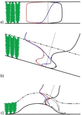
was originally postulated-and closely related situations. First, consider the case of a

pressure driven fl_{ow through a parallel two-dimensional duct fully occupied by}

vegetation (Figure 1a). This case, modelled in a wind tunnel by Seginer at al. (1976), is

sufficiently closely related to real-world canopy fl_{ows that any successful canopy}

closure should provide at least qualitatively accurate results. Similar to Poiseuille fl_ow,

symmetry demands that the shear stress goes through zero at the duct centreline, where

u

1 reaches a maximum, and has opposite signs on the two sides of the centreline so

that momentum fl_{ows towards the walls from the velocity maximum. In contrast the}

velocity-squared closure results in a maximum in shear stress on the centreline , where it

should be zero, and is zero on the walls where it should be maximal. Furthermore, the

ambiguity in the sign of the closure means that the momentum fl_{ux is in one direction}

only rather than changing sign on the centreline. This ensures that, for this example, the

parameterized fl_{ow also fails condition IV since the product of the rate of working of the}

shear stress, which, like u

1 has a single sign, and the rate of strain∂ u1 ∂x3, which is

asymmetric across the duct, is zero.

Next consider fl_{ow over hills covered with canopies subject to diabatic and}

hydrodynamic pressure gradients. Two fl_{ow patterns are commonly observed in these}

situations, gravity currents with wind speed maxima within the canopy driven by

hydrostatic pressure gradients (e.g. Goulden et al., 2006, Oldroyd et al., 2014) and

reversed fl_{ow in the lee of the hill caused by the hydrodynamic pressure gradient in} fl_{ows near neutral strati}fi_{cation (e.g. Poggi and Katul 2007a,b). Gravity currents}

generated when radiative cooling produces a layer of higher-than-ambient density on a

slope are ubiquitous at night. (Belcher et al., 2008, 2012). The gravity current/wall jet

then is a case of great practical importance for flux tower studies but one where the

phenomenon is unequivocally pressure driven (in contrast to turbulent transport driven).

As in the duct case above, the velocity-squared closure produces a maximum in shear

stress at the velocity peak, where physically the shear stress should be close to zero

the maximum in the gravity current windspeed, the shear stress is positive (upward

momentum transfer), acting to remove momentum from the gravity current and balance

the pressure gradient (e.g. van Gorsel et al. 2011). As shown in Figure 1b, the

velocity-squared closure sees momentum being transferred towards the velocity peak,

accelerating the current.

Our third example, fl_{ow separation, occurs when the combined effects of canopy drag}

(or surface friction) and an adverse pressure gradient reduce streamwise momentum

faster than turbulent transfer of momentum from faster moving air aloft can redress the

balance. Eventually a point is reached where the fl_{ow stops and reverses, creating a}

separation bubble. Modelling this requires capturing the balance between

cross-streamline momentum transport and the pressure gradient. Since the velocity-squared

closure predicts zero shear stress at the edges of the separation region, where it should

be large or even maximal (Poggi and Katul 2007a,b), incorrect predictions of this

balance occur. As a result, the size of the recirculation bubble cannot be accurately

predicted (see Figure 1c).

These three important practical examples show that not only is the velocity-squared

closure fl_{awed at a basic level, in that it fails conditions I, II III and IV, but it also fails}

to meet condition V and regularly produces unphysical predictions. Consequently, we

conclude that its use in modelling complex canopy flows is fundamentally wrong.

5. Summary and Conclusions

Although the defi_{ciencies of} fi_{rst order closures for modelling complex turbulent} fl_ows

and simple canopy fl_{ows are well known, they remain attractive when the main}

requirement is simplicity and if their shortcomings are well understood. Five

requirements that such closures must satisfy, if they are to be used reliably in complex

fl_{ow models, have been defined: they must be tensorially invariant, unambiguous,}

complete, globally satisfy the second law of thermodynamics and not lead to unphysical

results. The most popular and well-tested fi_{rst order turbulence closures are based on}

the eddy diffusivity concept. Such models treat the averaged turbulent flow as a linear

24 

the turbulent flow is Stokesian. In reality, as discussed in section (3), canopy flows

depart from this idealization in two ways: non-local dependence of stress on rate of

strain and the viscoelastic response of the turbulent stresses to straining.

The Finnigan and Belcher (2004) group of models for canopy fl_{ow in complex terrain}

uses the mixing length approach to define an eddy diffusivity. This carries a set of

implicit assumptions not all of which are automatically satisfi_{ed in all plant canopies,}

and so places conditions upon the closureÕs use. The methodology for deriving the

diffusivity using mixing-lengths was introduced almost 90 years ago and has been

developed and tested extensively since then. Despite the problems that are peculiar to

canopies, mixing lengths can be defended if their formulation is linked to the dominant

eddies responsible for turbulent transport in a robust way. Tensorially-invariant eddy

diffusivity models based on mixing lengths satisfy four of the five conditions we have

stipulated, and where they fail the fifth condition by giving unphysical results, it is

because of defi_{ciencies that are well understood so that their failure can be anticipated.}

The velocity-squared first order closure scheme proposed by Yi et al. (2005) and Yi

(2008) has a different form to the eddy diffusivity approach. This closure fails to satisfy

any of the five conditions in both simple and complex canopy flows. In particular it is

ambiguous (without further stipulations) and neither tensorially invariant nor material

frame indifferent, rendering it immediately problematical for use in complex flows

where simplified equations are typically derived using coordinate transformation. More

fundamentally, the three hypotheses on which the closure is founded and which are

proposed as principles of fluid mechanics (see Yi, 2008) can each be shown to be

incorrect by straightforward examples.

All Reynolds stress closures are engineering approximations and those most appropriate

to a particular problem need to be tailored to the circumstances. The success of

two-equation models that employ sophisticated eddy diffusivities or of higher order closure

models in engineering applications depends in part on the availability of more tunable

constants as the degree of the closure increases (eg. Hanjali«c and Kenjereš_{, 2008). In}

suitable for analytic modelling of complex canopy flows. In reality the desire for an

analytic solution (or at least a transparent numerical solution) limits us to situations

where the complexity can be treated as a small perturbation to a simple background

shear flow. Nevertheless, the small perturbation equations must be derived by a rational

simplification process from the general case and this inevitably requires coordinate

transformations and turbulence closures that, at a minimum, do not violate the five

principles we have set out. We have paid particular attention to mixing length-based

closures but this does not imply that there are no other appropriate closure schemes for

canopy fl_{ows in complex terrain. For example the approaches of Cowan (1968) or}

Massman (1997) could be generalized to be complete and invariant. In contrast, the

fundamental and practical issues associated with the velocity-squared closure means that

its use or any conclusion derived from it is unsound.

Appendix Derivation of a tensorially invariant first order closure

Following Aris (1962), we have referred to a fluid whose stress tensor is linearly

dependent on its rate of strain tensor as Stokesian. Such a relationship requires the fluid

to have certain properties. In the steps below we derive these properties in the course of

moving from a completely general constitutive relationship to a scalar eddy diffusivity

so as to clarify the assumptions we are making about the behaviour of the averaged

turbulent field. The necessary steps are essentially those used to derive the form of the

viscous stress in a Newtonian fl_{uid (Batchelor, 1967) or that follow from the}

requirements of rational mechanics (Lumley, 1978) or the equivalent steps used to

derive sub-fi_{lter scale closures in Large Eddy Simulations (Wyngaard, 2010). Note to}

begin with that the simplest conceptual fi_{rst order closure relates} σ

ij directly to ui but the need for Galilean invariance precludes this approach. Instead we wish to derive a

linear relationship betweenσ

ijand ∂ ui ∂xj while preserving tensor invariance.

We split the stress tensor into the sum of its isotropic and anisotropic parts

σ

ij=dij+

1

3

σ

kkδij     (20) 

26 

well as ÔdeviatoricÕ normal stresses that sum to zero (Batchelor, 1967). Both d_ijand

∂ _ui ∂_x

jare second order tensors so linear dependence takes the general form,

d_ij = A_ijkl∂ _uk ∂x_l      (21) 

where the fourth order tensor A_ijklis a property of the local state of the turbulent fl_{ow but}

does not depend directly on u

i or its spatial derivatives. Since dijis symmetric in the

indices i and j, so isA_ijkl.

Splitting the deformation tensor into the sum of its symmetric and antisymmetric parts

we obtain,

∂ u_i ∂x_{j =1 2⎣}⎡∂ u_i ∂x_j+∂ u_j ∂x_i⎤_{⎦+1 2}⎡_⎣∂ u_i ∂x_j− ∂ u_j ∂x_i⎤_⎦ =Sij−1 2εijkωk

(22)

where ε

ijkis the alternating tensor and ωk the mean vorticity. The anisotropic

component of the stress tensor is then,

d_ij=A_ijkle_kl −_{1 2A}

ijklεklmωm     (23) 

Equation (23) can be simplifi_{ed considerably if we assume that A}

ijkl, as well as being

symmetric in i and j, is isotropic in the sense that the deviatoric stress generated in an

element of fl_{uid by the deformation} ∂ _ui ∂_x

jis independent of the orientation of the

fl_{uid element. This is another way of saying that the fluid itself has no preferred}

direction and in general this is not true of volume-averaged turbulent canopy fl_{ow, for}

two reasons. First, if the orientation of the solid canopy elements is predominantly in

one direction then deformation along axes parallel or normal to the elements may

produce different stresses. Second, the quadratic nature of canopy pressure drag (2)

indicates that the simplest symmetry of turbulent canopy fl_{ow is not isotropy but}

axisymmetry with the axis aligned with the mean fl_{ow (Finnigan, 2000). However, if we}

assume that the turbulent flow is isotropic in the sense given above, the coefficient

products of the basic isotropic second order tensor, the Kronecker delta,

Aijkl =µδikδjl+µ′δilδjk+µ′′δijδkl     (24) 

where µ,µ_′,µ_′′ are scalar coefficients and, since we require A_ijkl to be symmetrical in i

and j, then µ =µ_′. Aijkl is now symmetric in k and l also and the term containing

ε_klmω_{m drops out of (23) because of the properties of the alternating tensor, leaving ,}

dij=2µeij+µ′′eiiδij     (25) 

Finally, since from continuitye

ii=0, a tensorially invariant closure can be written as,

σ

ij−σkkδij 3=K

(

∂ ui ∂xj+∂ uj ∂xi

)

=2KSij

(26)

The non-isotropic part of the turbulent stress tensor is thus linearly proportional to the

mean rate of strain tensor, with the scalar eddy diffusivity K. As Sijonly involves

velocity gradients and K is a scalar, the expression for σ

ijremains Galilean invariant.

This derivation illustrates that the familiar tensorially invariant form of the fi_{rst order}

stress closure required the assumption that the mean turbulent stresses in the Ôfl_uidÕ

defi_{ned by time and spatial averaging across the multiply connected canopy airspace had}

an isotropic response to straining and that S

ii=0. If, in contrast, we had assumed that

the response of a fl_{uid element to straining was axisymmetric rather than isotropic, the}

simplest expression for σ

ijwould involve two independent terms even when Sii =0 (Batchelor, 1953; p43; Finnigan, 2000).

References

Aris R. (1962) Vectors, Tensors and the Basic Equations of Fluid Mechanics. Dover

Publications Inc., New York. 286pp.

Bai, K., Meneveau, C. and Katz, J. (2012) Near-wake turbulent flow structure and

mixing length downstream of a fractal tree. Boundary-Layer Meteorol., 143: 285-308

Boussinesq, J., 1877: Theorie de lÕecoulement tourbillant. Mem. Presente«s Acad. Sci. Paris, 23, 56Ð58.

Batchelor, G.K (1953) The Theory of Homogeneous Turbulence. Cambridge University

Press, Cambridge. 197pp.