Solar Resource Estimation Using a Radiative Transfer with Shading (RTS) Model

This is a repository copy of

Solar Resource Estimation Using a Radiative Transfer with

Shading (RTS) Model

.

White Rose Research Online URL for this paper:

http://eprints.whiterose.ac.uk/91560/

Version: Accepted Version

Proceedings Paper:

Gooding, J, Smith, CJ, Crook, R et al. (1 more author) (2015) Solar Resource Estimation

Using a Radiative Transfer with Shading (RTS) Model. In: EU PVSEC 2015 Conference

Proceedings. European PV Solar Energy Conference and Exhibition 2015, 14-18 Sep

2015, Hamburg, Germany. , 2800 - 2805. ISBN 3-936338-39-6

https://doi.org/10.4229/EUPVSEC20152015-6AV.4.25

[email protected]

https://eprints.whiterose.ac.uk/

Reuse

Unless indicated otherwise, fulltext items are protected by copyright with all rights reserved. The copyright

exception in section 29 of the Copyright, Designs and Patents Act 1988 allows the making of a single copy

solely for the purpose of non-commercial research or private study within the limits of fair dealing. The

publisher or other rights-holder may allow further reproduction and re-use of this version - refer to the White

Rose Research Online record for this item. Where records identify the publisher as the copyright holder,

users can verify any specific terms of use on the publisher’s website.

Takedown

If you consider content in White Rose Research Online to be in breach of UK law, please notify us by

SOLAR RESOURCE ESTIMATION USING A RADIATIVE TRANSFER WITH SHADING (RTS) MODEL

James Gooding, Christopher J. Smith, Rolf Crook and Alison S. Tomlin

Energy Research Institute, School of Chemical and Process Engineering, University of Leeds Leeds LS2 9PR, United Kingdom

ABSTRACT: A combination of falling technology prices and government financial incentives has led to the rapid expansion of the solar microgeneration industry in the UK and around the world. With conditions for investment becoming more favourable, viability appraisal is now of great interest to potential investors ranging from individuals to large companies and authorities. A methodology to predict solar resource available to solar technologies in urban areas is presented that combines a radiative transfer simulation with shading derived from digital surface model (DSM) data. The radiative transfer simulation includes water vapour, ozone, clouds and surface albedo determined from MODIS satellite products along with aerosol properties that are derived from the GLOMAP model. A DSM is used to calculate the height of near-by obstacles and the horizon from each point of interest to establish when the site is in shade during a year. The site-level radiance field is adjusted by elements in shade and integrated over the view hemisphere of the photovoltaic (PV) panels to take into account panel tilt. Modelled annual global radiation (Wh/m2/a) estimations are validated using power output data from 17 sites across four major UK cities (Bristol, Cambridge, Leeds and Sheffield) and show good agreement with -3.68% and +2.62% mean percentage error under assumed performance ratio conversions of 0.75 and 0.8 respectively. The results are compared to the outputs of both Esri ArcGIS and PVGIS, the first of which predicted annual global radiation with -15.97% and -20.78% mean percentage error with the latter returning +3.34% and +10.23% mean percentage error for the 0.75 and 0.8 performance ratios.

Keywords: Solar Resource Estimation; Integrated Radiance Model; DSM; LiDAR; PV

1 INTRODUCTION

Microgeneration has already demonstrated substantial potential to become a significant contributor to the UK’s energy mix and could form an important part of meeting the UK’s 15% renewable energy by 2020 target set by the European Commission [1]. Of the microgeneration technologies available, solar photovoltaics (PV) have shown the most potential to meet energy demand. At the end of June 2015, UK installed capacity was 3.15 GW from a total of 712,594 installations [2].

As the microgeneration market has grown so too has interest in predicting the viability of PV at individual properties, leading to an increasing number of academic and industry studies of solar resource. One popular methodology is the European Solar Radiation Atlas (ESRA) model [3-5] that was used to create the popular European Union Joint Research Council (EU JRC) PVGIS solar databases and has been incorporated into the open-source GRASS Geographic Information System (GIS) software by Hofierka and Šúri [6] in the r.sun routine [7]. This model of annual global irradiance has three major components: the estimation of clear-sky global irradiation for a horizontal surface and a clear-sky index; the calculation of diffuse and direct components of overcast global irradiation; and the conversion of horizontal surface global irradiation estimations for inclined surfaces [8,9]. The model incorporates the interaction of solar radiation with geometrical, topographical and atmospheric constitutional factors. The Earth’s geometrical properties alter the calculation of solar irradiance as they determine the declination, latitude and solar hour angle of a site of interest. Terrain features include the elevation, inclination and orientation of a site as well as shading interactions from major surrounding topographical features. The atmosphere scatters and absorbs solar radiation in a variety of processes through interactions with gases, particulate matter and condensed water in clouds. The EU JRC PVGIS model incorporates these processes using the Linke turbidity factor (TLK) [10]

which is derived from satellite measurements of atmospheric matter such as cloud water vapour, ozone and aerosol particles.

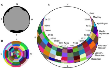
Figure 1 A: Example viewshed model in which parts of the sky that are obstructed from view are shown in black. B: A sky map. C: A sun map for 53.8° latitude.

The viewshed model shown in Figure 1A can be used to determine if the point of interest is exposed to direct radiation once the position of the Sun is established in the hemispherical coordinate system. Sun position can be calculated using a latitude-defined Sun map Figure 1C in which each coloured polygon, called a Sun map sector, represents the approximate position of the Sun for a half-hour period of the day in a specific month. Overlaying the viewshed model onto the Sun map shows the times of a year when the Sun is visible from the point of interest and is exposed to direct radiation. Equation (1) from Fu and Rich [15] is used to estimate direct radiation ( , )

for each of the sun map sectors that are not completely obscured by the viewshed model:

,

= ( )

, , cos ,

(1)

where is the solar constant (1367 W/m2),

, is the time duration represented by the

sunmap sector and , is the gap fraction for the

sun map sector. Gap fraction is the proportion of visible sky for each sector. , is the angle of incidence

between centroid of sky sector and axis normal to the surface and ( )_{is the transmittivity of the atmosphere}

with respect to the optical path, calculated using:

( ) = ( . . × ), (2)

in which is height above-sea-level in metres. The result is the direct radiation at the sun map sector’s centroid zenith angle ( ) and its azimuth angle ( ).

In contrast to direct radiation, diffuse radiation is received from all visible parts of the sky. Fu and Rich [13] overlay the viewshed model onto a uniformly divided hemispherical perspective of the sky (Figure 1B) to determine which parts of the sky contribute diffuse radiation to the point of interest. For each sky map sector that is not completely obscured by the viewshed model, diffuse radiation ( , ) is obtained from:

, =

, , cos ,

(3)

where Rglbis the global normal radiation given by:

=

( )

1 , (4)

in which is the proportion of global normal radiation flux that is diffused, is the half-hour time interval for analysis and , is the gap fraction for sky sector.

In equation (3), _, is the proportion of diffuse radiation originating from a given sky sector which is calculated in one of two ways depending on the selection of the user. The default uniform sky diffuse model has incoming diffuse radiation the same from all sky directions such that:

, =

(cos cos )

. (5)

In the standard overcast model, however, the incoming diffuse radiation flux varies with zenith angle so that:

,

= (2cos + cos 2 2cos cos 2 )

4

(6)

in which and are the bounding zenith angles of the sky sector and is the number of azimuthal divisions in the sky map.

Diffuse irradiance is calculated by summing the estimations of _, for all sky map sectors that are not completely obscured by the viewshed model. Finally global irradiation is the sum of both the direct and diffuse estimations.

Gueymard [18] provides a detailed comparison of clear-sky irradiance predictions from 18 solar radiation estimation methodologies including Fu and Rich [13] and Hofierka andŠúri [6]. Gueymard ranks Hofierka andŠúri [6] as the 8th most accurate clear-sky irradiance estimation method with Fu and Rich [13] in last place, concluding that solar radiation routines included in existing GIS software are based on models that are of low or limited performance [18]. It is important to note that whilst the validation sites used in Gueymard [18] are renowned for the quality of insolation data captured, they are inconsistent with the urban locations at which solar microgeneration technologies are most commonly installed. For example, they are not subject to the same degree of shading from surrounding objects and topographical features as typical urban and suburban roofs and so it is important to investigate the accuracy of the proposed solar insolation estimation method against other methodologies in the context of urban areas. Of the solar resource estimation methodologies to utilise either the EU JRC PVGIS database or ArcGIS mentioned above, only Šúri et al. [4] attempts to validate the findings of the solar insolation predictions. However, their validation utilises a meteorological model accurate to a resolution of 1 km2and is not compared to physical measurements inside the study area.

software, and Hofierka andŠúri [6] that has been used in the EU JRC PVGIS webtool and solar radiation databases. The Fu and Rich methodologies will be referred to hereafter as FuRich whilst the methodology behind the EU JRC PVGIS webtool will be referred to as PVGIS. The method presented in this work will be referred to as RTS (Radiative Transfer with Shading).

This article describes a methodology combining an integrated radiance model with a DSM-derived shading model to create a solar resource appraisal method suitable for urban areas. The use of a DSM to define shading is a significant development from PVGIS which does not include shading from objects surrounding a site explicitly by default. Furthermore, PVGIS uses cloud reflection derived from satellite data to adjust clear-sky irradiance estimation. By contrast, RTS takes satellite derived cloud properties such as optical depth and cloud fraction and incorporates them directly into the radiative transfer equation. For these reasons, RTS is also far more detailed in its consideration of factors that affect annual global solar radiation than FuRich as will now be explained.

2 METHOD

2.1 Theoretical basis

A diffuse radiance field with a modification for shading was used to calculate the angled insolation at each site. The model uses the DISORT radiative transfer code [19] with a pseudo-spherical correction to improve accuracy at low Sun angles. The direct beam irradiance is attenuated by atmospheric ozone and water vapour which is provided on an 8-day average basis from the MODIS Terra and Aqua satellite data on a 1°×1° global grid. Morning conditions are provided by the Terra platform that overpasses the equator approximately 10:30 am local solar time each day, and Aqua provides the afternoon observations passing over the equator at around 1:30 pm local solar time. This allows diurnal effects to be replicated in the simulations. Aerosol extinction, single scattering albedo and phase function is introduced by the GLOMAP model [20] that includes optical properties in 6 shortwave spectral bands for 4 aerosol species in 4 particle size modes. Cloud fraction, effective droplet radius, and cloud water content for liquid and ice are also provided from MODIS Terra and Aqua. Finally, surface albedo for 7 shortwave spectral bands is supplied on a 0.05°×0.05° grid using combined Terra and Aqua data every 8 days as a 16-day moving average.

From the atmospheric and land inputs the radiative transfer simulation is run for the midpoint of each hour for each 8-day period of 2013 to produce the ground-level radiance field along with the direct horizontal irradiance , diffuse horizontal irradiance and ground-reflected irradiance .

Radiances are calculated on a discrete grid of 3° in the polar direction and 10° in the azimuthal direction giving a total of 61×36 angular bins where the polar angle runs from 0° to 180° to capture both downwelling and upwelling radiances. To calculate tilted irradiance the angular contribution of diffuse radiances emanating from each 3°×10° sky bin is summed and added to the direct irradiance contribution:

= , + cos

cos (7)

where

= max 0, cos cos sin

+ sin sin cos (8)

is a spherical geometry weighting ensuring that only radiances in the hemisphere of panel view are counted, and is the solid angle of summation (3°×10°) in steradians. is the panel tilt angle, is the panel azimuth angle, is solar zenith angle and is solar incidence angle. The sum approximates the integration of radiances as the limit approaches zero.

For roof spaces of less than 200 m2a single viewshed model is generated for the location of the PV panels. Variation in shading across large installations on roofs of more than 200 m2 is accounted for through the calculation of hemispherical viewshed models for every 25 m2that are then combined as follows. The heights of the horizon for each of the 32 search directions from each hemispherical viewshed model across the roof space are averaged to generate a mean hemispherical viewshed model, which is produced on a flat x-y grid of 201×201 pixels. This is then converted into a polar representation and binned into the same 3°×10° resolution as the radiance field. Each pixel in the 201×201 x-y grid is defined as unobstructed, obstructed, or outside of the hemisphere. For each bin the fraction of unobstructed pixels to the total pixels in that bin is used to calculate a skyview fraction for each of the 61×36 angular bins.

The radiance field is produced assuming a homogeneous flat surface and needs to be adjusted to take into account the obstructed horizon. The direct irradiance is a simple scaling of the skyview fraction for the bin the Sun resides in for the hour in question, becoming = . The diffuse sky irradiance is more complex as it emanates from all bins of the sky yet is not generally isotropic. Radiances from fully or partially obscured directions are reduced by that sky bin’s skyview fraction and then summed over a horizontal plane such that the diffuse horizontal irradiance becomes

= , , (9)

with = 0°in the definition of and the sum over i runs only to 30 (polar angle 90°) as no upwelling radiances are required for horizontal downwelling calculations. The adjusted total downwelling horizontal irradiance due to horizon shading is modelled as

= +

+ . (10)

The next stage is then to replace the radiances from fully or partially obstructed bins with a weighting between the ground-albedo radiance value / and the original diffuse sky radiance value and to multiply all the radiances by the hemispherical shading factor such that

, = , , +

1 ,

assuming that the surface albedo of the ground and the obstruction are the same. Finally the shading-adjusted tilted irradiance is derived by substituting the , from equation 11 back into equation 7 and replacing with in the same equation, to give

= , + cos

cos . (12)

2.2 Validation Data

The model has been validated using performance data from 17 PV installation sites across Bristol, Cambridge, Leeds and Sheffield in the UK. Figure 2 describes the distributions of azimuth (A) and slope (B) which were measured using DSM data of the validation sites and geo-referenced aerial photography. Array size (C) and power generation for 2013 (D) provided by the installation owners are also shown.

Figure 2 Frequency plots of orientation (A), slope (B), system size (C) and power output for 2013 (D) attributes of validation sites

The performance of the installations at each validation site has been provided in terms of annual power output for 2013 whilst the models return estimations of annual global insolation. Therefore, a performance ratio (PR) is applied to estimate the annual power delivered by solar modules as a function of their rated power and global insolation. The PR is a measure of the actual power output of a module compared to its performance at standard testing conditions, and takes into account all system losses such as from the inverter and the effects of elevated cell temperature. The literature contains a range of PR values with Pearsall and Gottschalg [21] suggesting 0.8 to 0.85, PVGIS using 0.75 [22] and Ayompe et al. [23] using experimental data to show that PR is approximately 0.8 for most of the year but slightly higher in November to January. Owing to the popularity of the EU JRC PVGIS tool, 0.75 has been selected as a lower bound PR value whilst 0.8 is also used as it better reflects the opinion of the scientific community.

2.3 Implementation of Existing Methodologies 2.3.1 FuRich

The solar radiation tool within the Esri ArcGIS software was run for the validation sites in each city using a DSM of 2 m horizontal resolution. The latitude input was set to match the location of the relevant validation site. The time configuration was set to “whole year with monthly interval” and the year was set to 2013 to match the

available validation data. All other options were left as default. The tool outputs an estimation of annual global solar radiation (Wh/m2/a) for each validation site.

2.3.2 EU JRC PVGIS

The EU JRC PVGIS webtool was used to estimate annual global solar insolation (Wh/m2/a). The locations of the relevant validation sites were found using the webtool map and a marker placed at the location of each installation. The appropriate slope, azimuth and system rating (kWp) were entered and the building mounted option selected. All other options were left as default. The webtool returned a webpage of annual global radiation predictions in kWh/m2 with a monthly breakdown.

3 RESULTS AND DISCUSSION

The percentage error in annual global radiation was calculated for each site using:

% = × 100 (13)

where n=17 is the number of sites, is modelled annual global irradiance and is the estimated irradiance at the site following the PR conversion. The subscriptTdenotes tilted irradiance as in equation (12).

3.1 Performance

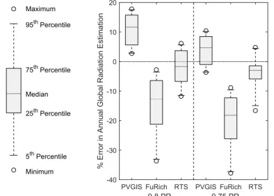
Figure 3 shows the performance of the RTS, PVGIS and FuRich methodologies under the assumed PRs of 0.8 and 0.75. The RTS model shows good agreement with the validation data with mean percentage errors of +2.62% and -3.68% under the 0.8 and 0.75 PRs respectively.

Figure 3 Percentage error of annual global radiation estimation for all three methodologies under both performance ratios.

The performance of PVGIS and FuRich are significantly poorer than RTS under the 0.8 PR. FuRich has a -15.97% mean error under the 0.8 PR whilst PVGIS has a +10.23% mean error. Although PVGIS performs better under the 0.75 PR, with +3.34% mean error, FuRich performs worse and incurs -20.78% mean error.

towards 0% error as for the RTS data. At three sites, FuRich generated an error in annual global radiation that was greater than +30% under the 0.75 PR. The largest error produced by RTS was 16.62% under the 0.75 PR at a site which also produced abnormally large errors for the PVGIS method under both PRs. The second largest RTS error was more typical of the worst overestimations at 11.8% which is considerably smaller than the errors encountered under FuRich. FuRich produced the largest inter-quartile ranges with the strongest bias toward underestimation of annual global radiation.

The results show that PVGIS under a 0.75 PR better approximates annual global insolation than when it is used with a PR of 0.8. This may be due to the lack of a shading model in PVGIS that leads to higher estimations of power output before the PR is applied. Despite the good performance of PVGIS under the 0.75 PR, a smaller mean percentage error is achievable when the RTS method is applied with a 0.8 PR and this value of PR is also better supported by the literature [24-26].

3.2 Insolation Estimation Sensitivity to Shading

The resolution of the baseline radiation calculations is approximately 5.6 km latitude by 3.2 km longitude, meaning that the majority of validation sites for each city lie within the same cell. Therefore, the RTS method of incorporating slope, azimuth and shading is highly important in solar insolation estimation. Due to the small number of validation sites and constrained combinations of azimuth and slope arrangements, it is not possible to comprehensively examine the role of the two geometrical parameters in the accuracy of solar insolation estimation under RTS. However, the effect of applying the DSM-derived shading model on the accuracy of annual global insolation prediction has been investigated using a mean absolute % error:

%

=1 × 100 (14)

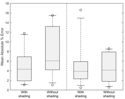
Figure 4 shows a reduction in the mean absolute percentage error for both PRs when the shading model is integrated with the radiance model.

Figure 4 Mean Absolute % Error in annual global radiation estimation with and without shading under both performance ratios

Under the 0.8 PR, a mean absolute error of +8.02% occurred when shading was not considered which is greater than the +2.62% absolute mean percentage error when the shading model was applied.

It is important to note here that RTS without shading still outperformed the mean absolute percentage error incurred for both FuRich and PVGIS when the 0.8 PR, which is better supported by the literature, was applied.

3.3 Suitability to City-Scale Applications

The large resolution of the baseline radiation output (5.6 km latitude by 3.2 km longitude) means that one of the most computationally intensive parts of the method need only be executed once to cover a considerable area. Whilst the generation of viewshed models for properties within a study area of this size is likely to have considerable processing demands, the estimation of solar resource on a city scale using the RTS model is entirely achievable. This means RTS could be used to achieve greater accuracy in city-scale PV viability analysis than existing methodologies such as Gooding et al. [11].

4 CONCLUSION

A radiative transfer with shading (RTS) model has been presented that estimates annual global solar radiation with +2.62% and -3.68% mean percentage error under assumed performance ratios of 0.8 and 0.75 respectively when validated using annual power output data for the year 2013 from 17 sites across four cities in the RTS model outperformed both the Fu and Rich [13] methodologies incorporated into the Esri ArcMap solar radiation toolset, and the Hofierka and Šúri [6] methodology that underlies the European Union Joint Research Council PVGIS webtool and is the backbone of the open-source GRASS GIS r.sun function. FuRich incurred -15.97 and -20.78% mean percentage errors under the 0.8 and 0.75 PRs whilst the results for PVGIS were +10.23% and +3.34% mean percentage error for each PR.

Unlike PVGIS, the method could be applied on a city scale after a small degree of adaptation and therefore could be used to inform large numbers of investment decisions with greater accuracy than previously possible using the FuRich methodology.

5 REFERENCES

[1] DECC (2013) ‘Increasing the use of Low-carbon Technologies’, Department for Energy and Climate Change,

https://www.gov.uk/government/policies/increasing-the-use-of-low-carbon-technologies [Accessed 26/07/2013] [2] DECC (2015) ‘Monthly Feed-in Tariff Commissioned Installations by Month’, Department for Energy and

Climate Change,

[4] Šúri, M., Huld, T. A., Dunlop, E. D., Ossenbrink, H.A. (2007) ‘Potential of solar electricity generation in the European Union member states and candidate countries’,Solar Energy, 81 (10), 1295-1305

[5] Nguyen, H.T. and Pearce, J.M., (2010) ‘Estimating potential photovoltaic yield with r.Sun and the open source geographical resources analysis support system’,

Solar Energy, 84, 831–843.

[6] Hofierka, J., Šúri, M., (2002) ‘The solar radiation model for open source GIS: implementation and applications’, Proceedings of Open Source GIS-GRASS Users Conference, Trento, Italy

[7] Hofierka, J.,Šúri, M., Huld, T. (2007) ‘r.sun – Solar irradiance and Irradiation Model’, GRASS, http://grass.osgeo.org/grass65/manuals/r.sun.html, [Accessed 10/02/2015]

[8] EU JRC (2012) ‘Solar Radiation (Europe) in PVGIS: Computation Scheme of Solar Radiation Database’, http://re.jrc.ec.europa.eu/pvgis/, European Union Joint Research Centre,[Accessed 09/02/2014]

[9] EU JRC (2012) ‘Solar Radiation and GIS’,European Union Joint Research Centre

http://re.jrc.ec.europa.eu/pvgis/solres/solmod3.htm [Accessed 12/09/2015]

[10] Remund J., Wald L., Lefevre M., Ranchin T., Page J., (2003) ‘Worldwide Linke turbidity information’,

Proceedings of ISES Solar World Congress, 16-19 June, Göteborg, Sweden, CD-ROM published by International Solar Energy Society. Available from:

https://hal.archives-ouvertes.fr/hal-00465791/file/ises2003_linke.pdf [Accessed 12/09/2015] [11] Gooding, J., Edwards, H., Giesekam, J., & Crook, R. (2013) ‘Solar City Indicator: A methodology to predict city level PV installed capacity by combining physical capacity and socio-economic factors’, Solar Energy, 95(0), 325-335.

[12] Brito, M.C., Gomes, N., Santos, T., Tenedorio, J.A. (2012) ‘Photovoltaic potential in a Lisbon suburb using LiDAR data’,Solar Energy, 86 (1), pp.283-288

Esri (2014) ‘How Solar Radiation is Calculated’, Esri, http://resources.arcgis.com/en/help/main/10.2/index.html #//009z000000tm000000 [Accessed 08/12/2014] [13] Fu, P., Rich, P., (1999) ‘Design and implementation of the Solar Analyst: an ArcView extension for modeling solar radiation at landscape scales’, Proceedings of the 19th Annual ESRI User Conference

[14] Fu, P. (2000) ‘A Geometric Solar Radiation Model with Applications in Landscape Ecology’, Ph.D. Thesis, Department of Geography, University of Kansas, Lawrence, Kansas, USA.

[15] Fu, P., and P. M. Rich (2000) ‘The Solar Analyst 1.0 Manual’, Helios Environmental Modeling Institute

(HEMI), USA.

[16] Fu, P., and P. M. Rich (2002) ‘A Geometric Solar Radiation Model with Applications in Agriculture and Forestry’, Computers and Electronics in Agriculture

37:25–35.

[17] Rich, P. M., and P. Fu (2000) ‘Topoclimatic Habitat Models’, Proceedings of the Fourth International Conference on Integrating GIS and Environmental Modeling.

[18] Gueymard, C. A. (2012) ‘Clear-sky irradiance predictions for solar resource mapping and large-scale applications: Improved validation methodology and detailed performance analysis of 18 broadband radiative models’,Solar Energy, 86, 2145-2169

[19] Stamnes, K., Tsay, S.C., Wiscombe, W., Laszlo, I., (2000) ‘DISORT, a general purpose Fortran program for discrete-ordinate-method radiative transfer in scattering and emitting layered media: Documentation of methodology’, Dept. of Physics and Engineering Physics, Stevens Institute of Technology, Hoboken, NJ, USA. [20] Scott, C.E., Rap, A., Spracklen, D.V., Forster, P.M., Carslaw, K.S., Mann, G.W., Pringle, K.J., Kivekäs, N., Kulmala, M., Lihavainen, H., Tunved, P., (2014) ‘The direct and indirect radiative effects of biogenic secondary organic aerosol’,Atmospheric Chemistry and Physics, 14 (1), 447-470.

[21] Pearsall, N. and Gottschalg, R. (2012) ‘Performance Monitoring’ In: Sayigh, A. ed. ‘Comprehensive Renewable Energy’, Amsterdam: Elsevier, pp: 777 [22] EU JRC (2012) ‘Interactive Maps and Animations’,

European Union Joint Research Centre, http://re.jrc.ec.europa.eu/pvgis/imaps/index.htm,

[Accessed 08/12/2014]

[23] Ayompe, L.M., Duffy, A., McCormack, S.J., Conlon, M. (2011) ‘Measured Performance of a 1.72 kW Rooftop Grid Connected Photovoltaic System in Ireland’,

Energy Conversion and Management, 52, 816 – 825 [24] Reich, N. H. (2012) ‘Performance ratio revisited: is PR > 90% realistic?’, Progress in Photovoltaics: Research and Applications, 20 (6), 717-726

[25] Leloux, J. Navarte, L., Trebosc, D. (2012) ‘Review of the performance of residential PV systems in France’,

Renewable and Sustainable Energy Reviews, 16 (2), 1369-1376