An Analysis Framework for Inter-User Interference in IEEE 802.15.6 Body Sensor Networks: A Stochastic Geometry Approach

White Rose Research Online URL for this paper:

http://eprints.whiterose.ac.uk/98816/

Version: Accepted Version

Article:

Sun, W, Ge, Y, Zhang, Z et al. (1 more author) (2015) An Analysis Framework for

Inter-User Interference in IEEE 802.15.6 Body Sensor Networks: A Stochastic Geometry

Approach. IEEE Transactions on Vehicular Technology. ISSN 0018-9545

https://doi.org/10.1109/TVT.2015.2502324

[email protected] https://eprints.whiterose.ac.uk/

Reuse

Unless indicated otherwise, fulltext items are protected by copyright with all rights reserved. The copyright exception in section 29 of the Copyright, Designs and Patents Act 1988 allows the making of a single copy solely for the purpose of non-commercial research or private study within the limits of fair dealing. The publisher or other rights-holder may allow further reproduction and re-use of this version - refer to the White Rose Research Online record for this item. Where records identify the publisher as the copyright holder, users can verify any specific terms of use on the publisher’s website.

Takedown

If you consider content in White Rose Research Online to be in breach of UK law, please notify us by

An Analysis Framework for Inter-User Interference

in IEEE 802.15.6 Body Sensor Networks: A

Stochastic Geometry Approach

Wen Sun, Yu Ge, Zhiqiang Zhang*, and Wai-Choong Wong

Abstract—Inter-user interference occurs when multiple body sensor networks (BSNs) are transmitting simultaneously in close proximity to each other. Interference analysis in BSNs is challenging due to the hybrid medium access control (MAC) and the specific channel characteristics of BSNs. This paper presents a stochastic geometry analysis framework for inter-user interference in IEEE 802.15.6 BSNs. An extended Matern point process is proposed to model the complex spatial distribution of the interfering BSNs caused by the hybrid MAC defined in IEEE 802.15.6. We employ stochastic geometry approach to evaluate the performance of BSNs, considering the specific channel char-acteristics of BSNs in the vicinity of human body. Performance metrics are derived in terms of outage probability and spatial throughput in the presence of inter-user interference. We conduct performance evaluation through extensive simulations and show that the simulation results fit well with the analytic results. Insights are provided on the determination of the interference detection range, the BSN density, and the design of MAC for BSNs.

Index Terms—inter-user interference, body sensor networks, stochastic geometry, medium access control.

I. INTRODUCTION

Advances in wireless communication technologies and re-cent development in the miniaturized computing devices have empowered the implementation of body sensor networks (B-SNs). A BSN comprises multiple sensor nodes and a coor-dinator worn on a human body. Sensor nodes continuously monitor the physiological information of the human body and deliver it through the coordinator to the backbone network for further processing [1]–[3]. The IEEE 802.15.6 Working Group was formed to develop a dedicated wireless standard for BSNs [4].

Inter-user interference is incurred by simultaneous transmis-sions in multiple BSNs in the vicinity, which tremendously de-teriorates reliable communication in BSNs. Natarajan et al. [5] highlighted the existence of the inter-user interference, and found that such interference reduces packet delivery rate by

Copyright(c) 2015 IEEE. Personal use of this material is permitted. How-ever, permission to use this material for any other purposes must be obtained from the IEEE by sending a request to [email protected].

W. Sun is with the Department of Computer Science, National University of Singapore, Singapore 117576 (e-mail: [email protected].).

Y. Ge is with Institute for Infocomm Research, Singapore 138632 (e-mail: [email protected]).

*Z. Zhang is with Department of Computing, Imperial College, London, SW72aZ, UK (e-mail: [email protected]).

W.C. Wong is with the Department of Electrical and Computer Engineer-ing, National University of Singapore, Singapore 117576 (e-mail: [email protected]).

35% in the presence of eight or more interfering BSNs. In our previous work [6], we found that only 68.5% of data transmission meets the reliability requirement even in the off-peak period in a realistic BSN deployment case in hospital. Interference analysis in BSNs is beneficial for interference mitigation and network management. The interference at the intended receiver is determined by a number of stochastic pro-cesses including the random spatial distribution of interferers. Typically, multiple topologies of interferers are assumed for the interference analysis, e.g., hexagonal lattice and regular lattice [7], [8]. However, for BSNs, it is impossible to assume typical topologies as BSN users usually move around without mobility constraints.

of human body, signals transmitting over a BSN typically experience more severe attenuation as compared with that without the presence of a human body [14]. Michalopoulou et al. [15] investigated the effects of human body on signal transmission and derived performance metrics in the closed-form expressions. Kim et al. [16] analyzed and compared the effects of passerby movement types, in both outdoor and indoor environments, to capture the effects of user motions such as walking and running. Rician distribution is found as a good fit for channel model in the on-body transmission in a BSN.

However, the existing stochastic geometry analysis works cannot be applied to BSNs directly due to the following reasons: (1) BSNs typically employ the hybrid IEEE 802.15.6 MAC, which would lead to more complex geometrical dis-tribution of the interferers (when compared to a traditional wireless network with a single-structure MAC protocol) due to the coexistence of contention-based and contention-free nodes. (2) Due to the presence of human body, the desired link in a BSN user follows a different channel model from that of the interference link, i.e., transmissions between interfering BSNs. To the best of our knowledge, there is no existing works on the interference analysis considering the effects of hybrid MAC and the specific channel characteristic of BSNs.

In this paper, we present a stochastic geometry analysis framework of inter-user interference in IEEE 802.15.6 BSNs. The main contributions of this paper are as follows.

• Firstly, we propose a stochastic geometry model to

ana-lyze the effects of IEEE 802.15.6 MAC on the spatial distribution of the interfering BSNs. Compared to the existing stochastic geometry analysis [9], [17]–[19], we relax the assumptions that each node in the network follows the same MAC operation mode at a given time. In our study, although all the BSNs employ the hybrid MAC structure defined in IEEE 802.15.6, a specific BSN may operate at either contention-based or contention-free state at a given time in the absence of global synchronization. We analyze the effects of IEEE 802.15.6 MAC using an extended Matern point process.

• Secondly, we analyze the inter-user interference consid-ering the specific channel characteristics of BSNs. We derive outage probability and spatial throughput of BSNs, under the assumption that Rician fading channel model is adopted for on-body communication (intended signal transmission) and Rayleigh fading is explored for inter-body communication, i.e., interference.

• Thirdly, we conduct extensive performance evaluation

through simulations and validate the theoretical analysis. Based on the analysis, the interference detection range is optimized to achieve the maximum spatial throughput while the reliable transmission requirement is met. More-over, our study provides insights on the design of MAC for BSNs depending on the specific BSN applications. The remainder of this paper is organized as follows. Sec-tion II describes the network model. SecSec-tion III characterizes the inter-user interference in BSNs using stochastic geometry. In Section IV, we validate the theoretical works using

simu-lations, and provide implications on the detection range, BSN density and MAC design. Finally, Section V concludes the paper.

II. NETWORKMODEL

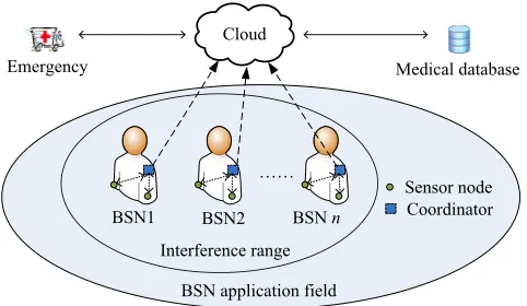
Fig. 1 illustrates the common architecture of BSNs. In a BSN, there is a single coordinator and multiple sensor nodes. BSN transmission is a two-tier communication, i.e., consisting of intra-BSN communication and inter-BSN com-munication. Intra-BSN communication is between the sensor nodes (including the coordinator) within a BSN, while inter-BSN communication is between the inter-BSN and the remote server. In particular, the physiological information collected by sensor nodes is first delivered to a coordinator within a BSN, which is referred to as intra-BSN communication. After that, the coordinator then forwards the information to the local or remote server for further processing, which is referred to as inter-BSN communication.

When BSNs move into the interference range of each other and transmit simultaneously, inter-user interference occurs. In other words, inter-user interference is the interference experienced by the intra-BSN communication of the current BSN from the intra-BSN communication of other BSNs in the same vicinity. As intra-BSN communication is between sensor nodes and the coordinator in a BSN, the source of the inter-user interference on the current BSN may be the transmission of either the coordinator or a sensor node of another BSN in the vicinity. As the intra-BSN communica-tion is typically coordinated by IEEE 802.15.6 MAC (see Subsection II-A), only a node transmits at a time. Thus an BSN communication will not be interfered by the intra-BSN communication within the same intra-BSN according to IEEE 802.15.6 MAC. For notational simplicity, in the rest of this paper, when we say a BSN transmits, it means that there is an on-going intra-BSN communication within the current BSN. The inter-BSN communication leverages on WLAN or cellular networks, which is different from that of the intra-BSN communication.

BSN2

BSN1 BSNn

Sensor node Coordinator Cloud

Medical database Emergency

BSN application field Interference range

……

A. IEEE 802.15.6 MAC Protocol

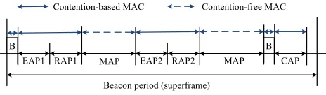
The IEEE 802.15.6 standard is specified to coordinate the intra-BSN communication [20]. We consider the beacon mode with superframes in this study. Fig. 2 shows the superframe structure. In IEEE 802.15.6, the entire channel is divided into superframe structures, which contains an active period and an inactive period. Each superframe is bounded by a beacon period of equal length. The active period is further divided into exclusive access phase 1 (EAP1), random access phase 1 (RAP1), managed access phase (MAP), exclusive access phase 2 (EAP2), random access phase 2 (RAP2), another managed access phase (MAP), and contention access phase (CAP)-in the order stated and shown above. At the beginning of the active period, the coordinator of a BSN synchronizes its sensor nodes by broadcasting a beacon packet. The beacon packet contains schedule information of the BSN. According to the beacon information, a sensor node that wishes to communicate during the EAP, RAP and CAP competes with other nodes using either a CSMA/CA or a slotted Aloha mechanism. The EAP1 and EAP2 are used for highest priority traffic such as reporting emergency events. The RAP1, RAP2, and CAP are used for regular traffic only. The Type I/II phases are used for uplink allocation intervals, downlink allocation intervals, bi-link allocation intervals, and delay bi-bi-link allocation intervals. In Type I/II phases, polling is used for resource allocation. In the MAP, nodes transmit in a contention-free mode in their allocated slots without competition. Sensor nodes are in sleep mode in the inactive period to save energy. The length of each time fraction, such as the RAP, MAP, CAP, EAP, etc. is determined by the parameters of the IEEE 802.15.6 MAC. The parameters could be adjusted according to the specific applications. The coordinator selects the boundaries of the superframe and thereby selects the allocation slots. The beacons are transmitted in every superframe. A sensor node could send information using either contention-based or contention-free scheme depending on the traffic type. As a BSN may have low channel utilization, duty cycle is defined to denote the percentage of the active period in a superframe. Typically, the hybrid MAC defined in the IEEE 802.15.6 standard comprises two categories of MAC protocols:

• Contention-free access mechanism: e.g. unscheduled

ac-cess, or scheduled access and variants, where a BSN transmits whenever there is a packet to be transmitted. In a MAP, nodes transmit using contention-free scheme.

• Contention-based access mechanism: e.g. CSMA/CA,

B B

EAP1 RAP1 MAP EAP2 RAP2 MAP CAP Beacon period (superframe)

Contention-based MAC Contention-free MAC

Fig. 2. IEEE 802.15.6 superframe structure, consisting of beacon transmission (B), exclusive access phase (EAP), random access phase (RAP) and contention access phase (CAP) periods. The EAP1 and EAP2 are used for highest priority traffic such as reporting emergency events. The RAP1, RAP2, and CAP are used for regular traffic only.

where a BSN transmits only if other BSNs within the detection range are detected silent.

Note that a node may have information that needs to be transmitted using contention-based and contention-free traffic at the according time slots. Although the analysis is performed for BSNs using IEEE 802.15.6 in this paper, it can also be applied to other networks where hybrid MAC mechanisms are employed, such as IEEE 802.15.4.

B. Channel Model

In a wireless channel, the signal experiences path-loss and fading before arriving at the intended receiver. The received signal strengthΩ (d)is given by

Ω (d) =G_·Ω0·h·d−α, (1)

whereG is a constant accounting for system loss, Ω0 is the

transmission power, h represents the fast fading factor, d is the distance between the transmitter and receiver, andαis the path-loss exponent.

Due to the blockage and absorbtion of human bodies, wireless signals are usually attenuated according to different channel models for on-body and inter-body communications. In particular, the path-loss exponent over on-body channels

αo is higher than that over the inter-body channels αI, i.e.,

2 < αI < αo [14]. Rayleigh fading has been widely used

in indoor environments, and thus is employed for inter-body channel model in this paper. For on-body channel, the fast fading of on-body channel model fits well with a Rician distribution [16].

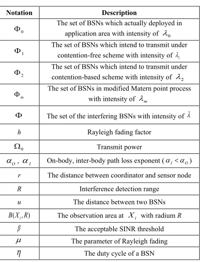
The notations and symbols involved in this paper are summarized in Table I.

III. INTERFERENCECHARACTERIZATION

In this section, we first describe the spatial distribution of the interfering BSNs, and then propose an extended Matern point process to model it. After that, we derive the outage probability and spatial throughput of BSNs in the presence of inter-user interference.

A. Spatial distribution of the interfering BSNs

We assume that BSNs are distributed uniformly and in-dependently in the BSN deployment area according to a homogeneous Poisson point process (with the intensity ofλ0). Denote the set of BSN locations asΦ0={X1, X2, ..., Xk, ...}.

The BSNs which intend to transmit at a given time can be divided into two categories:

• Φ1: the BSNs which intend to transmit under

contention-free scheme.Φ1also follows a Poisson point process with

the intensity of

λ1=w1ηλ0, (2)

• Φ2: the BSNs which intend to transmit under

contention-based scheme. Similarly, Φ2 follows a Poisson point

process with the intensity of

λ2=w2ηλ0, (3)

wherew2= 1₋w1. We have

Φ0= Φ1∪Φ2. (4)

Definition 1 (Interfering BSNs). The interfering BSNsΦ are defined as the BSNs which are transmitting effectively and simultaneously at a given time in the same channel, and hence, they may incur interference to one another.

For the contention-free scheme, the set of interfering B-SNs is exactly Φ1. For the contention-based scheme, a BSN

transmits only when other BSNs, either contention-based or contention-free based, are detected silent within the carrier sense range. Denote Φmas the set of interfering BSNs under

contention-based scheme. We have

Φ = Φ1∪Φm. (5)

Φ1∩Φm=∅. (6)

Fig. 3 shows an example of transmission status of B-SNs in the BSN deployment area. In this scenario, BSN2 and BSN4 may hold-on or back-off their transmissions due to the detection of the transmissions of BSN1 and BSN3 respectively, while BSNs under contention-free mode, e.g., BSN3 and BSN5, are able to transmit directly although they are close to each other. Thus without notating the location

TABLE I

THE NOTATIONS OF THE SELECTED TERMS.

TABLE I. THE NOTATIONS OF THE SELECTED TERMS

Notation Description

0

F The set of BSNs which actually deployed in

application area with intensity of l0 1

F The set of BSNs which intend to transmit under

contention-free scheme with intensity of l1 2

F The set of BSNs which intend to transmit under

contention-based scheme with intensity of l2 m

F The set of BSNs in modified Matern point process

with intensity of lm

F The set of the interfering BSNs with intensity of l

h Rayleigh fading factor

0

W Transmit power

O

a , a_I On-body, inter-body path loss exponent (aI<aO) r The distance between coordinator and sensor node

R Interference detection range

u The distance between two BSNs

( i, )

B X R The observation area at Xi with radium R

b The acceptable SINR threshold

m The parameter of Rayleigh fading

h

of the BSNs, we have the contention-free interfering BSN setΦ1 ={BSN3,BSN5,BSN6}, contention-base interfering

BSN set Φm = {BSN1}, and the total interfering BSN

set Φ = _{BSN1,BSN3,BSN5,BSN6_}. To model Φm in a

general case, we propose an extended Matern point process, described in the next subsection.

B. Extended Matern point process

As aforementioned, Matern point process models the spatial distribution of nodes using CSMA/CA. It is a non-independent thinning of the Poisson point process such that the distance between any two nodes in the Matern thinning is larger than a carrier sense range ofR. The node set selected in the Matern point process represents the nodes which effectively transmit using CSMA/CA at a given time, while the original Poisson point process represents the potential node distribution. This is accomplished by a hardcore process in Matern point process. In particular, each point of the original set is attributed an independent mark which is uniformly distributed in the interval [0,1]. A point xof the original set is selected in the Matern thinning if its mark is smaller than that of any other point of the original set within a range ofRaroundx. The hardcore process of Matern point process simulates the back-off mechanism in CSMA/CA, where only the nodes with the shortest back-off time withinRare allowed to transmit. The classic Matern point process cannot be applied directly in the interference analysis in BSNs as contention-free nodes are included in this case.

In this paper, we propose anextended Matern point process to represent the spatial distribution of the interfering BSNs under contention-based scheme in the presence of inter-user interference. LetΦm={X1, X2, ..., XM}be the set of BSNs

which are chosen for the extended Matern point process.Φm

is also an non-independent thinning of the original Poisson point process Φ2. It differs from the classic Matern process

as the selection of points inΦm does not only depend on the

contention-based setΦ2but also depend on the contention-free

BSN2 BSN 1

BSN3

BSN4

BSN5

R

BSN application field

BSN 6 BSNi

BSNj

shows a contention-based interfering BSN.

shows a contention-free interfering BSN.

shows a BSN which tries to transmit using contention-based scheme but backoff due to busy medium.

setΦ1. This captures the fact that BSNXi using

contention-based scheme is allowed to transmit when BSNs from both

Φ1 andΦ2 are detected silent within the open discB(Xi, R)

centered inXi and of radiusR. In particular, each point ofΦ2

is attributed to an independent mark uniformly distributed in the interval [0,1]. A tagged BSN Xi of Φ2 is selected inΦm

when the hardcore assigned to the tagged BSN t is smaller than that of any other point of Φ2 in B(Xi, R) and there is

no point ofΦ1 withinB(Xi, R).

The following terms are utilized to describe our model:

• Intensity is the spatial average of the number of BSNs

within a unit area. It is the same as the BSN density.

• Outage probabilityis the probability that SINR of a BSN is less than a threshold. It measures the performance of an individual BSN.

• Spatial throughput measures the number of BSNs that

transmit simultaneously and successfully within a unit area. It measures the overall performance of BSNs. C. The intensity of the interfering BSNs

Proposition 1 The intensity of the interfering BSNs using contention-based scheme, i.e., the BSN set thinning by the extended Matern point process, is given by

λm=

e−λ1πR2· (

1−e−λ2πR2 )

πR2 , R >0 (7)

whereλ1andλ2 are obtained from Eqs. (2) and (3),Ris the interference detection range.

Proof:In order to calculateλm, we first derive thespatial

probability of the interfering BSNs under contention-based mode.Spatial probabilityis defined as the ratio of the number of the transmitting BSNs to the number of BSNs which intends to transmit in a defined geographic area. Assume the Matern hardcore assigned to a tagged BSN i in the contention-based set Φ2 is m(Yi) = t. From the modeling of the extended

Matern point process, we know that BSN i is allowed to transmit when the Matern hardcore of other BSN j (j _̸= i) withinB(Yi, R)fromΦ2is larger thant, i.e.,m(Yj)> t, and

there is no BSN fromΦ1inB(Yi, R), i.e.,φ1(B(Yi, R)) = 0.

The integration is taken over all possible m(Yi) = t (from

0 to 1) and all possible number of BSNs in B(Yi, R), i.e., φ2(B(Yi, R)) =n. We get the spatial probability that BSN i

transmits by

ps=

∫ 1

0

∑

n∈N

Pr_{m(Yi) =t} ·Pr{φ1(B(Yi, R)) = 0}

·Pr    n ∏

j=1,j̸=i

m(Yj)> t|φ2(B(Yi, R)) =n, m(y) =t







·Pr_{φ2(B(Yi, R)) =n}dt (8)

=

1

∫

0

∑

n∈N

(λ2πR2₎n n! ·e

−λ2πR2_·e−λ1πR2_·(1−t)n_{dt (9)}

=e

−λ1πR2· (

1−e−λ2πR2 )

λ2πR2 , (10)

where φ1(B(Yi, R)) and φ2(B(Yi, R)) are the number of

BSNs under contention-free and contention-based scheme within B(Yi, R) respectively. Eq. (9) is by the fact that the

number of contention-based or contention-free BSNs near the tagged BSN follows Poisson distribution with intensity ofλ1

andλ2 respectively, i.e.,

Pr{φ2(B(Yi, R)) =n}=

(λ2πR2₎n n! ·e

−λ2πR2_,

Pr_{φ1(B(Yi, R)) = 0}=e−λ1πR

2

.

We arrive at Eq. (10) from Eq. (9) by employing the MacLau-rin series of exponential function. Thus we get the intensity of Φm (as shown in Proposition 1) by multiplying the spatial

probability ps with the intensity of BSNs under

contention-based scheme.

From Proposition 1, the extended Matern point processΦm

depends on the contention-free setΦ1, whileΦ1is independent

from Φm. The intensity of the interfering BSNs (Φ = Φ1∪

Φm) is the addition of BSNs under both contention-based and

contention-free schemes.

Lemma 1 The intensity of the interfering BSNs is given by

λ=λ1+λm. (11)

D. Outage probability

In the presence of inter-user interference, outage occurs when the SINR of a BSN is below an acceptable threshold

β, i.e.,

SIN R= hsr

−αo ΩI + Ωn

< β, (12) wherehs is the fading factor for the desired signal, r is the

distance between the coordinator and sensor nodes in a BSN,

ΩI is the interference power normalized with transmission

powerΩ0, andΩnis the average noise power, also normalized

with Ω0. We assume the noise is white noise, i.e., being

constant over the whole frequency band.

Proposition 2 The outage probability of a BSN with Rician fading for the on-body communication in the presence of inter-user interference is given by

Po=e(−Bs

δ −K₎

∞ ∑ m=0 ∞ ∑ n=0

(₋1)mJ(m, n)

m ∑ k=1 γm k k! (

Bsδ)k

,

(13) where

B=λcdE[hδI

]

Γ (1−δ), s= r

αo_β

2 , δ=

d αI

,

J(m, n) = K

m

n!Γ (m+n+ 1)

(_Kβrαo

2

)n

,

γkm= m

∑

n=1

(−1)n

(_m

n

)

(δn)m,

(x)_m,x(x−1)...(x−m+ 1),

Proof: Outage occurs when SINR is below a threshold

β. Denote the CDF of SINR regardingβasFSIN R(β). From

Eq. (12), the outage probability of a BSN regarding the SINR thresholdβ is

Po= 1−FSIN R(β) = 1−

∫ ∫

x≥0,y≥0,x/y≤β

fs(x)fI(y)dxdy

= 1−

∫ ∞

0

Fs(βy)fI(y)dy, (14)

wherefs(x)is the PDF of the desired signalx,fI(y)is the

PDF of the interference signaly, andFs(x)is the cumulative

distribution function (CDF) of the desired signal. This is the ratio of the desired signal (xin Eq. (14)) to the interference (y in Eq. (14)) is less than β, i.e., x/y_≤β, when the noise is negligible, i.e.,

∫ ∫

x≥0,y≥0,x/y≤β

fs(x)fI(y)dxdy=

∫ ∞

0

∫ βy

0

fs(x)fI(y)dxdy.

Firstly, we calculate CDF for the desired signal Fs(x).

From Eq. (1), we have the desired signal

x(d) =G·Ω0·hs·d−αo, (15)

wherehsis the fading factor of the desired signal.

As the desired signal experiences Rician fading, hs at the

intended receiver follows non-central chi-squared distribution. According to [21], we have the CDF of hs as

Fhs(x) = 1−exp

(

−2K₂+x

) ∞

∑

m=0

(_2K

x

)m/2

Im

(√

2Kx),

(16) where

Im(x) =

∞

∑

k=0

1

k!Γ (k+m+ 1)

(x

2

)2k+m

is the modified Bessel function. From Eq. (15), we have

Fs(x) =Fhs(xr

αo_),

(17) Substitute Eq. (16) and Eq. (17) in Eq. (14). We have

Po=

∞ ∑ m=0 ∞ ∑ n=0

e−KJ(m, n)

∞

∫

0

ynexp

(

−r αo_βy

2

)

fI(y)dy.

(18) Let s=rαo₂β, we have

Po=e−K

∞ ∑ m=0 ∞ ∑ n=0

J(m, n)

∞

∫

0

yme−syfI(y)dy

=e−K

∞ ∑ m=0 ∞ ∑ n=0

J(m, n) (₋1)m_LI(m)(s), (19)

where LI(s) is the Laplace transform of the interference

with the PDF of fI(y) andLI(m)(s) is the m-th derivative

of LI(s). The last expression is obtained considering the

property of derivative of Laplace transform.

According to Ref. [22], we have

LI(s) = exp

{

−

∫ ∞

0

E[1₋e−shIr− α]

λ(r)dr

}

= exp(₋λcdE

[

hIδ

]

Γ (1₋δ)sδ)

= exp(

−Bsδ)

, (20)

wherecd is the volume of the d-dim unit ball.

Then_LI(m)(s)is expressed as LI(m)(s) = exp(−Bsδ)·

m ∑ k=1 γm k k! (

Bsδ)k

. (21) Substitute Eq. (21) in Eq. (19), we obtain Proposition 2.

Corollary 1 The outage probability of a BSN with Rician fading for body communication and Rayleigh fading for on-body communication in the presence of inter-user interference can be expressed as Eq. (13) with a simplified B as

B= λcdπδ

sin (πδ). (22)

Proof: Eq. (12) considers the general channel model for the inter-body communication, i.e., interference channel model. When interference link experiences Rayleigh fading, it can be simplified as

LI(s) = exp

(

−λcdsδ πδ

sin (πδ)

)

. (23) Thus we get Corollary 1.

E. Spatial throughput

A specific metric in stochastic geometry [10] is spatial throughput which characterizes the density of the nodes which successfully transmit at a given time (i.e. BSNs in the context of this paper) within a unit area. Spatial throughput considers the successful transmission probability of a BSN as well as the spatial reuse. For example, according to Ref. [10], in the case of Aloha MAC network with half-duplex transceivers, the spatial throughput is expressed asp(1₋p) (1₋Po)[10],

wherep is spatial probability, (1₋p) is the probability that the intended receiver is listening (not transmitting) when the transmitter transmits, and(1₋Po)is the successful

transmis-sion probability. In a BSN where the receiver is in listening state when the transmitter is transmitting, the term (1−p)

is negligible. Moreover, we utilize the intensity of interfering BSNs, e.g. λ1 and λm, instead of the spatial probability p

in order to consider the ratio of contention-based traffic and contention-free traffic in IEEE 802.15.6 BSNs.

Corollary 2 The spatial throughput is given by

S= (λ1+λm) (1−Po). (24)

is determined by a number of factors, including the inter-ference detection range R, the traffic allocation w1, and the BSN intensity. Spatial throughput can also be described as

S = λ(1₋Po) Ψ when considering transmission rate Ψ of

the nodes, as shown in [23]. In this paper, we normalize the transmission rate without considering it in Eq. (24), as defined in [10].

IV. SIMULATION ANDNUMERICALRESULTS

We investigate the performance of BSNs in the presence of inter-user interference in the network simulator QualNet 5.0.2 [24]. The simulation results are compared with the analytical results to validate the analysis. After the simulation validation, we present the numerical results, which provide implications on the selection of the interference detection range, the MAC protocol design, and the BSN intensity.

A. Simulation settings

In the simulation, a coordinator and a sensor node form a BSN. The distance between the coordinator and the sensor node is set as 1 meter. The simulation settings are configured according to the IEEE 802.15.6 standard [4], as shown in Table II. In this study, we consider an on-body channel model for the desired link (the transmission between sensor nodes in a BSN) with Rician fading and a path-loss model with the path-loss exponent of αo. The parameters regarding Rician

channel model are set according to [15]. On the other hand, we consider an inter-body channel model for the interfer-ence link (the transmission between BSNs) with Rayleigh fading and a path-loss model with the path-loss exponent of αI (αI < αO). We consider the signal attenuates with

Rayleigh fading with standard deviation of 6.2 dB for inter-body communication [14]. We choose a radio data rate of 250 kbps and a superframe length of 0.1 second. For healthcare applications, the data rate requirements of commonly used sensor nodes are 5 kbps for Electrocardiograph (ECG) and Electroencephalography (EEG), and 1 kbps for temperature sensor, respiratory sensor, and pulse sensor [1]. The wireless noise floor is set as -90 dBm [25]. Considering the combined usage of those sensors in a BSN, we set the duty cycle to be 20% in the simulation. For simplicity, the traffic load for all the BSNs are set the same in a specific scenario.

We consider the typical BSN deployment in the emergency waiting room in a hospital scenario in Singapore1_{, where}

the average area occupied by each patient is from 0.2 to 1 square meters. Considering the general case where only partial patients utilize BSNs, multiple channels available, and the generic characteristic of low channel utilization (duty cycle), we assume the BSN intensity range is from 1 BSN per unit area to 5 BSNs per unit area. According to the comprehensive survey [1], BSN intensity varies from 0.1 to 5 (BSNs per unit area) depending on the specific BSN application. Each BSN moves according to the random waypoint model [26]– [28]. As pointed out by Gong and Haenggi [19], the random

1_{The configuration settings of Changi General Hospital and Tan Tock Seng}

Hospital in Singapore

TABLE II

THE PARAMETER SETTINGS OF THE SIMULATION IN INTERFERENCE ANALYSIS.

Transmission power W0(dBm) -10

BSN intensity l(# of BSNs per unit area) 1~5

Duty cycle of a BSN h (%) 20

Noise level W (dBm) -90

Path-loss exponent of on-body channel model aO 3.6

Path-loss exponent of inter-body channel model aI 3

The distance between coordinator and sensor node r (m) 0.6̚1.4

SINR threshold b (dB) 5~15

walk model does not affect the uniform property of the point distribution. Initially, all BSNs are uniformly deployed and then they move independently. To remove the effect of differing initial conditions on performance, we run the simulation fifty times with different initial conditions and then calculate the average results. We compare the results in the mobility case with that in the Poisson point process case. As there is no existing works on interference analysis using stochastic geometry, we conduct the comparison between the analytical and the simulation results. As the spatial throughput is the function of intensity of the interfering BSNs and outage probability, we only compare the theoretical results with the simulation results regarding these two metrics.

B. Simulation Results

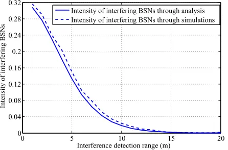
Fig. 4 shows the comparison of the intensity of the inter-fering BSNs obtained through simulation with that obtained through analysis by Eq. (7). As can be seen, both results are very close, except that the analytical results are a bit lower than the actual results, due to the reason that Matern point process cannot accurately estimate the CSMA/CA networks in certain situations. For example, if BSN1, BSN2, and BSN3 congregate together, BSN1 is silenced by its only neighbor BSN2, whereas BSN2 is in turn actually silenced by its neighbor BSN3. In the Matern model, BSN1 and BSN2 will not be retained, but if BSN1 and BSN3 are not neighbors and BSN3 has only BSN2 as neighbor, then CSMA/CA will allow BSN1 and BSN3 to transmit simultaneously. In [13], it is shown that only 78% of the transmitting nodes can be appropriately modeled using the classic Matern point process. The proposed extended Matern point process shows an improvement as compared with the classic Matern point process, because the intensity also comprises the BSNs under contention-free scheme which is more comprehensively modeled in the analysis.

0 5 10 15 20 0

0.04 0.08 0.12 0.16 0.2 0.24 0.28 0.32

Interference detection range (m)

Int

ens

it

y of i

nt

erfe

ri

ng BS

N

s

Intensity of interfering BSNs through analysis Intensity of interfering BSNs through simulations

Fig. 4. Comparison of the intensity of the interfering BSNs obtained through analysis and simulations under the same number of BSNs which intend to transmit.

0 2 4 6 8 10 12 14 16 18 20 0

0.1 0.2 0.3 0.4 0.5 0.6 0.7 0.8 0.9 1

Interference detection range (m)

O

ut

age

proba

bi

li

ty

Analytical results with BSN intensity = 0.5 Analytical results with BSN intensity = 1 Analytical results with BSN intensity = 2 Analytical results with BSN intensity = 4 Simulation results with BSN intensity = 0.5 Simulation results with BSN intensity = 1 Simulation results with BSN intensity = 2 Simulation results with BSN intensity = 4

Fig. 5. Comparison of the average outage probability of BSNs obtained through analysis and simulations. Results are obtained with BSN intensity of 0.5, 1, 2, and 4.

inter-user interference. It is also noted that the actual outage probability is a bit higher than the analytical results due to the conservation of the extended Matern point process.

C. Implications for the Interference Detection Range

Interference detection range R (also referred to as car-rier sense range) is the range within which a BSN under contention-based scheme is not allowed to transmit if other BSNs transmit. It determines the maximum signal detection distance between two simultaneous transmitting BSNs under the contention-based scheme. It is beneficial to schedule a higher spatial throughput (with a short R) for spatial reuse, while with a short R a BSN is likely to experience severe outage due to inter-user interference. Thus, the interference detection rangeRshould be tradeoff to achieve the maximum spatial throughput while the reliable transmission requirement of a BSN is met, i.e., Po ≤κ, where κis the target outage

probability.

To consider the outage probability constraint, Figs. 6 and 7 show the spatial throughput and the outage probability as a function of detection range under difference SINR thresh-old and BSN intensity respectively. As can be seen from Fig. 6, the spatial throughput increases with R when R is

0 5 10 15 20

0 0.005 0.01 0.015 0.02 0.025

Interference detection range (m)

S

pa

ti

al

t

hroughput

BSN intensity = 0.5 BSN intensity = 1 BSN intensity = 2 BSN intensity = 4

Fig. 6. Spatial throughput as a function of interference detection range under different BSN intensities. The trend of the spatial throughput is over different interference detection range from 0 to 20 meters.

small. After the spatial throughput arriving at an optimal threshold (when R=2), it decreases. As can be seen from Figs. 6 and 7, the outage probability requirement cannot be met at R=2 for a typical reliability requirement, i.e., the target outage probability κ = 90%. In fact, in typical BSN deployment scenarios (BSN intensity varies from 0.1 to 5), spatial throughput is a monotonically decreasing function over Rwithin the acceptable detection range, where the acceptable detection range is defined by the outage constraint. Thus the optimum interference detection range is typically achieved when the equality holds for the outage probability requirement

Po(R) =κ.

D. Implications for the MAC design for BSNs

In a BSN, the ratio of the contention-free traffic in a superframe structure w1 is typically determined by the data type of a BSN, e.g. deterministic or random traffic. In this subsection, we show that the ratio of the contention-free traffic

w1 affects the spatial throughput given the other settings fixed. Finding the optimum traffic allocation means finding the

0 5 10 15 20

0 0.2 0.4 0.6 0.8 1

Interference detection range (m)

O

ut

age

proba

bi

li

ty

SINR threshold = −10 dB SINR threshold = 0 dB SINR threshold = 10 dB SINR threshold = 15 dB

0 0.2 0.4 0.6 0.8 1 0

0.01 0.02 0.03 0.04 0.05

S

pa

ti

al

t

hroughput

The ratio of contention−free traffic (w

1)

BSN intensity = 0.5 BSN intensity = 1 BSN intensity = 2 BSN intensity = 4

Fig. 8. The spatial throughput as a function of the ratio of contention-free trafficw₁. The interference detection range is 10 meter.

optimum trade-off between spatial reuse (a high contention-free traffic ratio w1 results in a higher density of concurrent transmissions) and success probabilities (a high w1 results in higher interference and thus a lower success probability). The success probability is defined as the probability that a packet could be successfully transmitted. It is inversely proportional to the outage probability, and can be calculated as (1₋Po).

Fig. 8 shows the spatial throughput as a function ofw1. As can be seen, for a specific BSN intensity, spatial throughput increases with w1 when w1 is still low. After the spatial throughput arriving at an optimal value, it decreases. This is because when w1 is still low, the number of simultaneous transmissions increases withw1, resulting in the improvement of spatial throughput. However, when w1 increases to some extent (optimal point), the increment of contention-free traffic incurs severe outage, deteriorating the spatial throughput. In addition, the optimal w1 decreases when the BSN intensity increases. This is because when the BSN intensity is low, it is beneficial to use contention-free mechanism to improve the number of simultaneous transmissions. On the other hand, when the BSN intensity is high, contention-based mechanism is more suitable to alleviate collisions. Based on the analysis, we are able to determine the optimal ratio of contention-based mechanism and contention-free mechanism, as w1 not only depends on the data characteristics, i.e., deterministic or random traffic, but also on the BSN intensity.

E. Implication for the effects of the BSN intensity

Similarly, we are able to maximize the spatial throughput by adjusting the BSN deployment, i.e. BSN intensity, given the MAC design of a BSN. Fig. 9 shows the spatial throughput as a function of BSN intensity given the traffic allocationw1. As can be seen, for higher w1, the maximum BSN intensity is lower. The reason is that when the number of BSNs under contention-free scheme is large, the BSN intensity should be kept low to ensure the reliable transmission. For a specific

w1, there exists an optimal BSN intensity to achieve the maximum spatial throughput. In practice, we choose to adjust the parameter, i.e., either the traffic allocation or the BSN

0 0.5 1 1.5 2 2.5 3 3.5 4 0

0.01 0.02 0.03 0.04 0.05

BSN intensity

S

pa

ti

al

t

hroughput

Ratio of contention−free traffic (w₁)=0.3 Ratio of contention−free traffic (w

1)=0.5

Ratio of contention−free traffic (w₁)=0.7

Fig. 9. Spatial throughput as a function of BSN intensity under different ratios of contention-free trafficw₁. The ratio of contention-free traffic to all the traffic is 0.3, 0.5, and 0.7 respectively. The interference detection range is 10 meter.

0 0.5 1 1.5 2 2.5 3 3.5 4 0

0.02 0.04 0.06 0.08 0.1 0.12 0.14 0.16

BSN intensity

Sp

a

ti

a

l

th

ro

u

g

h

p

u

t

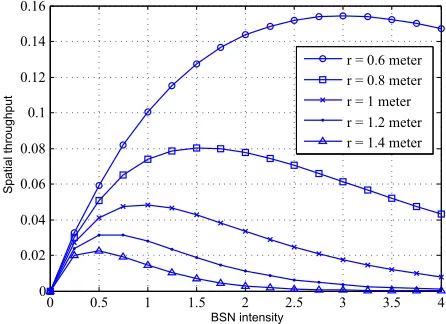
r = 0.6 meter r = 0.8 meter r = 1 meter r = 1.2 meter r = 1.4 meter

Fig. 10. Spatial throughput as a function of BSN intensity under different distancesrbetween sensor nodes in a BSN.w₁is set as 0.5 and interference detection range is 10 meter.

intensity, depending on which is more convenient, to achieve maximum spatial throughput.

F. Effects of the distances between sensor nodes in a BSN

Fig. 10 shows the spatial throughput as a function of BSN intensity under different distances between sensor nodes in a BSN. As can be seen, when the distance between sensor nodes in a BSN rincreases, the spatial throughput decreases for the same BSN intensity. This is because when r, i.e., the transmission distance, increases, the desired signal decreases. With the same interference, SINR decreases. Thus spatial throughput decreases as well.

V. CONCLUSION

throughput are derived in tractable expressions. Based on the analysis, two implications are given: 1) The interference detection range is optimized to achieve the maximum spatial throughput while the reliable transmission requirement is met. 2) The design of medium access control (MAC) for BSNs and the intensity of BSNs are optimized depending on the specific BSN applications.

Although the stochastic geometry analysis framework is designed for the inter-user interference in BSNs in this paper, it can also be applied to other networks where various MAC mechanisms are employed. For future work, we will evaluate the performance with extensive experiments.

ACKNOWLEDGMENT

This research was carried out at the SeSaMe Centre. It is supported by the Singapore NRF under its IRC@SG Funding Initiative and administered by the IDMPO.

REFERENCES

[1] G. Fortino, R. Giannantonio, R. Gravina, P. Kuryloski, and R. Jafari, “Enabling effective programming and flexible management of efficient body sensor ntwork applications,”IEEE Transaction on Human-Machine Systems, vol. 43, no. 1, pp. 115–133, 2013.

[2] J. Elias, S. Paris, and M. Krunz, “Cross technology interference mitigation in body area networks: an optimization approach,” IEEE Transaction on Vehicular Technology, 2014, early access.

[3] W. Sun, Y. Ge, and W. Wong, “A lightweight distributed scheme for mitigating inter-user interference in body sensor networks,”Computer Networks, vol. 57, no. 18, pp. 3885–3896, 2013.

[4] “IEEE standard for local and metropolitan area networks-Part 15.6: Wireless body area networks,”IEEE std 802.15.6-2012, pp. 1–271, 2012. [5] A. Natarajan, M. Motani, B. d. Silva, K. Yap, and K. Chua, “Investi-gating network architectures for body sensor networks,” inProc. ACM SIGMOBILE’07, San Juan, Puerto Rico, Jun. 2007.

[6] W. Sun, Y. Ge, and W. Wong, “Inter-user interference in body sensor networks: a case study in moderate-scale deployment in hospital envi-ronment,” inProc. IEEE HealthCom’12, Beijing, China, Oct. 2012. [7] P. Li and Y. Fang, “Impacts of topology and traffic pattern on capacity

of hybrid wireless networks,”IEEE Transaction on Mobile Computing, vol. 8, no. 12, pp. 1585–1595, 2009.

[8] X. Wang and L. Cai, “Interference analysis of co-existing wireless body area networks,” inProc. IEEE GLOBECOM’11, Houston, USA, Dec. 2011.

[9] H. EISawy, E. Hossain, and M. Haenggi, “Stochastic geometry for modeling, analysis, and design of multi-tier and cognitive cellular wire-less networks: a survey,”IEEE Communications Surveys and Tutorials, vol. 15, no. 3, pp. 996–1019, 2013.

[10] F. Baccelli, F. Blaszczyszyn, and P. Muhlethaler, “An aloha protocol for multihop mobile wireless networks,”IEEE Transaction on Information Theory, vol. 52, no. 2, pp. 421–436, 2006.

[11] H. Nguyen, F. Baccelli, and D. Kofman, “A stochastic geometry anal-ysis of dense IEEE 802.11 networks,” inProc. IEEE INFOCOM’07, Anchorage, USA, May 2007.

[12] Z. Tong, H. Lu, M. Haenggi, and C. Poellabauer, ”A Stochastic Geometry Approach to the Modeling of IEEE 802.11p for Vehicular Ad Hoc Networks”, 2013, Available at: http://www3.nd.edu/ mhaeng-gi/pubs/tvt14.pdf.

[13] A. Busson, G. Chelius, and J. Gorce, ”Interference modeling in CSMA multi-hop wireless networks”, INRIA, France, Tech. Rep. 6624, Feb. 2009.

[14] I. Kashiwagi, T. Taga, and T. Imai, “Time-varying path-shadowing model for indoor populated environments,” IEEE Transaction on Vehicular Technology, vol. 59, no. 1, pp. 16–28, 2010.

[15] A. Michalopoulou, A. Alexandridis, K. Peppas, T. Zervos, F. Lazarakis, K. Dangakis, and D. Kaklamani, “Statistical analysis for on-body spatial diversity communications at 2.45 GHz,”IEEE Transaction on Antennas and Propagation, vol. 60, no. 8, pp. 4014–4019, 2012.

[16] C. Kim, T. See, and T. Chiam, “Channel characterization of walking passerby effects on 2.48-GHz wireless body area network,” IEEE Transaction on Antennas and Propagations, vol. 61, no. 3, pp. 1495– 1498, 2013.

[17] J. Andrew, F. Baccelli, and R. Ganti, “A tratable approach to coverage and rate in cellular networks,”IEEE Transaction on Communications, vol. 59, no. 11, pp. 3122–3134, 2011.

[18] H. EISawy, E. Hossain, and M. Haenggi, “Spectrum-efficient multi-channel design for coexising IEEE 802.15.4 networks: a stochastic geometry approach,”IEEE Transactions on Mobile Computing, vol. 13, no. 7, pp. 1611–1624, 2014.

[19] Z. Gong and M. Haenggi, “Interference and outage in mobile random networks: expectation, distribution, and correlation,”IEEE Transaction on Mobile Computing, vol. 13, no. 2, pp. 337–349, 2012.

[20] K. Kwak, S. Ullah, and N. Ullah, “An overview of ieee 802.15.6 standard,” inProc. IEEE ISABEL’10, Rome, Italy, Jun. 2010. [21] B. Ramachandran and K. Lau, Funtional Equations in Probability

Theory. Elsevier, 2014.

[22] M. Haenggi, J. Andrew, F. Baccelli, O. Dousse, and M. Franceschitti, “Stochastic geometry and random graphs for the analysis and design of wireless networks,”IEEE Journal on Selected Areas in Communications, vol. 27, no. 7, pp. 1029–1045, 2009.

[23] P. Nardelli, ”Analysis of the spatial throughput in interference net-works”, Academic dissertation, University of Oulu, 2013, Available at: http://herkules.oulu.fi/isbn9789526201818/isbn9789526201818.pdf. [24] Scalable Network Technologies, Simulator, Qualnet Network, 2011,

Available at: http://www.qualnet.com.

[25] ”Wireless fundamentals: Signal-to-Noise Ratio (SNR) and wire-less signal strength”, Cisco Report, 2013, Available at: http-s://documentation.meraki.com/MR.

[26] T. Wang, W. Jia, G. Xing, and M. Li, “Exploiting statistical mobility models for efficient Wi-Fi deployment,”IEEE Transaction on Vehicular Technology, vol. 62, no. 1, pp. 360–373, 2013.

[27] H. Lee, M. Wicke, B. Kusy, O. Gnawali, and L. Guibas, “Predictive data delivery to mobile users through mobility learning in wireless sensor networks,” IEEE Transaction on Vehicular Technology, 2015, early access.

[28] N. Surobhi and A. Jamalipour, “M2M-based service coverage for mobile users in post-emergency enironments,”IEEE Transaction on Vehicular Technology, vol. 63, no. 7, pp. 3294–3303, 2014.

Wen Sunreceived the BEng degree in information technology from Harbin Institute of Technology, Harbin, China, in 2009, and the PhD degree in Department of Electrical and Computer Engineer-ing from National University of SEngineer-ingapore (NUS) in 2014. Since 2014, she has been working as a research fellow in Department of Computer Science, National University of Singapore. Her research in-terests include transmission schemes and resource management in wireless sensor networks.

Zhiqiang Zhangreceived the B.E. degree in com-puter science and technology from School of Elec-trical Information and Engineering, Tianjian Univer-sity, China, in 2005, and the Ph.D. degree from the Sensor Network and Application Research Center, Graduate University, Chinese Academy of Sciences, Beijing, China, in 2010. He is a research fellow in Department of Computing, Imperial College. His research interests include Body Sensor Network, Information Fusion and Targets Tracking.